Estimating trajectories of meteors: an observational Monte Carlo approach - II. Results - UWO Physics & Astronomy
←
→
Page content transcription
If your browser does not render page correctly, please read the page content below
MNRAS 491, 3996–4011 (2020)                                                                                                doi:10.1093/mnras/stz3338
Advance Access publication 2019 November 28

Estimating trajectories of meteors: an observational Monte Carlo
approach – II. Results

Denis Vida ,1,2‹ Peter G. Brown,2,3‹ Margaret Campbell-Brown ,2,3 Paul Wiegert2,3

                                                                                                                                                         Downloaded from https://academic.oup.com/mnras/article-abstract/491/3/3996/5645268 by University of Western Ontario user on 09 January 2020
and Peter S. Gural4‹
1 Department  of Earth Sciences, University of Western Ontario, London, Ontario N6A 5B7, Canada
2 Department  of Physics and Astronomy, University of Western Ontario, London, Ontario N6A 3K7, Canada
3 Centre for Planetary Science and Exploration, University of Western Ontario, London, Ontario N6A 5B8, Canada
4 Gural Software and Analysis LLC, Sterling, Virginia, 20164, USA

Accepted 2019 November 25. Received 2019 November 10; in original form 2019 September 23

                                       ABSTRACT
                                       In the first paper of this series, we examined existing methods of optical meteor trajectory
                                       estimation and developed a novel method which simultaneously uses both the geometry and
                                       the dynamics of meteors to constrain their trajectories. We also developed a simulator which
                                       uses an ablation model to generate realistic synthetic meteor trajectories which we use to test
                                       meteor trajectory solvers. In this second paper, we perform simulation validation to estimate
                                       radiant and velocity accuracy, which may be achieved by various meteor observation systems
                                       as applied to several meteor showers. For low-resolution all-sky systems, where the meteor
                                       deceleration is generally not measurable, the multi-parameter fit method assuming a constant
                                       velocity better reproduces the radiant and speed of synthetic meteors. For moderate field of
                                       view systems, our novel method performs the best at all convergence angles, while multi-
                                       parameter fit methods generally produce larger speed errors. For high-resolution, narrow field
                                       of view systems, we find our new method of trajectory estimation reproduces radiant and
                                       speed more accurately than all other methods tested. The ablation properties of meteoroids
                                       are commonly found to be the limiting factor in velocity accuracy. We show that the true
                                       radiant dispersion of meteor showers can be reliably measured with moderate field of view
                                       (or more precise) systems provided appropriate methods of meteor trajectory estimation are
                                       employed. Finally, we compare estimated and real angular radiant uncertainty and show that
                                       for the solvers tested the real radiant error is on average underestimated by a factor of two.
                                       Key words: comets: general – meteors – meteoroids.

                                                                              the earliest measured luminous point of the meteor, a topic addressed
1 I N T RO D U C T I O N
                                                                              in Vida et al. (2018).
This paper is a direct continuation of an earlier work (Vida et al.              In Paper 1, we analyzed the shortcomings of existing methods of
2019b, hereafter Paper 1), in which we developed both a new                   meteor trajectory estimation, with particular focus on application
method for estimating meteor trajectories and a meteor trajectory             to the high-precision data collected by the Canadian Automated
simulator. Paper 1 also presented a summary of the theory behind              Meteor Observatory’s (CAMO) mirror tracking system (Weryk et al.
earlier meteor trajectory determination algorithms. In this paper             2013). In Paper 1, we examined the most commonly used meteor
we attempt to answer the following question: For a given type of              trajectory estimation methods in detail, including: the geometrical
optical meteor observation system, what is the best trajectory solver         intersecting planes (Ceplecha 1987) and lines of sight (Borovička
to use, and what is the associated expected quantitative accuracy?            1990) approaches, and the multi-parameter fit (MPF) method by
We note that this is only the first step in the process of estimating         Gural (2012). As pointed out by Egal et al. (2017), the true mea-
a meteoroid’s original heliocentric orbit. The necessary additional           surement accuracy of these methods for various meteor observation
step is accounting for deceleration due to atmospheric drag prior to          systems and showers is unknown, and the most advanced of them,
                                                                              the MPF method with the exponential deceleration velocity model,
                                                                              is numerically problematic to fit to observations.
E-mail: dvida@uwo.ca (DV); pbrown@uwo.ca (PGB); pgural@gmail.                   In an attempt to improve on existing algorithms, we developed
com (PSG)                                                                     a novel meteor trajectory estimation method which uses both the

                                                                                                                                 C 2019 The Author(s)

                                                                      Published by Oxford University Press on behalf of the Royal Astronomical Society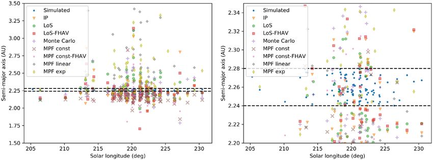
Novel meteor trajectory solver                  3997
geometry and the dynamics of a meteor to constrain a trajectory              (iii) An image intensified mirror tracking system based on the
solution, but without an assumed underlying kinematic model. We            Canadian Automated Meteor Observatory (CAMO) (Weryk et al.
also developed a meteor trajectory simulator which uses the meteor         2013).
ablation model of Campbell-Brown & Koschny (2004) to simulate
                                                                           These systems cover a wide range of observed meteoroid masses,
realistic dynamics and light curves of meteors given their physical
                                                                           fields of view, and astrometric precision. Details of each system are
properties as a means to compare and test meteor trajectory solvers.
                                                                           given in Table 1.
   In this work, we apply the simulator and explore the accuracy
                                                                              Our simulated all-sky fireball network consisted of 3 stations in an

                                                                                                                                                     Downloaded from https://academic.oup.com/mnras/article-abstract/491/3/3996/5645268 by University of Western Ontario user on 09 January 2020
of each trajectory solver to three types of typical optical meteor
                                                                           equilateral triangle configuration with 100 km long sides (stations
observation systems: a low-resolution all-sky system, a moderate
                                                                           A1, A2, and A3 in the simulation). The cameras at each station
field of view system, and the high-precision CAMO mirror tracking
                                                                           are pointing straight up and have a field of view (FOV) of 120◦ ×
system. For each system we used the simulator to investigate the
                                                                           120◦ . Larger FOVs were difficult to simulate as the volume of the
ability of each solver to properly recover the geocentric radiant and
                                                                           sky that needed to be randomly sampled becomes very high, and
velocity of three major showers spanning a wide range of meteor
                                                                           most of it was outside the FOV of other cameras. The measurement
velocities and meteoroid types (Draconids, Geminids, Perseids).
                                                                           uncertainly was assumed to be 2 arc minutes and the frames per
The parameters used for simulations and the comparison between
                                                                           second (FPS) of the cameras 30.
simulations and real-world observations are given in Section 2. We
                                                                              For the CAMS-like moderate FOV system, we also chose to use
also perform dynamical modelling of the 2011 Draconid outburst,
                                                                           3 stations in the equilateral triangle configuration (stations M1, M2,
which was produced by recently ejected meteoroids (Vaubaillon
                                                                           and M3 in the simulation). These had FOVs of 64◦ × 48◦ , 30 FPS
et al. 2011) and thus should have a very tight radiant. We use
                                                                           and a measurement uncertainly of 30 arc seconds. The elevation of
this compact shower to estimate the radiant measurement accuracy
                                                                           the centres of the fields of view of all cameras was 65◦ and they
needed to resolve the true physical dispersion of a meteor shower.
                                                                           where all pointed towards the centre of the triangle.
   In Section 3, we present simulation results and compare the
                                                                              Finally, the simulated CAMO system mimics the real system
performance of various meteor trajectory estimation methods across
                                                                           which has 2 stations (‘tavis’ and ‘elgin’ in the simulation) separated
all simulated meteor observation systems and our three chosen
                                                                           by 45 km, a FOV of 30◦ × 30◦ , cameras operated at 100 FPS, and
showers. In Section 3.5, we examine solver performances as applied
                                                                           a precision of 1 arc second.
to a specific case study, namely the unique 2015 Taurid outburst.
This outburst was arguably the first instance where we have both
strong a priori knowledge of the expected orbits (particularly             2.2 Simulated meteor showers
semi-major axis) and a large number of high – precision meteor
trajectories (Spurnỳ et al. 2017). We also consider the special case of   To explore the performance of various meteor trajectory estimation
long duration fireballs where the influence of gravity is particularly     methods when observing meteors of different velocities and phys-
important by simulating solver performance for an all-sky system as        ical properties we focused on generating synthetic meteors from
will be discussed in Section 3.6. Finally, in Section 3.7 we examine       three very different meteor showers. We simulated 100 meteors for
the accuracy of meteor trajectory error estimation by comparing            every system for each of the following three meteor showers:
estimated radiant errors to offsets from the simulated ground                 (i) The 2011 Draconids, a low-velocity (∼ 21 km s−1 ) shower
truth.                                                                     with fragile and fresh (2000 yr ago
solvers with the new Monte Carlo method, we appeal to simula-              (Brown & Jones 1998).
tions. The method of generating simulated meteor observations is
                                                                           Realistic trajectories and dynamics were simulated using the
described in detail in Paper 1 (Vida et al. 2019b). We simulated three
                                                                           Campbell-Brown & Koschny (2004) meteoroid ablation model
optical meteor observation systems to generate synthetic meteors
                                                                           procedure described in detail in Vida et al. (2018). Meteor shower
to feed into each trajectory simulator. These three systems follow
                                                                           parameters used in the simulations are given in Table 2 – parameters
the optical model system choices previously discussed in Vida et al.
                                                                           of all showers except the Draconids were taken from observations
(2018). The characteristics of these systems (which largely vary in
                                                                           published in the literature.
terms of angular precision) include:
                                                                              Note that the 2015 Taurid fireball outburst was also simulated, but
   (i) A low resolution all-sky CCD video fireball system based on         only for the all-sky systems as discussed in Section 3.5. The goal
the hardware of the Southern Ontario Meteor Network (SOMN)                 in applying our analysis to the unique 2015 Taurid outburst was
(Brown et al. 2010).                                                       to contrast the accuracy of various trajectory estimation methods
   (ii) A moderate field of view CCD video system typical of CAMS          when using low-precision (video) all-sky systems as compared to
(Jenniskens et al. 2011), SonotaCo,1 the Croatian Meteor Network           higher precision fireball systems.
(Gural & Šegon 2009), and the Global Meteor Network (Vida et al.
2019a).
                                                                           2.3 Dynamical modelling of the 2011 Draconid outburst
                                                                           The 2011 Draconids were the youngest of the simulated showers
1 SonotaCo:   http://sonotaco.jp/                                          and should have the most compact radiant. The measured radiant

                                                                                                              MNRAS 491, 3996–4011 (2020)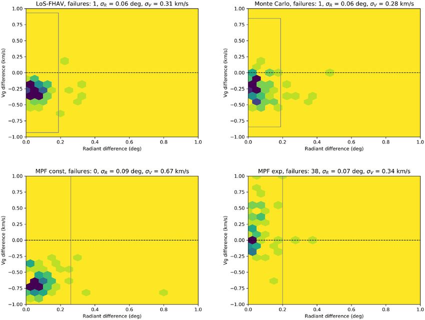
3998        D. Vida et al.
            Table 1. Parameters of simulated optical meteor observation systems. tmax is the maximum time offset, FPS is the FPS of the
            camera, σ obs the measurement uncertainly in arc seconds, FOV width and height are the size of the field of view in degrees, MLM
            the meteor limiting magnitude, and P0m is the power of a zero-magnitude meteor (power values taken from Weryk & Brown 2013).

            System         N stations      tmax (s)     FPS        σ obs (arcsec)      FOV width (deg)       FOV height (deg)       MLM     P0m (W)

            CAMO               2               1         100             1                      30                     30            +5.5       840
            Moderate           3               1          30             30                     64                     48            +5.0      1210

                                                                                                                                                                       Downloaded from https://academic.oup.com/mnras/article-abstract/491/3/3996/5645268 by University of Western Ontario user on 09 January 2020
            All-sky            3               1          30            120                     120                    120           − 0.5     1210

      Table 2. The model parameters adopted for simulated meteor showers. The parameters for the Draconids were computed from the simulation as
      discussed in the text. The parameters for the Geminids and Perseids were taken from Jenniskens et al. (2016) unless otherwise noted. Parameters
      for the 2015 Taurids were taken from Spurnỳ et al. (2017). These were modified from the original so that they are centered around the peak solar
      longitude while the radiant spread was computed directly from data provided in Spurnỳ et al. (2017). λmax      is the solar longitude of the peak
      (degrees), B is the solar longitude slope of the rising portion of the activity profile following the procedure of Jenniskens (1994), α is the mean
      geocentric right ascension, α is the radiant drift (degree on the sky per degree of solar longitude), α σ is the standard deviation in R.A., δ is the
      mean geocentric declination, δ is the declination radiant drift, δ σ is the standard deviation of the declination, Vg is the mean geocentric velocity
      in km s−1 , Vg is the change in geocentric velocity per degree of solar longitude, and Vgσ is the standard deviation of the geocentric velocity.

      Shower                        Year     λmax
                                                          B           α         α        ασ          δ       δ            δσ      Vg       Vg      Vgσ

      Draconids                     2011    198.07     17.5,   1∗   263.39      0.0       0.29        55.92     0.0          0.16   20.93      0       0.04
      Geminids                      2012    262.0      ∼0.5, 2∗     113.5       1.15      2.8         32.3    − 0.16         1.5    33.8       0       2.0
      Perseids                      2012    140.0       0.4, 2∗      48.2       1.4       2.8         58.1      0.26         1.7    59.1       0       2.4
      Taurids – resonant branch     2015    221.0       0.15         53.06      0.554     0.33        14.66     0.06         0.27   29.69    −0.293    0.22
      Note.1∗ – (Koten et al. 2014), 2∗ – (Jenniskens 1994)

spread should be dominated by measurement uncertainty when
measured with less precise systems. To quantify the minimum
accuracy required to observe the true physical radiant and velocity
dispersion of the 2011 Draconids, we appeal to dynamical modelling
of the shower. Here we use the method of Wiegert et al. (2009) to
obtain an estimate of both the true average location of the radiant
and velocity of the outburst and its theoretical spread. We then
use these as inputs to our simulation model to generate synthetic
2011 Draconids to virtually ‘observe’ with each of our three optical
systems and apply each meteor trajectory solver in turn.
   To dynamically model the 2011 Draconid outburst, the orbital
elements of the 1966 apparition of 21P/Giacobini-Zinner were
integrated backwards 200 years with the RADAU (Everhart 1985)
integrator within a simulated Solar System containing the Sun and
eight planets. The parent comet was then advanced forward in time
while ejecting meteoroids with radii between 100 μm and 10 cm
when within 3 AU of the Sun. The ejection speed and direction                         Figure 1. Density map of simulated geocentric equatorial (J2000.0) radi-
follows the approach of the Brown & Jones (1998) model with an                        ants of the 2011 Draconids at the time of peak activity. A bi-variate Gaussian
assumed comet radius of 1 km, albedo of 0.05 and bulk density of                      was fit to the radiants (α g = 263.387◦ ± 0.291◦ , δ g = 55.9181◦ ± 0.158◦ ).
300 kg m−3 .                                                                          The corresponding 2σ level is shown as a black contour. Draconid radiants
   Meteoroids arriving at Earth in 2011 were found to be produced                     observed by Borovička et al. (2014) in 2011 are also shown.
by the 1838 and 1907 comet perihelion passages, with smaller
contributions from 1920 and 1953. The simulated peak coincided                        radiants. Distinct radiant structure can also be seen – we estimate
with that reported by visual observers2 to the International Me-                      that an observational radiant precision of better than 3 to 6 arc
teor Organization (IMO) Visual Meteor Database (Roggemans                             minutes (0.05◦ – 0.1◦ ) is needed for the true radiant structure to
1988).                                                                                be unambiguously reconstructed from observations. We use these
   The radiants of the dynamically modelled stream that impacted                      values as the absolute minimum radiant accuracy needed to resolve
the Earth are shown in Fig. 1. Note that these model radiants are                     the true physical radiant spread for showers with the most compact
without observational biases because they were directly computed                      radiants.
from simulated meteoroids arriving at Earth. The position and the                        The video and high power large aperture (HPLA) observations
dispersion of the modelled radiant at the time of peak activity                       of the Draconid outburst measured an almost order of magnitude
was α g = 263.387◦ ± 0.291◦ , δ g = 55.9181◦ ± 0.158◦ . The                           larger dispersion than our model predicts, suggesting they did not
values were derived by fitting a bi-variate Gaussian to the modelled                  record the intrinsic (physical) radiant spread of the shower (Kero
                                                                                      et al. 2012; Trigo-Rodrı́guez et al. 2013; Šegon et al. 2014). We
2 IMO VMDB 2011 Draconids: https://www.imo.net/members/imo
                                                                                      note that the video observations of the outburst incorporating high-
                                                                     live sho
                                                                                      quality manual reductions reported by Borovička et al. (2014) are
wer?shower=DRA&year = 2011

MNRAS 491, 3996–4011 (2020)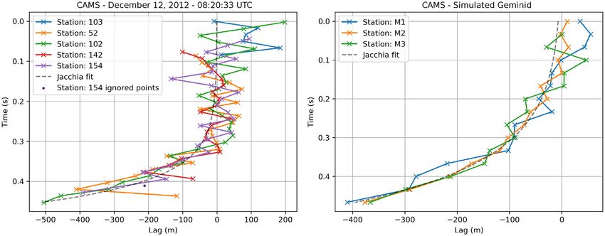
Novel meteor trajectory solver                  3999
Table 3. Physical properties of meteoroids adopted as input to the ablation      properties of shower meteoroids used in the ablation modeling in
model in simulating our four meteor showers. Here s is the mass index,           Table 3.
ρ is the range of bulk densities of meteoroids, σ is the apparent ablation
coefficient (Ceplecha & ReVelle 2005), and L is the energy needed to ablate
a unit of meteoroid mass.                                                        2.4 Simulation validation
                                                                                 To confirm the appropriateness of the simulations, we compare
Shower          s         ρ (kg m−3 )            σ (s2 km−2 )      L (J kg−1 )
                                                                                 some metrics among our suite of simulated and observed meteors
            1.95, 1∗   100–400, 2∗             0.21, D-type, 3∗    1.2 × 10⁶

                                                                                                                                                           Downloaded from https://academic.oup.com/mnras/article-abstract/491/3/3996/5645268 by University of Western Ontario user on 09 January 2020
Draconids                                                                        for the same optical system. Note that we did not attempt to
Geminids    1.7, 4∗   1000–3000, 5∗            0.042, A-type, 3∗   6.0 × 106     reconstruct particular observed events though simulation; we only
Perseids    2.0, 7∗ HTC distribution, 6∗       0.1, C-type, 3∗     2.5 × 10⁶     identified meteors of similar properties and quantitatively compared
Taurids     1.8, 8∗   1200–1600, 9∗            0.1, C-type, 3∗     2.5 × 10⁶
                                                                                 the trajectory fit residuals and deceleration. As an indicator of
Note.1∗ – (Koten et al. 2014), 2∗ – (Borovička et al. 2007), 3∗ – (Ceplecha     deceleration we computed the meteor’s lag, i.e. how much the
et al. 1998), 4∗ – (Blaauw, Campbell-Brown & Weryk 2011), 5∗ – (Borovička       observed meteor falls behind a hypothetical meteoroid moving with
et al. 2009), 6∗ – (Moorhead et al. 2017), 7∗ – (Beech & Nikolova 1999), 8∗      a fixed speed equal to the initial velocity. We present several meteors
– (Moser et al. 2011), 9∗ – (Brown et al. 2013)
                                                                                 from instrument data sets having comparable speed and duration
                                                                                 to those we simulated. Table 4 compares the initial speed, mass
Table 4. Comparison of several selected observed meteors and the close           and zenith angle of a selection of simulated and representative
fits from among the simulated set of meteors. The photometric masses were        observed meteors. All observations were reduced using the Monte
computed using a dimensionless luminous efficiency of τ = 0.7 per cent           Carlo method.
(Vida et al. 2018) and a bandpass specific P0m = 1210 W. The observed               As a first example, Figs 2 and 3 show a sporadic meteor with
(calculated) masses are similar to simulated masses. Note that the range of      a geocentric velocity Vg =∼ 21 km s−1 observed with CAMO and
simulated masses was taken from Vida et al. (2018) and is based on the
                                                                                 comparable simulated CAMO Draconid. The ‘Jacchia fit’ curve
masses calculated from observations by each type of system.
                                                                                 in lag plots is a fit of the exponential deceleration model of
System        Initial speed (km/s)       Mass (g)       Zenith angle (deg)
                                                                                 Whipple & Jacchia (1957) to the computed lag and is only used
               Obs           Sim        Obs    Sim         Obs         Sim       for visualization purposes. The amount of deceleration and the
                                                                                 scatter in the spatial fit residuals (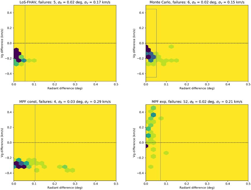
4000        D. Vida et al.

                                                                                                                                                           Downloaded from https://academic.oup.com/mnras/article-abstract/491/3/3996/5645268 by University of Western Ontario user on 09 January 2020
Figure 3. Left: Spatial residuals of a CAMO sporadic meteor observed on October 7, 2016 with Vg = 21.4 km s−1 . Station 1 is Tavistock, 2 is Elginfield.
Right: A simulated CAMO Draconid of similar mass and with Vg = 20.9 km s−1 .

Figure 4. Left: Lag of a CAMS Geminid observed on December 12, 2012 with Vg = 33.4 km s−1 by CAMS cameras in California. Right: A simulated
CAMS Geminid of similar mass with Vg = 34.6 km s−1 .

   Finally, Fig. 5 shows the comparison for a low-resolution, all-             of the trajectory; better initial velocity accuracy might be achieved
sky system, namely the Southern Ontario Meteor Network Brown                   by using the method of Pecina & Ceplecha (1983, 1984).
et al. (2010) between an observed Southern Taurid (Vg = 31.4                      (ii) LoS – Our implementation of the Borovička (1990) method
km s−1 ) and a simulated Geminid. Neither meteor shows visible                 with our progressive initial velocity estimation method as described
deceleration due to the low precision of the measurements. However,            in Paper 1.
deceleration may become visible and significant for much longer                   (iii) LoS-FHAV – Our implementation of the Borovička (1990)
duration fireballs (see Section 3.6).                                          method. The initial velocity is computed as the average velocity of
                                                                               the first half of the trajectory.
                                                                                  (iv) MC – The Monte Carlo method presented in Paper 1.
3 R E S U LT S                                                                    (v) MPF const – The multi-parameter fit method of Gural (2012)
Following the theoretical development given in Paper 1, we numer-              using a constant velocity model.
ically evaluated the performance of the following trajectory solvers              (vi) MPF const-FHAV – For this hybrid-solver, the radiant
(abbreviations used later in the text):                                        solution is taken from the MPF constant velocity model, but the lines
                                                                               of sight are re-projected on the trajectory and the initial velocity is
   (i) IP – The intersecting planes method of Ceplecha (1987). The             estimated as the slope of the length versus time along the track
initial velocity is computed as the average velocity of the first half         (effectively, the average velocity) of the first half of the trajectory.

MNRAS 491, 3996–4011 (2020)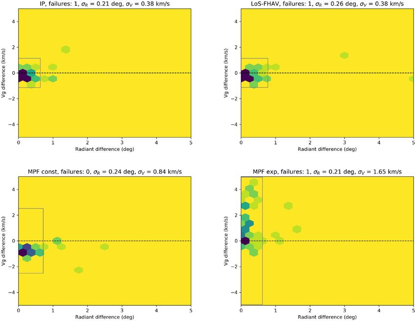
Novel meteor trajectory solver               4001

                                                                                                                                                           Downloaded from https://academic.oup.com/mnras/article-abstract/491/3/3996/5645268 by University of Western Ontario user on 09 January 2020
Figure 5. Left: Lag of a SOMN Southern Taurid meteor observed on October 10, 2018 with Vg = 31.4 km s−1 . Ignored points are those with angular error
more than 3σ above the mean after the first trajectory estimation pass as described in Paper 1. Right: A simulated SOMN Geminid with Vg = 34.0 km s−1 .

                  Table 5. Comparison of solver accuracy for a simulated three station all-sky system. The trajectory was taken to be
                  valid for simulation if the converge angle was larger than 15◦ . F is the number of failures (out of 100), i.e. the number
                  of radiants that were outside the window bounded by Rmax = 5◦ , V max = 5 km s−1 .

                  Solver                               DRA                                GEM                               PER
                                        F       σR             σV          F       σR             σV           F       σR             σV

                  IP                    1      0.44◦      0.38 km s−1      1      0.21◦      0.38 km s−1      10     0.67◦        0.99 km s−1
                  LoS                   1      0.56◦      0.47 km s−1      1      0.26◦      0.42 km s−1       3     0.66◦        0.46 km s−1
                  LoS-FHAV              1      0.51◦      0.38 km s−1      1      0.26◦      0.38 km s−1       7     0.66◦        0.53 km s−1
                  Monte Carlo           2      0.52◦      0.36 km s−1      1      0.24◦      0.47 km s−1       4     0.80◦        0.38 km s−1
                  MPF const             1      0.28◦      0.46 km s−1      0      0.24◦      0.84 km s−1       1     0.47◦        0.37 km s−1
                  MPF const-FHAV        1      0.27◦      0.38 km s−1      0      0.23◦      0.41 km s−1       4     0.35◦        0.80 km s−1
                  MPF linear            0      0.26◦      0.54 km s−1      4      0.23◦      1.76 km s−1       6     0.35◦        0.60 km s−1
                  MPF exp               0      0.41◦      1.39 km s−1      1      0.21◦      1.65 km s−1      12     0.32◦        1.18 km s−1

  (vii) MPF linear – The Gural (2012) multi-parameter fit method                     A trajectory solution was considered to be a failure if the radiant
with a linear deceleration velocity model.                                        error (difference between estimated and true as initially input into
  (viii) MPF exp – The Gural (2012) multi-parameter fit method                    the simulation) was more than Rmax degrees from the true radiant,
with the exponential deceleration model of Whipple & Jacchia                      or if the velocity error was more than Vmax from the model velocity.
(1957)                                                                            For the simulated all-sky system the values used were Rmax =
                                                                                  5◦ , V max = 5 km s−1 , while for the moderate FOV (CAMS-like)
   Global results for all tested trajectory solvers for all-sky systems
                                                                                  system we adopted Rmax = 1◦ , V max = 1 km s−1 . Finally, for the
are given in Table 5, for moderate FOV systems in Table 6, and
                                                                                  simulated CAMO–like system, we adopted Rmax = 0.5◦ , V max =
for CAMO in Table 7, respectively. For every combination of
                                                                                  0.5 km s−1 .
observation system, meteor shower and trajectory solver we list:
                                                                                     Solutions were also removed from further consideration if any of
                                                                                  the multi-station convergence angles were less than 15◦ , 10◦ , and 1◦
   (i) The column labelled F in each table is the total number                    for the all-sky, CAMS, and CAMO simulations respectively. This
of failures for a given method out of 100 simulated runs. This                    procedure was adopted so that the general performance of different
is the number of trajectory solutions with radiant or velocity                    solvers can be compared, excluding excessive deviations due simply
difference between the true (simulated) and estimated values                      to low convergence angles. We explore in more depth the depen-
larger than the predetermined values given in the caption to each                 dence of solution accuracy on the convergence angle in Section 3.4.
table.                                                                               In what follows, we show representative plots of the spread in
   (ii) The standard deviation between the estimated and true radiant             the radiant and velocity accuracy for each trajectory solver for each
angular separation (σ R in tables).                                               optical system. In addition, we show a selection of individual results
   (iii) The standard deviation between the estimated and true                    per shower and per solver in the form of 2D histograms (e.g. Fig. 7)
geocentric velocity (σ V in tables).                                              which highlight the scatter of estimates among the 100 simulated
The standard deviations are computed after iteratively rejecting                  meteors. On these plots, the angular distance between the real and
solutions outside 3σ .                                                            the estimated geocentric radiant is shown on the X axis, the error in

                                                                                                                         MNRAS 491, 3996–4011 (2020)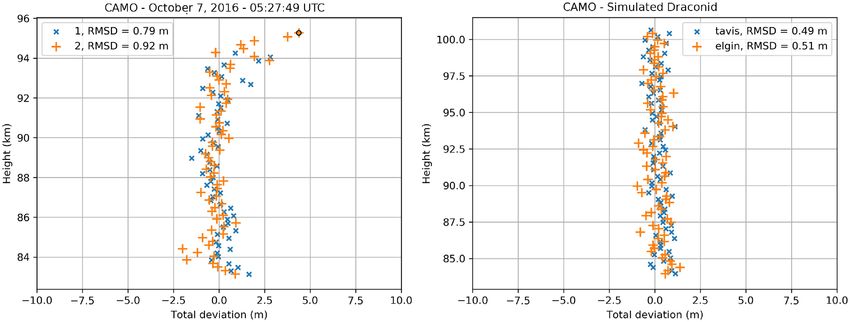
4002        D. Vida et al.
                  Table 6. Solver performance comparison for the simulated moderate FOV system. The trajectory was included in the
                  statistics if the convergence angle was larger than 10◦ . F is the number of failures (out of 100), i.e. the number of
                  radiants that were outside the Rmax = 1◦ , V max = 1 km s−1 window.

                  Solver                                DRA                                 GEM                               PER
                                         F       σR             σV           F       σR             σV           F       σR             σV

                  IP                    1       0.07◦      0.15 km s−1       1      0.06◦      0.31 km s−1       5      0.07◦       0.17 km s−1
                                                0.09◦      0.17 km s−1              0.06◦      0.29 km s−1              0.07◦       0.16 km s−1

                                                                                                                                                                   Downloaded from https://academic.oup.com/mnras/article-abstract/491/3/3996/5645268 by University of Western Ontario user on 09 January 2020
                  LoS                   1                                    1                                   2
                  LoS-FHAV              1       0.09◦      0.13 km s−1       1      0.06◦      0.31 km s−1       5      0.08◦       0.17 km s−1
                  Monte Carlo           2       0.08◦      0.15 km s−1       1      0.06◦      0.28 km s−1       2      0.09◦       0.15 km s−1
                  MPF const             1       0.08◦      0.26 km s−1       0      0.09◦      0.67 km s−1       0      0.06◦       0.22 km s−1
                  MPF const-FHAV        9       0.08◦      0.35 km s−1       6      0.08◦      0.37 km s−1       8      0.06◦       0.32 km s−1
                  MPF linear            19      0.07◦      0.39 km s−1      34      0.07◦      0.45 km s−1       6      0.05◦       0.19 km s−1
                  MPF exp               34      0.07◦      0.50 km s−1      38      0.07◦      0.34 km s−1       9      0.06◦       0.37 km s−1

                  Table 7. Solver performance comparison for the simulated CAMO-like optical system. A simulated trajectory was
                  included in the final statistics if the convergence angle was larger than 1◦ . F is the number of failures (out of 100), i.e.
                  the number of radiants that were outside the Rmax = 0.5◦ , V max = 0.5 km s−1 window.

                  Solver                                DRA                                 GEM                               PER
                                         F       σR             σV           F       σR             σV           F       σR             σV

                  IP                    5       0.02◦      0.18 km s−1      24      0.01◦      0.33 km s−1       1      0.01◦       0.14 km s−1
                  LoS                   8       0.02◦      0.15 km s−1      17      0.01◦      0.27 km s−1       1      0.01◦       0.12 km s−1
                  LoS-FHAV              5       0.02◦      0.17 km s−1      23      0.02◦      0.33 km s−1       1      0.01◦       0.14 km s−1
                  Monte Carlo           6       0.02◦      0.15 km s−1      18      0.01◦      0.27 km s−1       1      0.01◦       0.11 km s−1
                  MPF const             4       0.03◦      0.29 km s−1      99      0.31◦      0.47 km s−1       5      0.03◦       0.23 km s−1
                  MPF const-FHAV        12      0.03◦      0.18 km s−1      43      0.17◦      0.35 km s−1      28      0.03◦       0.26 km s−1
                  MPF linear            43      0.02◦      0.22 km s−1      62      0.03◦      0.33 km s−1      22      0.01◦       0.19 km s−1
                  MPF exp               52      0.02◦      0.21 km s−1      68      0.02◦      0.27 km s−1      56      0.01◦       0.26 km s−1

the geocentric velocity is shown on the Y axis, and the bin count is
colour coded (darker colour means higher count).

3.1 All-sky systems
Table 5 lists the accuracy of geocentric radiants computed for the
simulated showers using different methods of meteor trajectory
estimation for a three station all-sky system. Fig. 6 is a visualization
of the values in the table. The numbers above the vertical bars for
each solver represent the failure rate (out of 100) for the Draconids,
the Geminids and the Perseids (in that order). Fig. 7 shows the
distribution of radiant and velocity errors as 2D hexbin histograms
for a selection of solvers applied to simulated Geminid data. The
increasing bin count is colour coded with increasingly darker colors.
The grey boxes show the 3σ standard deviation.
   From Fig. 6 it is apparent that the IP and LoS methods achieve
decent radiant accuracy, but tend to have a larger number of
failures for faster meteors (Perseids). Moreover, the estimated                     Figure 6. Comparison of geocentric radiant and velocity accuracy for a
                                                                                    simulated three station all-sky system for three simulated showers and the
velocity accuracy decreases with meteor speed, a direct con-
                                                                                    various trajectory solvers. The numbers at the top of each vertical bar show
sequence of the smaller number of data points on which the                          the number of failures for a particular method (given in red text) for the
velocity can be estimated for these methods. The Monte Carlo                        Draconids, Geminids and Perseids simulated, respectively.
method does not provide any significant increase in accuracy as
expected, as the limited precision does not produce useful lag                      all-sky data, simultaneously achieving good radiant accuracy and
measurements.                                                                       a low number of failures, even for faster meteors. Note, however,
   Fig. 7 shows that the MPF exponential velocity model tends to                    that because the MPF constant velocity model only computes the
overestimate velocities at infinity (a behaviour of the exponential                 average velocity, the velocity estimation is precise but not accurate;
deceleration function also noticed by Pecina & Ceplecha 1983)                       it is systematically underestimated. The use of the MPF const-
and that it has a noticeably larger number of failures for faster                   FHAV was an attempt to improve on this deficiency by computing
meteoroids than other methods (except the IP). In contrast, the MPF                 the initial velocity as equal to the average velocity of the first half of
constant velocity model is the most robust all-around solver for                    the trajectory. This works well for the Draconids and the Geminids,

MNRAS 491, 3996–4011 (2020)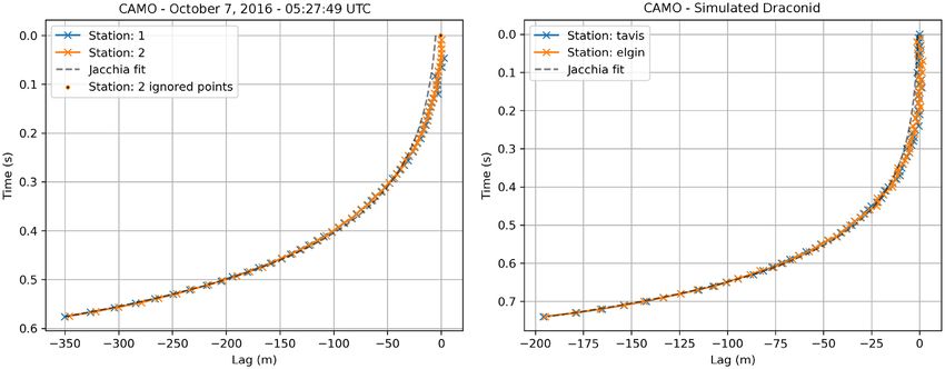
Novel meteor trajectory solver                         4003

                                                                                                                                                                          Downloaded from https://academic.oup.com/mnras/article-abstract/491/3/3996/5645268 by University of Western Ontario user on 09 January 2020
Figure 7. Accuracy of geocentric radiants for the Geminids simulated for all-sky systems shown as a density plot (darker is denser). Upper left: Intersecting
planes. Upper right: Lines of sight, initial velocity estimated as the average velocity of the first half of the trajectory. Bottom left: Multi-parameter fit, constant
velocity model. Bottom right: Multi-parameter fit, exponential velocity model.

but produces a significantly higher error for the faster Perseids,
where the reduction in number of measured points leads to a much
larger error.
   From our simulations, it appears that the optimal operational
approach for low resolution (video) all-sky systems would be to
adopt the MPF solver with the constant velocity model, plus a
separate (empirical) deceleration correction. The expected geo-
centric radiant error with this solver is around 0.25◦ (0.5◦ for
the Perseids) and around 500 m s−1 in velocity (or 250 m s−1 if
additional compensation for the early, pre-luminous deceleration is
included).

3.2 Moderate FOV systems
Table 6 lists the accuracy of geocentric radiants computed for
individual showers using different methods of meteor trajectory
estimation for simulated meteors detected by a three station CAMS-
type optical system. Fig. 8 shows the visualization of the values in                   Figure 8. Comparison of the geocentric radiant and velocity accuracy for
the table.                                                                             a simulated CAMS-type system for three showers and various trajectory
   The situation is more complex than was the case for the all-                        solvers.
sky system. For convergence angles >10◦ , the best results are
produced by the classical intersecting planes and the lines of sight

                                                                                                                               MNRAS 491, 3996–4011 (2020)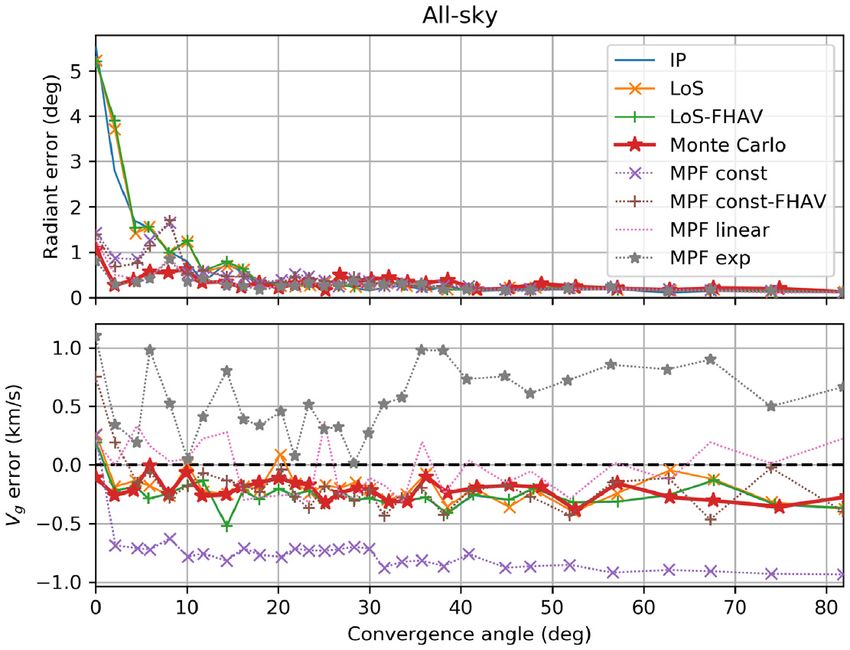
4004        D. Vida et al.

                                                                                                                                                               Downloaded from https://academic.oup.com/mnras/article-abstract/491/3/3996/5645268 by University of Western Ontario user on 09 January 2020
Figure 9. Accuracy of geocentric radiants for the Geminids simulated for CAMS-like systems. Upper left: Lines of sight, initial velocity estimated as
the average velocity of the first half of the trajectory. Upper right: Monte Carlo. Bottom left: Multi-parameter fit, constant velocity model. Bottom right:
Multi-parameter fit, exponential velocity model.

solvers, while the solvers which include kinematics perform either               high failure rate for this type of data as well, predominantly due
marginally worse in the case of the Monte Carlo solver, or sig-                  to the overestimation of the initial velocity. On the other hand, the
nificantly worse in the case of multi-parameter fit methods. For all             radiant estimation was as robust as the other solvers, for events
solvers, events which led to a solution within our acceptance window             which met our acceptance criteria. This finding is worrisome as
correspond to expected radiant errors around 0.1◦ . The velocity error           this velocity model was used by the CAMS network (Jenniskens
is around 200 m s−1 (around 100 m s−1 after deceleration correction)             et al. 2016). Our simulations suggest that initial velocities obtained
for the better solvers. The exception are the Geminids which have                with MPF-exp for moderate field of view systems should ideally be
a factor of 2 larger velocity uncertainties. They penetrate deeper               compared to other solvers before acceptance.
into the atmosphere due to their asteroidal composition, and decel-
erate more, which leads to a larger underestimation of the initial
velocity.                                                                        3.3 CAMO system
   We emphasize that the MPF methods sometimes do produce
better estimates of the radiant, which is consistent with Gural                  Table 7 lists the accuracy of geocentric radiants for our three
(2012) who only investigated the precision of the radiant position for           modelled showers using different methods of meteor trajectory
various solvers. On the other hand, MPF-based velocity estimates                 estimation applied to simulated CAMO data. Fig. 10 shows a
are consistently worse by a factor of 2 or more when compared                    visualization of the values in the table. Note that the Geminids
to other methods, as shown in Fig. 9. The MPF method with the                    are missing from the graph for the MPF const method, as most
constant velocity model does produce robust (precise) solutions, but             Geminid velocities estimated with that method were outside the
still requires either correcting for the deceleration or an alternate            0.5 km s−1 threshold due to the larger deceleration of these aster-
way of computing the initial velocity (and improving accuracy).                  oidal meteoroids. Thus, in this section we use the Draconids for the
   Computing the initial velocity as the average of the first half               comparison between solvers.
(MPF const-FHAV) does not result in an improvement but causes                       The upper left inset of Fig. 11 shows the results obtained using the
an even larger spread in the estimated velocities. Furthermore, the              LoS-FHAV method for the Draconids. Only 5 out of 100 solutions
MPF method with the exponential deceleration model produces a                    failed. The geocentric velocities are systematically underestimated

MNRAS 491, 3996–4011 (2020)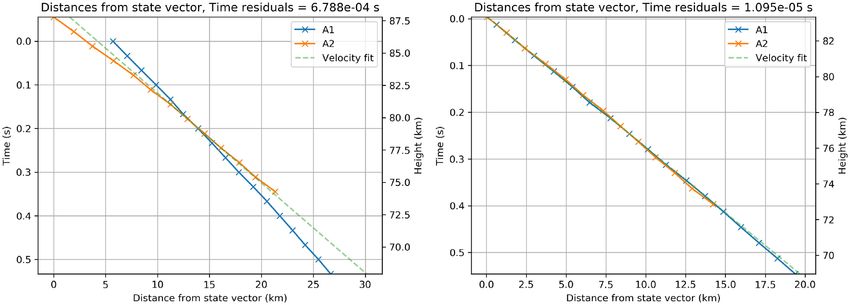
Novel meteor trajectory solver                     4005
                                                                                 due to deceleration occurring prior to detection. For this system,
                                                                                 the average underestimation is around 200 m s−1 for cometary,
                                                                                 and 300 m s−1 for asteroidal meteoroids (see Vida et al. 2018,
                                                                                 for a complete analysis). The measurement precision of the initial
                                                                                 velocity is much better, around 50 m s−1 . The accuracy of the radiant
                                                                                 estimation is approximately 0.02◦ .
                                                                                    The upper right inset of Fig. 11 shows the results obtained

                                                                                                                                                               Downloaded from https://academic.oup.com/mnras/article-abstract/491/3/3996/5645268 by University of Western Ontario user on 09 January 2020
                                                                                 using the Monte Carlo solver. Overall this solver and the LoS
                                                                                 solver provided the best precision for CAMO data. Both have
                                                                                 very low failure rates; the radiant accuracy was around 0.01◦ and
                                                                                 the geocentric velocity accuracy around 150 m s−1 . The geocentric
                                                                                 velocity was systematically underestimated due to deceleration
                                                                                 prior to detection; the accuracy could be improved by applying
                                                                                 the correction given in Vida et al. (2018).
                                                                                    The lower left inset of Fig. 11 shows simulation results using the
                                                                                 MPF method with the constant velocity model for the Draconids.
                                                                                 The geocentric velocity was underestimated more than with the
Figure 10. Comparison of geocentric radiant and velocity accuracy for the        LoS-FHAV method, as the initial velocity estimate is very heavily
simulated CAMO system for three simulated showers and various trajectory         influenced by deceleration. The average difference between the
solvers.                                                                         initial velocity and true velocity for our 100 simulated Draconids
                                                                                 was around 300 m s−1 . This difference drives the error in the radiant,
                                                                                 which had a standard deviation among our simulations of 0.04◦ .
                                                                                 For the Geminds, the velocity difference with this method was

Figure 11. Accuracy of simulated CAMO geocentric radiants for the Draconids. Upper left: Lines of sight, initial velocity estimated as the average velocity
of the first half of the trajectory. Upper right: Monte Carlo. Bottom left: Multi-parameter fit, constant velocity model. Bottom right: Multi-parameter fit,
exponential velocity model.

                                                                                                                       MNRAS 491, 3996–4011 (2020)
4006 D. Vida et al.
of convergence angles into 30 bins of equal numbers of data points;
thus 1000 simulations were needed for better statistics.
Fig. 12 shows radiant and velocity errors versus the convergence
angle, Qc , for a simulated all-sky (SOMN-like) system. Only two
stations (A1 and A2) were used for the convergence angle analysis
– when a third station is included, all maximum convergence angles
are usually >30◦ . The plotted data shows the median error value in
every bin which contains ∼33 meteors. The geometrical IP and LoS
Downloaded from https://academic.oup.com/mnras/article-abstract/491/3/3996/5645268 by University of Western Ontario user on 09 January 2020
methods produce errors on the order of degrees for Qc < 15◦ , while
the Monte Carlo and MPF methods restrict the radiant error below
1◦ even for very low values of Qc . Although the deceleration is not
directly observable for such all-sky systems, the estimated speeds
at different stations at low convergence angles do not match when
geometrical methods are used. The Monte Carlo and MPF methods,
in contrast, are designed to ‘find’ the solution which satisfies both
the spatial and dynamical constraints. As an example, Fig. 13 shows
length versus time of a low Qc synthetic Geminid estimated by the
Figure 12. Radiant and velocity error as a function of convergence angle LoS method (left inset) and the Monte Carlo method (right inset).
for 1000 Geminids simulated for an all-sky (SOMN-like) system. Note that in all the convergence angle plots, the IP and LOS-FHAV
use the same approach to compute speed and hence overlap exactly
> 1 km s−1 , which strongly indicates that using average meteor in the speed error (bottom) plots and are not separately observable
velocities is not suitable for computing orbits of asteroidal meteors. in these figures.
Finally, the lower right inset of Fig. 11 shows results obtained Next, we investigated a moderate field of view (CAMS-like) sys-
using the MPF solver with the exponential deceleration model. This tem. As with the all-sky system, only two stations were used in this
solver had a very large failure rate, above 50 per cent. The failure analysis, as three-station solutions always have large convergence
was mostly driven by the overestimation of the initial velocity; in angles. As seen in Fig. 14, all trajectory solvers have a similar radiant
contrast the estimation of the radiant position remained fairly robust. error of ∼0.1◦ for Qc > 10◦ . For smaller convergence angles, the
IP and LoS solvers produce errors on the order of 1◦ . On the other
hand, the MPF and Monte Carlo solvers produce robust radiant
3.4 Trajectory solution accuracy as a function of convergence
solutions throughout. The velocity error is less strongly correlated
angle
with the convergence angle, but is completely dominated by
The maximum convergence angle between a meteor trajectory and solver-specific biases. In particular, the MPF-exp overestimates the
stations is usually used as an indicator for the trajectory quality. initial velocity across all convergence angles, a product of the poorly
Gural (2012) has shown that the radiant error is dependent on the conditioned convergence of this kinematic model. We are roughly
convergence angle (among other factors). He found that the IP and able to reproduce the results of Jenniskens et al. (2011), where they
LoS methods produced on average a factor of 10 increase in radiant found that geometrical methods work well for Qc > 25◦ , and that
error at low (Novel meteor trajectory solver 4007
it may be a major contributor to the overall impact hazard and
supports some elements of the proposed coherent catastrophism
theory (Asher et al. 1994).
Spurnỳ et al. (2017) attribute the discovery of the Taurid branch,
linked to the swarm return in 2015, to the precision measurements
made possible by their high-resolution all-sky digital cameras and
careful manual reduction of the data. Fig. 14 in Spurnỳ et al. (2017)
Downloaded from https://academic.oup.com/mnras/article-abstract/491/3/3996/5645268 by University of Western Ontario user on 09 January 2020
shows that all meteoroids in the resonant swarm reside in a very
narrow range of semi-major axes (the extent of the 7:2 resonance
given by Asher & Clube 1993). This is arguably the strongest
evidence yet published for the real existence of the branch and
swarm as the semi-major axis is very sensitive to measurement
errors in meteor velocity. Olech et al. (2017) also noticed a possible
connection to the 7:2 resonance, but their results were not as
conclusive due to the lower measurement accuracy.
Data for the outburst have only been published for fireball-sized
meteoroids and we focus on simulating these for comparison to
Figure 14. Radiant and velocity error versus convergence angle for 1000 measurements published in Spurnỳ et al. (2017). In this section we
Geminids simulated for a moderate field of view (CAMS-like) system. investigate the precision needed to make a discovery of this nature
and discuss the limits of low-resolution all-sky systems.
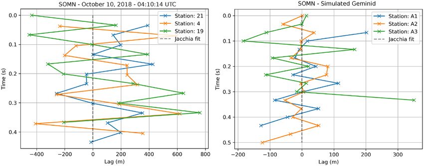
We used the parameters of the Taurid meteoroid stream resonant
branch as given in Spurnỳ et al. (2017) and simulated 100 meteors
from the branch as they would be detected by an SOMN-like all-sky
system. We only simulated meteors with the semi-major axis inside
the narrow region of the 7:2 resonance which spans 0.05 au.
Fig. 16 shows the comparison between the simulated semi-major
axes and computed values using various trajectory solvers for a three
station SOMN-like system. As can be seen, the observed scatter in
a is too large to detect the branch with any solver using such low-
quality data. This shows that existing low-resolution all-sky systems
(circa 2019) have limited utility for any orbital determination (on
a per camera basis) requiring high precision but are better suited
to shower flux estimation or meteorite recovery. Deployment of
higher resolution all-sky systems (Spurnỳ et al. 2006; Devillepoix
et al. 2018) which can achieve a radiant precision on the order
of 1 arc minute are clearly preferable for any orbit measurements
requiring high accuracy.
Figure 15. Radiant and velocity error as a function of convergence angle 3.6 Influence of gravity on trajectories of long-duration
for 1000 Geminids simulated for the CAMO system.
fireballs
The orbits of meteorite-dropping fireballs are of special interest
deceleration visible at the fine angular resolution of a CAMO- as knowing their velocities allows a statistical estimate of the
like system. Due to the limited geometry of the CAMO system, source region in the main asteroid belt and linkage to possible
the maximum expected convergence angle is less than 30◦ , but parent bodies (Granvik & Brown 2018). Because these fireballs
the solutions using the IP, LoS, and Monte Carlo solvers are very may remain luminous for long durations, often 5 or more seconds,
stable even down to Qc ∼ 1◦ . The poorer performance of the MPF- their trajectories can be precisely estimated using data even from
methods for this system, particularly in reconstructing initial speed, low-precision all-sky systems. This is due to the large number of
likely reflect the high precision of CAMO which requires a more observed points available in the data reduction. On the other hand,
physical kinematic model than the empirical models used in the these events experience the largest gravitational bending of the
MPF approach. trajectory, e.g. after 5 s the drop due to gravity is on the order of
100 m. They violate the linear trajectory assumption implicit in
many solvers. In extreme cases, Earth grazing fireballs may last for
3.5 The 2015 Taurid outburst – high-precision all-sky
tens of seconds and their path (ignoring deceleration) is a hyperbola
observations
with respect to the Earth’s surface, requiring a special approach to
In 2015, the Taurids displayed an activity outburst due to Earth solve (e.g. Ceplecha 1979; Sansom et al. 2019). Here we explore
encountering a resonant meteoroid swarm locked in a 7:2 resonance which trajectory solver is best for these long fireballs and investigate
with Jupiter (Asher & Clube 1993; Spurnỳ et al. 2017). Securing the influence of gravitational bending on the radiant precision.
accurate observations of fireballs for this resonant branch for the As the parameter space of possible radiants and lengths of
first time is significant for planetary defence as the branch was also possible meteorite-dropping fireballs is beyond the scope of this
shown to contain asteroids on the order of several 100s of meters paper, we use as a single case-study a specific fireball that was
in size. As the Earth encounters this swarm at regular intervals observed above Southwestern Ontario on September 23, 2017 by 3
MNRAS 491, 3996–4011 (2020)4008 D. Vida et al.
Downloaded from https://academic.oup.com/mnras/article-abstract/491/3/3996/5645268 by University of Western Ontario user on 09 January 2020
Figure 16. The semi-major axes of simulated 2015 Taurids from the resonant branch (blue dots bound within black dashed lines) and comparison with values
estimated using different trajectory solvers. The right plot shows a narrower range of semi-major axes.
stations of the SOMN. The fireball was first observed at 75 km and Table 8. Trajectory solver performance for a simulated
ended at 35 km, lasting 6.5 s. It entered the atmosphere at an angle long-duration fireball observed by a three station all-sky
of 30◦ from the ground and with an initial velocity of 14 km s−1 . system. The trajectory was incorporated in the simulation
Simulations were performed using the estimated radiant and the statistics if the convergence angle was larger than 5◦ – we
use a lower threshold in this case due to the larger average
velocity, but the initial positions of the fireball were randomly
duration of the event, which in turn means that there are
generated inside the fields of view of the simulated all-sky network more points for trajectory estimation. F is thepercentage
to cover a wide range of geometries. The dynamics of the fireball of failures (total of 74 meteors), i.e. thepercentage of
were simulated by using the linear deceleration meteor propagation radiants that were outside the Rmax = 0.5◦ , V max =
model. The deceleration prior to detection was not included in 0.5 km s−1 window.
the simulation because these bright fireballs do not significantly
decelerate prior to generating a visible trace in a video system Solver Fireball
(Vida et al. 2018). The duration of the fireball was set to 6.5 s, the F (%) σR σV
time of the beginning of deceleration t0 was randomly generated
IP 22% 0.18◦ 0.03 km s−1
in the range [0.3, 0.6] of the total duration of the fireball, and the LoS 8% 0.07◦ 0.02 km s−1
deceleration was randomly generated in the range [1500, 2750] LoS-FHAV 11% 0.13◦ 0.02 km s−1
m s−2 , which was comparable to the observed event, although the Monte Carlo 12% 0.09◦ 0.03 km s−1
real deceleration was of course not constant. MPF const 92% 0.32◦ 0.07 km s−1
Due to the large range of simulated starting points, not all of the MPF const-FHAV 89% 0.22◦ 0.07 km s−1
100 simulated fireballs were observed in full. Only those simulations MPF linear 50% 0.09◦ 0.02 km s−1
in which all stations observed the fireball for at least 4 s where MPF exp 88% 0.37◦ 0.24 km s−1
chosen, bringing the number down to 74 simulated meteors. Table 8
gives the comparison of the performance of various solvers applied
to this simulated data. The estimated trajectories were quite precise
because of the long duration, thus it was decided to constrain the
failure window of interest to Rmax = 0.5◦ , V max = 0.5 km s−1 . We
justify the reduction of these constraints compared to the SOMN
constraints used above by the higher number of observed points
(thus better fits), and the fact that Granvik & Brown (2018) indicate
that the precision of a fireball’s initial velocity should be estimated
to around 0.1 km s−1 for the statistical distribution of initial source
regions to be stable.
The best performing solver was the Borovička (1990) LoS
method with the initial velocity estimated using our newly proposed
sliding fit and including compensation for gravity. The expected
radiant precision is around 4 arc minutes, while the initial velocity
can be estimated to within 20 m s−1 . Fig. 17 shows the 2D histogram
of errors for all estimated trajectories. The Monte Carlo solver
performs slightly worse, but we haven’t manually chosen the
Figure 17. Accuracy of geocentric radiants for simulated fireballs. The
solution based on the existence of directionality of the ft function, solutions were done using the LoS method.
as proposed in Paper 1. On the other hand, MPF solvers have a
high failure rate, even the MPF solver with the linear deceleration
MNRAS 491, 3996–4011 (2020)Novel meteor trajectory solver 4009
Downloaded from https://academic.oup.com/mnras/article-abstract/491/3/3996/5645268 by University of Western Ontario user on 09 January 2020
Figure 19. Quality of error estimation for a CAMS-like system and 1000
Figure 18. Accuracy of geocentric radiants for a simulated long-duration Geminids.
fireball. The solutions were done using the LoS method, with the option of
compensating for the curvature due to gravity turned off.
Table 9. Parameters of fitted truncated normal and χ 2 distributions to
values of σ err for different simulated showers and systems. σ is the standard
model which should have been able to exactly estimate the trajectory
deviation of fitted truncated normal distributions (it can be considered as a
parameters.
rough proxy for the magnitude of error underestimation), and ‘k’ and ‘scale’
Next, we investigated the radiant accuracy if the compensation are parameters of the χ 2 distribution.
for the curvature due to gravity was not taken into account, i.e.
the term h(tkj ) was kept at 0 (see Paper 1 for details). Fig. 18 Shower DRA GEM PER
shows an offset of about 0.15◦ from the true radiant, caused by the σ k, scale σ k, scale σ k, scale
shift of the estimated radiant towards the local zenith. We point
out that these results were obtained on simulated data which ignore All-sky 2.37 3.23, 0.57 2.03 3.99, 0.42 2.43 4.70, 0.45
CAMS 2.02 4.61, 0.37 1.93 4.47, 0.36 2.02 6.37, 0.28
any other forces acting on the meteoroid (which are expected to be
CAMO 3.57 12.00, 0.33 3.74 4.82, 0.67 2.35 2.84, 0.61
negligible in any case), which demonstrate that the curvature of the
trajectory due to gravity should be compensated for directly during
trajectory estimation, as it otherwise produces a significant bias in
the direction of the radiant. This becomes more pronounced with the
increasing duration of the fireball. Alternatively, an analytic zenith
attraction correction could be developed (separate from the zenith
attraction correction for computing geocentric radiants) which is
dependent on the geometry and the duration of the fireball.
3.7 Estimated radiant error and true accuracy
In this final section, we investigate if the radiant error estimated
as the standard deviation from the mean accurately describes the
true magnitude of the error. We do not investigate the velocity
error estimate, because the accuracy of pre-atmosphere velocity
for smaller meteoroids is entirely driven by deceleration prior to
detection (Vida et al. 2018), causing a systematic underestimate of
top of atmosphere speeds.
Using the results of the Monte Carlo solver, we compute the Figure 20. Quality of error estimation for CAMO and 100 Draconids.
angular separation θ between the estimated and the true geocentric
radiant used as simulation input, and divide it by the hypotenuse of simulated Geminids for a CAMS-like system. We fit a truncated
standard deviations in right ascension and declination: normal distribution using the maximum-likelihood method to σ err
θ values and report standard deviations for all showers and systems
σerr = (1) in Table 9. It appears that the truncated normal distribution is not
(σα cos δ)2 + σδ2 representative of the underlying distribution of σ err values, although
The value of σ err indicates how many standard deviations from its standard deviation is a rough proxy for the scale of the error
the mean the true radiant is. In an ideal case where the errors underestimation. We also fit a χ 2 distribution which appears to be
would be correctly estimated, the distribution of σ err values for better suited (p-values are consistently high).
all trajectories would follow a truncated normal distribution with a Regarding CAMO, the real radiant errors are 2 to 4 times larger
standard deviation of one. than estimated, as seen in Fig. 20 which shows the error analysis
In practice, the errors seem to be on average underestimated by for simulated Draconids. These results indicate that for a robust
a factor two across all nine combinations of systems and showers. understanding of errors, a detailed analysis must be done for each
Fig. 19 shows the cumulative histogram of σ err values for 1000 system and shower using the shower simulator.
MNRAS 491, 3996–4011 (2020)4010 D. Vida et al.
4 CONCLUSION Simulation of the accuracy of low-precision all-sky systems with
approximately 20 arc-minute per pixel angular resolution, shows
In Paper 1 (Vida et al. 2019b), we described and implemented in
that they are not precise enough to observe structures in meteor
Python several trajectory solvers. In this paper, we have applied
showers such as the Taurid resonant branch (Spurnỳ et al. 2017). For
each solver in turn to synthetic meteors with radiants, speeds, and
accurate orbital measurements we strongly suggest installation of
physical properties appropriate to the Draconids, Geminids and the
more precise all-sky systems with angular resolutions approaching
Perseids as they would be recorded by various simulated meteor
or exceeding one arc-minute per pixel so that the velocity accuracy
observation systems. While we have generically investigated solver
of less than 0.1 km s−1 can be achieved, as recommended by
Downloaded from https://academic.oup.com/mnras/article-abstract/491/3/3996/5645268 by University of Western Ontario user on 09 January 2020
performance for common optical systems, the simulator allows
Granvik & Brown (2018). We show that compensation for trajectory
for detailed simulation of individual real-world meteor observing
bending due to gravity should be taken into account for longer
systems and estimation of the measurement accuracy of meteor
fireballs (>4 seconds) due to its significant influence on the radiant
showers or individual events of interest. While we summarize
accuracy, as noted earlier by Ceplecha (1979) and Sansom et al.
some major trends of our simulation comparisons, it is important
(2019).
to emphasize that these results pertain only to the geometry and
Finally, we investigated the quality of our radiant error estima-
number of cameras assumed for each simulated system and shower.
tion approach by comparing estimated errors to known absolute
Ideally, for real observations, simulations would be repeated for
error from the simulation input. We find that radiant errors are
specific geometries and camera systems on a per event basis.
underestimated by a factor of 2 for all-sky and CAMS-like systems,
With this caveat in mind, based on our simulations, the following
and by a factor of 3 to 4 for CAMO.
is a summary of which trajectory solver performed best for our
chosen showers for each meteor observation system:
4.1 Note on code availability
(i) All-sky systems (SOMN-like) – As meteor deceleration is not
usually seen by these systems, the MPF method with the constant Implementation of the meteor simulator as well as implementation
velocity model produces the most robust fits and estimates radiants of all meteor solvers used in this work are published as open source
the most precisely, to within 0.25◦ . The method significantly on the following GitHub web page: https://github.com/wmpg/West
underestimates the initial velocity, but if a correct deceleration ernMeteorPyLib. Readers are encouraged to contact the authors in
correction is applied an accuracy of ∼250 m s−1 could be achieved. the event they are not able to obtain the code on-line.
(ii) Moderate field of view systems (CAMS-like) – The in-
tersecting planes and the lines of sight methods produce good
results overall when employed in conjunction with more advanced 5 S I M U L AT I O N O R B I T R E P O RT S
methods of initial velocity estimation, because meteor deceleration
In supplementary files, we provide all trajectory and orbit report
becomes visible at the resolutions of such systems. The Monte Carlo
files of simulated trajectories used in this paper. The report files
solver results are comparable to these solvers and does not provide
include all inputs to the solver, as well as all trajectory and orbit
further improvement of the solution except for meteors with low
parameters. We encourage readers to use these values to verify their
convergence angles. We recommend using this solver operationally
implementations of the method.
for these systems. The MPF methods improve the radiant precision,
but their estimates of the initial velocity are a factor or 2 worse
than with other methods. The expected average radiant and velocity AC K N OW L E D G E M E N T S
accuracy is around 0.1◦ and 100 m s−1 , provided the pre-detection
deceleration correction from Vida et al. (2018) is used. We thank Dr. Eleanor Sansom for a helpful and detailed review of an
(iii) The CAMO, high-precision system which observes meteor earlier version of this manuscript. Also, we thank Dr. Auriane Egal
dynamics (deceleration) well – The Monte Carlo and LoS solvers for suggestions about the modelling of the Draconids. Funding for
perform the best. The expected average radiant accuracy is around this work was provided by the NASA Meteoroid Environment Office
0.01◦ and 50 m s−1 , provided the pre-detection deceleration correc- under cooperative agreement 80NSSC18M0046. PGB acknowl-
tion from Vida et al. (2018) is used. The MPF approach enforces edges funding support from the Canada Research Chair program
meteor propagation models which are mismatched to the actual and the Natural Sciences and Engineering Research Council of
deceleration behaviour, resulting in fits with larger errors for these Canada.
high angular and temporal resolution measurements.
(iv) Meteoroid physical properties strongly influence the velocity
REFERENCES
accuracy. Meteoroids of asteroidal origin have a factor of 2 higher
velocity uncertainties due to larger deceleration, a conclusion Asher D., Clube S., 1993, Q. J. R. Astron. Soc., 34, 481
previously reported in Vida et al. (2018). Asher D., Clube S., Napier W., Steel D., 1994, Vistas Astron., 38, 1
Beech M., 2002, MNRAS, 336, 559
We show that a minimum radiant accuracy of order 3 to 6 Beech M., Nikolova S., 1999, Meteorit. Planet. Sci., 34, 849
arc minutes (0.05◦ – 0.1◦ ) is needed to measure the true radiant Blaauw R., Campbell-Brown M., Weryk R., 2011, MNRAS, 414, 3322
dispersion of younger meteor showers. This value was derived by Borovička J., 1990, Bull. Astron. Inst. Czech., 41, 391
Borovička J., Koten P., Shrbenỳ L., Štork R., Hornoch K., 2014, Earth,
simulating the 2011 Draconids outburst, a year where the encounter
Moon, and Planets, 113, 15
with recently ejected meteoroids having a very low dispersion. With
Borovička J., Koten P., Spurnỳ P., Čapek D., Shrbenỳ L., Štork R., 2009,
the use of an appropriate trajectory solver, this accuracy can be Proc. Int. Astron. Union, 5, 218
achieved using moderate FOV and CAMO resolution systems, i.e. Borovička J., Spurnỳ P., Koten P., 2007, A&A, 473, 661
systems with the angular resolution better than 3 arc-minutes per Brown P., Jones J., 1998, Icarus, 133, 36
pixel (assuming a real precision of around 1 arc-minute is achievable Brown P., Marchenko V., Moser D. E., Weryk R., Cooke W., 2013, Meteorit.
through centroiding). Planet. Sci., 48, 270
MNRAS 491, 3996–4011 (2020)You can also read