Deep Manifold Learning for Dynamic MR Imaging
←
→
Page content transcription
If your browser does not render page correctly, please read the page content below
Deep Manifold Learning for Dynamic MR Imaging
                                          Ziwen Ke 1, 2, † , Zhuo-Xu Cui 3, † , Wenqi Huang 1, 2 , Jing Cheng 3 , Sen Jia 3 , Haifeng
                                          Wang 3 , Xin Liu 3 , Hairong Zheng 3 , Leslie Ying 4 , Yanjie Zhu 3 , Dong Liang 1, *

                                          1 Research Center for Medical AI, Shenzhen Institutes of Advanced
                                          Technology, Chinese Academy of Sciences, Shenzhen, China
                                          2 Shenzhen College of Advanced Technology, University of Chinese
arXiv:2104.01102v1 [eess.IV] 9 Mar 2021

                                          Academy of Sciences, Shenzhen, China
                                          3 Paul C. Lauterbur Research Center for Biomedical Imaging, Shenzhen
                                          Institutes of Advanced Technology, Chinese Academy of Sciences,
                                          Shenzhen, China
                                          4 Department of Biomedical Engineering and the Department of Electrical
                                          Engineering, The State University of New York, Buffalo, NY, USA

                                          †: These authors contributed equally to this work.
                                          * Corresponding author:
                                                  Name Dong Liang
                                            Department Research Center for Medical AI
                                               Institute Shenzhen Institutes of Advanced Technology, Chinese Academy of
                                                Address 1068 Xueyuan Avenue, Shenzhen University Town
                                                         Shenzhen
                                                         China
                                                 E-mail dong.liang@siat.ac.cn

                                          Abstract
                                          Purpose: To develop a deep learning method on a nonlinear manifold to explore the
                                          temporal redundancy of dynamic signals to reconstruct cardiac MRI data from highly
                                          undersampled measurements.
                                              Methods: Cardiac MR image reconstruction is modeled as general compressed
                                          sensing (CS) based optimization on a low-rank tensor manifold. The nonlinear manifold
                                          is designed to characterize the temporal correlation of dynamic signals. Iterative
                                          procedures can be obtained by solving the optimization model on the manifold,
                                          including gradient calculation, projection of the gradient to tangent space, and
                                          retraction of the tangent space to the manifold. The iterative procedures on the
                                          manifold are unrolled to a neural network, dubbed as Manifold-Net. The Manifold-Net
                                          is trained using in vivo data with a retrospective electrocardiogram (ECG)-gated
                                          segmented bSSFP sequence.
                                              Results: Experimental results at high accelerations demonstrate that the proposed
                                          method can obtain improved reconstruction compared with a compressed sensing (CS)
                                          method k-t SLR and two state-of-the-art deep learning-based methods, DC-CNN and
                                          CRNN.
                                              Conclusion: This work represents the first study unrolling the optimization on
                                          manifolds into neural networks. Specifically, the designed low-rank manifold provides a
                                          new technical route for applying low-rank priors in dynamic MR imaging.

                                                                                                                                1/17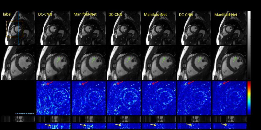
1    Introduction
In 2019, ischaemic heart disease was the 1st leading cause of death worldwide,
responsible for 16% of the world’s total deaths [1]. Many imaging modalities, namely,
magnetic resonance imaging (MRI), computed tomography (CT), and ultrasonic, are
employed for heart diagnosis. The key to the diagnosis is whether the imaging methods
can capture the cardiac structure and dynamic motion. Of these modalities, not only is
MRI free from ionizing radiation and the use of radioactive tracers, but also with
unparalleled soft-tissue contrast and high spatial resolution. However, MRI has yet to
become a routine part of clinical workup in cardiac patients [2], primarily due to the
limitation: speed. The acquisition time would increase significantly if the more excellent
spatial resolution, volume coverage, and motion-corrupted acquisitions are needed. To
overcome this limitation, acceleration methods from highly under-sampled k-space
measurements have been intensely studied for nearly three decades.
    Accelerated dynamic MRI is unique because of an extra time dimension. Exploration
of the Spatio-temporal correlation of dynamic signals plays an essential role in
maximizing acceleration. k-t accelerated imaging [3–6] is one of the earliest acceleration
methods that reduce the reconstruction problem to a mathematical estimation via a
linear combination of acquired points in k-t space. To capture and utilize global
similarities for ensuring more accurate reconstruction, compressed sensing (CS) [7–9]
has been utilized. According to CS, incoherent artifacts from random undersampling
can be removed in some transform (sparse basis) domains by nonlinear reconstruction.
From the initial fixed basis [10–12], to the sparse adaptive basis [13–15], and then to the
recent use of a neural network to learn the sparse basis [16–19], the sparse prior in CS is
more and more intelligent with continuously improved reconstruction performance.
    Recently, manifold learning [20–23] has achieved some success in accelerated cardiac
MRI. The core of manifold learning is an assumption that the dynamic signals in high
dimensional space are adjacent points on smooth and low dimensional manifolds. The
construction of low-dimensional manifolds is a topic of ongoing research. For example,
in SToRM [20], a graph Laplacian matrix is established from a navigator acquisition
scheme to determine the structure of the manifold. KLR [21] used kernel principal
component analysis (KPCA) [24] to learn the manifold described by the principal
components of the feature space. BiLMDM [22] extracted a set of landmark points from
data by a bi-linear model to learn a latent manifold geometry. These methods posed the
manifold smoothness prior as a regularization in a CS optimization problem and
performed iterative optimization in the linear European space to obtain reconstructed
results. Although these works make generous contributions to dynamic MRI, the
following issues still need to be addressed: 1) the manifold smoothness prior is located
in nonlinear manifolds, while corresponding iterative optimization is not performed
along with the nonlinear structure of the manifold; 2) Manifold regularization, as an
extension of CS, cannot escape the essential iterative reconstruction process, and cannot
avoid tedious reconstruction time and parameter selection.
    Inspired by Riemannian optimization [25, 26], we propose a deep manifold learning
for dynamic MRI in this paper. In particular, a low-rank tensor manifold is designed to
characterize the strong temporal correlation of dynamic signals. Dynamic MR
reconstruction is modeled as a general CS-based optimization on the manifold.
Riemannian optimization on the manifold is used to solve this problem, and iterative
procedures can be obtained. To avoid the disadvantages of long iterative solution time
and difficult parameter selection, these iterative procedures are unrolled into a neural
network, dubbed as Manifold-Net. Extensive experiments on in vivo MRI data illustrate
noteworthy improvements of the proposed Manifold-Net over state-of-the-art
reconstruction techniques. This work represents the first study unrolling the
optimization on manifolds into neural networks. Besides, the designed low-rank manifold

                                                                                      2/17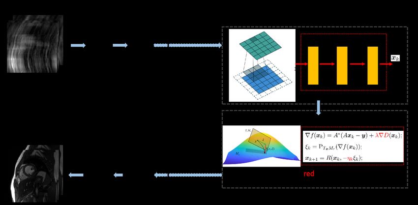
provides a new technical route for applying low-rank priors in dynamic MR imaging.
   The rest of this paper is organized as follows. Section II and III provide the recall of
Riemannian optimization theory and introduces the proposed methods. Section IV
summarizes the experimental details and the results to demonstrate the effectiveness of
the proposed method, while the discussion and conclusions are presented in Section IV
and V, respectively.

2     Theory
Tensor completion [27] fills in missing entries of a partially known tensor with a
low-rank constraint. Riemannian optimization techniques on a manifold of tensors of
fixed rank have been mathematically and experimentally proved feasible to solve the
tensor completion problem [26]—this section recall Riemann optimization theory.
Detailed introduction of theoretical derivation is beyond the scope of this paper, so we
focus on its three important iterative steps: gradient calculation, projection of the
gradient to tangent space, and retraction of the tangent space to the manifold.
Throughout this section, we follow the notation in [26].

2.1    Preliminaries on Tensors
    • T he ith mode matricization:
      The ith mode matricization of a tensor x ∈ Cn1 ×···×nd is a rearrangement of the
      entries of x into the matrix x(i) , such that the ith mode becomes the row index
      and all other (d − 1) modes become column indices, in lexicographical order.

                                         x(i) ∈ Cni ×Πj6=i nj                                   (1)

    • T he multilinear rank:
      The ranks of all the mode matricizations yield the multilinear rank tuple r of x:

                       rank(x) = (rank(x(1) ), rank(x(2) ), . . . , rank(x(d) ))                (2)

    • T he ith mode product:
      The ith mode product of x multiplied with a matrix M ∈ Cm×ni is defined as

                                 y = x ×i M ⇔ y(i) = M x(i) ,
                                                                                                (3)
                                 y ∈ Cn1 ×···×nn−1 ×m×ni+1 ×···×nd

    • T ucker decomposition:
      Any tensor of multilinear rank of r = (r1 , r2 , . . . , rd ) can be represented in the
      so-called T ucker decomposition
                                                                    d
                             x = C ×1 U1 ×2 U2 · · · ×d Ud = C × Ui                             (4)
                                                                   i=1

      with the core tensor C ∈ Cr1 ×···×rd , and the basis matrices Ui ∈ Cni ×ri .
      Without loss of generality, all Ui are orthonormal: UiT Ui = Iri .
    • Higher order singular value decomposition:
      The truncation of a tensor x to a fixed rank r can be obtained by the higher order
      singular value decomposition (HOSVD) [28], denoted as PHO  r . The HOSVD

                                                                                           3/17
procedure can be described by the successive application of best rank-ri
approximations Piri in each mode i = 1, . . . , d:
PHO
r : Cn1 ×···×nd → Mr , x 7→ Pdrd ◦ · · · ◦ P1r1 x. (5)
Each individual projection can be computed by a truncated SVD as follows. Let
UY contain the ri dominant left singular vectors of the ith matricization Y(i) of a
given tensor y. Then the tensor resulting from the projection ỹ = Piri y is given in
terms of its matricization as Ỹ(i) = UY UYT Y(i) . The HOSVD does inherit the
smoothness of low-rank matrix approximations [29].
2.2 Manifold setting
The set Mr of tensors of fixed rank r = (r1 , r2 , . . . , rd ) forms a smooth embedded
submanifold of Cn1 ×···×nd [30]. By counting the degrees of freedom in (4), it follows
that the dimension of Mr is given by
d
Y d
X
dim(Mr ) = rj + ri ni − ri2 (6)
j=1 i=1
According to [31], the tangent space of Mr at x = C ×1 U1 ×2 U2 · · · ×d Ud can be
parametrized as
( d
)
d X
Tx Mr = G × Ui + C ×i Vi × Uj |ViT Ui = 0 (7)
i=1 j6=i
i=1
where G ∈ Cr1 ×···×rd and Vi ∈ Cni ×ri are the free parameters. Furthermore, the
orthogonal projection of a tensor A ∈ Cn1 ×···×nd onto Tx Mr is given by
PTx Mr : Cn1 ×···×nd → Tx Mr
d d
A 7→ A × UjT × Ui
j=1 i=1 (8)
d !
X 1 T †
+ C ×i P A × Uj C(i) × Uk
i=1
Ui j6=i (i) k6=i
†
Here C(i) denotes the pseudo-inverse of C(i) . Note that C(i) has been full row rank and
† T −1
hence C(i) T
= C(i) (C(i) C(i) ) . We use P U1i := Iri − Ui UiT to denote the orthogonal
projection onto the orthogonal complement of span(Ui ).
2.3 Riemanian Gradient and Retraction
As a metric on Mr , the Euclidean metric from the embedded space induced by the inner
product (3). Together with this metric, Mr becomes a Riemannian manifold. This, in
turn, allows us to define the Riemannian gradient of an objective function, which can be
obtained from the projection of the Euclidean gradient into the tangent space.
Let f : Cn1 ×···×nd be a cost function with Euclidean gradient ∇fx at point x ∈ Mr .
The Riemannian gradient [25] of f : Mr → C is given by
grad f (x) = PTx Mr (∇fx ) (9)
Let ξ := −grad f (x) be Riemannian gradient update.
4/17Retraction R : Tx Mr → Mr maps an element from the tangent space at x ∈ Mr to
the manifold Mr . HOSVD is chosen to implement the retraction:
R : Tx Mr , (x, ξ) 7→ PHO
r (x + ξ) (10)
A graphical depiction of these concepts is shown in Fig. 1.
Figure 1. Graphical representation of the concept of Riemannian gradient, retraction
and update on the manifold within the framework of Riemannian optimization techniques.
3 Methods
3.1 Problem Formulation
The reconstruction of dynamic MR images from under-sampled k-space data can be
described as a tensor completion problem. Namely, given only under-sampled k-space
data, it is required to reconstruct the full-sampled MR image. However, the completion
process is ill-conditioned; that is, there are multiple solutions that are consistent with
under-sampled data. To reduce the range of solutions and stabilize the solution
procedure, regularization is a common strategy. In consideration of the strong
correlation between adjacent frames, the low-rank constraint is introduced to achieve
regularization for dynamic MR imaging [32–36]. This yields a nonlinear optimization
problem as follows:
1
min kAx − yk2 + λD(x), s.t. rank(x) = r (11)
x∈CNx Ny Nt 2
Where A = P F is the encoding operator, F denotes the Fourier transform, and P
denotes an under-sampling operator, DP is used to regularize each slice of x. In
T
particular, D can be usually chosen as t=1 kW xt k1 , where W denotes a certain
sparsifying transform, such as wavelet, gradient mapping, etc.
For r-rank constrained optimization problem, iterative hard thresholding
method [37] is the most common method:
rk+1 =xk − ηk (A∗ (Axk − y) + λ∇D(xk ))
(12)
xk+1 =PHO
r (rk+1 )
where PHO
r denotes the higher-order singular value decomposition (HOSVD) operator
(5). The above hard algorithm can be regarded as gradient descent (GD) step
compound with a hard thresholding mapping. GD is performed on Euclidean space , so
5/17rk+1 does not have rank r. An additional hard thresholding mapping is added to ensure
that the iterate satisfies the r-rank constraint.
Since the GD step is only focused on seeking the direction towards an optimal
solution on Euclidean space rather than low-rank constraint set and neglects the
low-rank structure of seeking solutions, which usually leads to slow convergence of hard
algorithms [26]. Furthermore, in this paper, we propose to design an effective
optimization unrolled method for the problem (11). Due to the limitation of computing
capacity, the number of network layers of optimization unrolled method is usually
chosen far less than the number of iterations of the traditional iterative algorithm.
Therefore, the algorithms with slow convergence are not suitable for unrolling.
On the other hand, recent researches show that the set of tensors of fixed multilinear
rank r forms a smooth manifold [26]. From this point of view, the low-rank constrained
optimization problem (11) reduces to an unconstrained optimization problem on a rank
r tensor formed manifold Mr :
1
min f (x) := kAx − yk2 + λD(x) (13)
x∈Mr 2
By exploiting the manifold structure of Mr , it allows for the use of Riemannian
optimization techniques.
3.2 Riemannian Optimization
To solve the Riemannian optimization problem (13), Riemannian GD (GD restricted to
Mr ) is one of the simplest and most effective schemes. The main difference from a hard
algorithm is that every iterate of Riemannian GD always stays on the manifold Mr and
the calculations of gradient and iterative trajectory always follows the manifold
structure itself.
Starting with the initial point x0 ∈ Mr , there are following two main steps to
executing the Riemannian GD: 1) calculate Riemannian gradient and 2) iterate on
manifold along the direction of negative gradient. Because of the nonlinearity of
manifolds, the gradient of f is generalized as a point to the direction for greatest
increase within the tangent space Tx Mr , which in detail reads:
gradf (x) := PTx Mr (A∗ (Ax − y) + λ∇D(x)) where PTx Mr denotes a projection onto the
tangent space Tx Mr . The detailed calculation of Riemann gradient on manifold Mr is
shown in (8).
Unlike Euclidean space, one point moving in the direction of the negative
Riemannian gradient is not guaranteed to always fall into manifold Mr . Hence, we will
need the concept of a retraction R which maps the new iterate x + ηξ back to a point
R(x, ηξ) in manifold Mr . The detailed calculation of retraction mapping on manifold
Mr is shown in (10). The main iterative process of Riemannian GD is shown in the
Algorithm 1.
Algorithm 1 Riemannian GD for problem (13).
1: Input: K ≥ 1 and sequences {ηk }Tk=1 ;
2: Initialize: x0 ∈ Mr ;
3: for k = 1, . . . , T do
4: ∇f (xk ) = A∗ (Axk − y) + λ∇D(xk );
5: ξk = PTx Mr (∇f (xk ));
6: xk+1 = R(xk , −ηk ξk );
7: end for
8: Output: xK .
6/173.3 The Proposed Network
Although the iterative scheme of Riemannian GD for the problem (13) was given, there
are two intractable problems: both the hyper-parameters {λ, ηk } and regularizer D(·)
need to be selected empirically, which is tedious and uncertain. What’s worse, the
iterative solution often takes a long time, which limits its clinical application.
To address the above two issues, we propose a deep Riemannian network, dubbed as
Manifold-Net. Manifold-Net is composed of multiple cascaded neural network blocks
depicted in Fig. 2. Each block contains a convolution module and a Riemannian
optimization module. The convolution module is made up of three convolution layers
for feature extraction. The Riemannian optimization module unrolls Algorithm 1 into a
deep neural network. Specifically, the three procedures participate in the forward
process of the network, the hyperparameters {λ, ηk } and regularizer D(·) are set to be
learnable by the network. Among them, the hyperparameters are defined as the
learnable variables of the network, and the regularizer is learned by the convolutional
neural networks.
Our proposed deep Manifold-Net has the following advantages: 1) Every iteration of
the Riemannian network always stays on the manifold Mr , and the calculations of
gradient and iterative trajectory always follows the manifold structure itself. 2). The
proposed network can learn all of the hyperparameters and transforms, which eliminates
the complex and lengthy selection of parameters and transforms. 3). Once the optimal
network parameters are learned, we can reconstruct images with good quality in
seconds, as the network avoids the tedious iteration associated with traditional low-rank
dynamic MRI. This work represents the first study unrolling the optimization on
manifolds into neural networks.
Figure 2. The proposed Manifold-Net based on Riemannian optimization. Manifold-Net
is composed of multiple cascaded neural network blocks. Each block contains convolution
and Riemannian optimization.
7/174 Results
4.1 Setup
4.1.1 Data acquisition
The fully sampled cardiac cine data were collected from 30 healthy volunteers on a 3T
scanner (MAGNETOM Trio, Siemens Healthcare, Erlangen, Germany) with a
20-channel receiver coil array. All in vivo experiments were approved by the
Institutional Review Board (IRB) of Shenzhen Institutes of Advanced Technology, and
informed consent was obtained from each volunteer. Relevant image parameters of our
cine sequence included the following. For each subject, 10 to 13 short-axis slices were
imaged with the retrospective electrocardiogram (ECG)-gated segmented bSSFP
sequence during breath-hold. A total of 386 slices were collected. The following
sequence parameters were used: FOV = 330 × 330 mm, acquisition matrix = 256 × 256,
slice thickness = 6 mm, and TR/TE = 3.0 ms/1.5 ms. The acquired temporal
resolution was 40.0 ms and reconstructed to produce 25 phases to cover the entire
cardiac cycle. The raw multi-coil data of each frame were combined by an adaptive coil
combine method [38] to produce a single-coil complex-valued image. We randomly
selected images from 25 volunteers for training and the rest for testing. Deep learning
typically requires a large amount of data for training [39]. Therefore, we applied data
augmentation using rigid transformation-shearing to enlarge the training pool. We
sheared the dynamic images along the x, y, and t directions. The sheared size was
192 × 192 × 18 (x × y × t), and the stride along the three directions was 25, 25, and 7.
Finally, we obtained 800 2D-t cardiac MR data of size 192 × 192 × 18 (x × y × t) for
training and 118 data for testing.
Retrospective undersampling was performed to generate input/output pairs for
network training. We fully sampled frequency encodes (along with kx ) and randomly
undersampled phase encodes (along ky ) according to a zero-mean Gaussian variable
density function [11] as shown in Fig 3. Wherein four central phase encodes were
ensured to be sampled.
Figure 3. The undersampling masks used in this work. (a) Label. (b) Gaussian
random mask (8-fold). (c) Zero-filling image (Gaussian, 8-fold). (d) Gaussian random
mask (12-fold). (e) Zero-filling image (Gaussian, 12-fold). (f) Vista mask (8-fold). (g)
Zero-filling image (Vista, 8-fold). (h) Radial mask (8-fold). (i) Zero-filling image (Radial,
8-fold). (j) Spiral mask (8-fold). (k) Zero-filling image (Spiral, 8-fold).
8/174.1.2 Model configuration
To demonstrate the effectiveness and flexibility of the Manifold-Net in dynamic MR cine
imaging, we compared the results of Manifold-Net with the single-coil version of a
CS-based method (k-t SLR [34]) and two state-of-the-art CNN-based methods
(DC-CNN [16], and CRNN [17]). We did not compare with MoDL-SToRM [19] since the
SToRM acquisition relied on navigator signals that were used to compute the manifold
Laplacian matrix, while we acquired the data without a navigator and its source code is
not publicly available. All comparison methods were executed according to the source
code provided by the authors. For a fair comparison, all the methods mentioned in this
paper were adjusted to their best performance.
We divided each data into two channels for network training, where the channels
stored real and imaginary parts of the data. Therefore, the inputs of the network were
undersampled k-space C2Nx Ny Nt , and the outputs were reconstruction images
C2Nx Ny Nt . Manifold-Net has ten iterative steps; that is, K = 10. The rank selection of
a fixed-rank manifold is 13; that is r = 13. The learned transforms, {D}, are different
for each layer. Each convolutional layer had 32 convolution kernels, and the size of each
convolution kernel was 3 × 3 × 3. He initialization [40] was used to initialize the network
weights. Rectifier linear units (ReLU) [41] were selected as the nonlinear activation
functions. The mini-batch size was 1. The exponential decay learning rate [42] was used
in all CNN-based experiments with an initial learning rate of 0.001 and a decay of 0.95.
All the models were trained by the Adam optimizer [43] with parameters β1 = 0.9,
β2 = 0.999, and = 10−8 to minimize a mean square error (MSE) loss function. Code is
available at https://github.com/Keziwen/Manifold_Net.
The models were implemented on an Ubuntu 16.04 LTS (64-bit) operating system
equipped with an Intel Xeon Gold 5120 central processing unit (CPU) and an Nvidia
RTX 8000 graphics processing unit (GPU, 48 GB memory) in the open framework
TensorFlow [44] with CUDA and CUDNN support. The network training took
approximately 36 hours within 50 epochs.
4.1.3 Performance evaluation
For a quantitative evaluation, the MSE, peak-signal-to-noise ratio (PSNR), and
structural similarity index (SSIM) [45] were measured as follows:
MSE = ||Ref − Rec||22 (14)
√
max(Ref ) N
PSNR = 20 log10 (15)
||Ref − Rec||2
SSIM = l(Ref, Rec) · c(Ref, Rec) · s(Ref, Rec) (16)
where Rec is the reconstructed image, Ref denotes the reference image, and N is the
total number of image pixels. The SSIM index is a multiplicative combination of the
luminance term, the contrast term, and the structural term (details are shown in [45]).
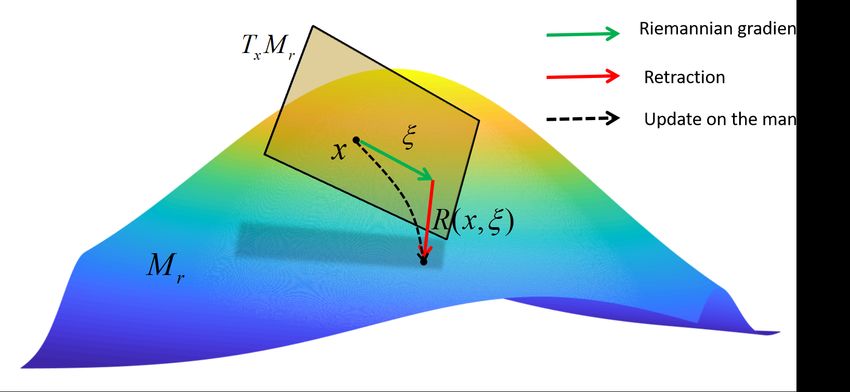
4.2 The Reconstruction Performance of the Proposed
Manifold-Net
To demonstrate the efficacy of the proposed Manifold-Net in the single-coil scenario, we
compared it with a CS-LR method; namely, k-t SLR [34], and two sparse-based CNN
methods, namely, DC-CNN [16], and CRNN [17]. The reconstruction results of these
methods at 8-fold acceleration are shown in Fig.4. The first row shows, from left to
9/17right, the ground truth and the reconstruction results of the methods as marked in the
figure. The second row shows the enlarged view of the corresponding heart regions
framed by a yellow box. The third row shows the error map (display ranges [0, 0.07]).
The y-t image (extraction of the 124th slice along the y and temporal dimensions, as
marked by the blue dotted line), and the error of the y-t image are also given for each
signal to show the reconstruction performance in the temporal dimension. The
reconstruction performance of the three deep learning-based methods (DC-CNN,
CRNN, and Manifold-Net) is better than that of the traditional iterative method (k-t
SLR), which can be clearly seen from the error maps. The comparison between the
three deep learning methods shows that Manifold-Net is better than the other three
methods in both detail retention and artifact removal (as shown by the green and red
arrows). The y-t results also have consistent conclusions, as shown by the yellow arrows.
The numbers of parameters for these network models are provided in Table 1.
Manifold-Net has the minimum number of parameters, so it can be concluded that
Manifold-Net gets the optimal reconstruction results due to the deep learning-based
Riemannian optimization rather than a larger network capacity.
Figure 4. The reconstruction results of the different methods (k-t SLR, DC-CNN,
CRNN, and the proposed Manifold-Net) at 8-fold acceleration. The first row shows,
from left to right, the ground truth and the reconstruction results of these methods.
The second row shows the enlarged view of their respective heart regions framed by a
yellow box. The third row shows the error map (display ranges [0, 0.07]). The y-t image
(extraction of the 124th slice along the y and temporal dimensions, as marked by the
blue dotted line) and the error of y-t image are also given for each signal to show the
reconstruction performance in the temporal dimension.
We also provide quantitative evaluations (MSE, PSNR, SSIM) in Table 1.
Manifold-Net achieves optimal quantitative evaluations (MSE, PSNR, and SSIM). Both
qualitative and quantitative results demonstrate that the proposed Manifold-Net can
effectively explore the low-rank prior of dynamic data, thus improving the
reconstruction performance. It is also proved that the deep learning-based optimization
on manifolds is feasible.
10/17Table 1. The average MSE, PSNR, SSIM of k-t SLR, DC-CNN, CRNN and Manifold-
Net on the test dataset at 8-fold acceleration (mean±std).
Methods MSE(*e-5) PSNR SSIM(*e-2) Parameters(*e+4)
k-t SLR 8.22 ± 3.04 41.14 ± 1.57 95.11 ± 0.88 /
DC-CNN 7.43 ± 2.33 41.48 ± 1.30 96.22 ± 0.76 43.2650
CRNN 5.60 ± 1.67 42.70 ± 1.24 97.07 ± 0.61 29.7794
Manifold-Net 3.50 ± 0.58 44.62 ± 0.77 97.95 ± 0.31 11.2325
5 Discussion
5.1 Higher Acceleration: 12-fold
The proposed method can explore the low-rank priors of dynamic signals on the
manifold, which not only improves the reconstruction performance but also increases
the acceleration rate because more expert knowledge is introduced into the optimization
problem. We explore the reconstruction performance at higher accelerations in a
single-coil scenario. The 12-fold accelerated reconstruction results can be found in Fig.
5. Our proposed Manifold-Net still achieves superior reconstruction performance at
12-fold acceleration. Although the results are slightly vague, most of the details are well
preserved. The quantitative indicators are provided in Table 2, which confirms that our
proposed Manifold-Net still achieves excellent quantitative performance at higher
accelerations.
Figure 5. The reconstruction results of the proposed Manifold-Net at 12-fold accelera-
tions in the single-coil scenario. The first row shows, from left to right, the ground truth
and the reconstruction results of these methods. The second row shows the enlarged
views of their respective heart regions framed by a yellow box. The third row shows the
error maps (display ranges [0, 0.07]). The y-t image (extraction of the 124th slice along
the y and temporal dimensions, as marked by the blue dotted line) and the error of the
y-t image are also given for each signal to show the reconstruction performance in the
temporal dimension.
11/17Table 2. The average MSE, PSNR, SSIM of k-t SLR, DC-CNN, CRNN and Manifold-
Net on the test dataset at 12-fold acceleration (mean±std).
Methods MSE(*e-5) PSNR SSIM(*e-2)
k-t SLR 14.66 ± 6.62 38.76 ± 1.91 91.71 ± 2.52
DC-CNN 12.98 ± 3.62 39.03 ± 1.19 93.78 ± 0.87
CRNN 11.87 ± 3.35 39.43 ± 1.21 94.57 ± 0.89
Manifold-Net 6.46 ± 0.97 41.95 ± 0.67 96.37 ± 0.40
5.2 The Sensitivity to Different Undersampling Masks
The proposed Manifold-Net has good reconstruction performance for different
undersampling masks. In this section, as a proof-of-concept, we explored the results of
Manifold-Net trained under different masks (radial [46], spiral [47], and VISTA [48]) at
8-fold acceleration. The reconstruction results under different undersampling masks can
be found in Fig. 6. Compared with DC-CNN [16], the proposed Manifold-Net achieves
better reconstruction results regardless of the mask, as shown by the red arrow.
Especially under the VISTA undersampling mask, the reconstruction results of
DC-CNN-Net are significantly poorer than those of radial and spiral methods. However,
Manifold-Net still maintains good reconstruction results. The quantitative indicators,
shown in Table 3, confirm that our proposed Manifold-Net achieves better quantitative
performance under each undersampling mask.
Figure 6. The reconstruction results of the proposed Manifold-Net under different
undersampling masks (radial, spiral, and VISTA) at 8-fold acceleration.
5.3 The Rank Selection: r
We designed a fixed rank manifold, Mr , to describe the temporal redundancy of
dynamic signals. The selection of rank greatly influences the reconstruction
performance, which is discussed in this section. The quantitative indicators under
different ranks are given in Fig. 7. The best reconstruction performance is achieved
when the rank r is equal to 13. As the rank gets smaller, the reconstruction gets worse.
This indicates that when the rank is 13, the designed manifold can well describe the
temporal redundancy of the dynamic signals.
12/17Table 3. The average MSE, PSNR and SSIM of DC-CNN and Manifold-Net under
different undersampling masks at 8-fold acceleration on the test dataset (mean±std).
Methods MSE(*e-5) PSNR SSIM(*e-2)
DC-CNN 12.02 ± 3.83 39.43 ± 1.43 92.71 ± 1.32
Vista Manifold-Net 5.64 ± 0.84 42.53 ± 0.63 96.34 ± 0.45
DC-CNN 5.46 ± 1.91 42.88 ± 1.49 96.84 ± 0.83
Radial Manifold-Net 2.58 ± 0.42 45.94 ± 0.73 98.38 ± 0.24
DC-CNN 4.05 ± 1.41 44.17 ± 1.46 97.50 ± 0.68
Spiral Manifold-Net 2.15 ± 0.32 46.73 ± 0.67 98.60 ± 0.21
Figure 7. The average MSE, PSNR, SSIM of Manifold-Net under different ranks on
the test dataset at 8-fold acceleration. (a) MSE. (b) PSNR. (c) SSIM.
5.4 The Limitations of the Proposed Manifold-Net
Although the Manifold-Net achieves improved reconstruction results, it still has the
following limitations: 1) Fixed-rank manifolds need to be characterized in advance,
especially the selection of rank r. If the rank selection is not good, the reconstruction
performance may be poor. 2) MRI is collected in multiple coils. Still, this paper only
discusses the results in the single-coil scenario, and the effectiveness of the multi-coil
version of Manifold-Net remains to be verified. 3) Due to the application of HOSVD in
the Riemannian optimization, the reconstruction time reached 5-6s for the entire 18
frames of dynamic signals. An SVD-free strategy [49] will be explored in future work.
6 Conclusions
This paper develops a deep learning method on a nonlinear manifold to explore the
temporal redundancy of dynamic signals to reconstruct cardiac MRI data from highly
undersampled measurements. Every iteration of the manifold network always stays on
the designed manifold, and the calculations of gradient and iterative trajectory always
follow the manifold structure itself. Experimental results at high accelerations
demonstrate that the proposed method can obtain improved reconstruction compared
with a compressed sensing (CS) method k-t SLR and two state-of-the-art deep
learning-based methods, DC-CNN and CRNN. This work represents the first study
unrolling the optimization on manifolds into neural networks. Specifically, the designed
low-rank manifold provides a new technical route for applying low-rank priors in
dynamic MR imaging.
13/177 Acknowledgments
This work was supported in part by the National Key R&D Program of China
(2020YFA0712202, 2017YFC0108802 and 2017YFC0112903); National Natural Science
Foundation of China (61771463, 81830056, U1805261, 81971611, 61871373, 81729003,
81901736); Natural Science Foundation of Guangdong Province (2018A0303130132);
Shenzhen Key Laboratory of Ultrasound Imaging and Therapy
(ZDSYS20180206180631473); Shenzhen Peacock Plan Team Program
(KQTD20180413181834876); Innovation and Technology Commission of the government
of Hong Kong SAR (MRP/001/18X); Strategic Priority Research Program of Chinese
Academy of Sciences (XDB25000000); Key Laboratory for Magnetic Resonance and
Multimodality Imaging of Guangdong Province (2020B1212060051)
References
1. World Health Organization. The top 10 causes of death. https://www.who.int/
news-room/fact-sheets/detail/the-top-10-causes-of-death, 2020.
2. Prabhakar Rajiah and Michael A Bolen. Cardiovascular MR imaging at 3T:
opportunities, challenges, and solutions. Radiographics, 34(6):1612–1635, 2014.
3. Bruno Madore, Gary H Glover, and Norbert J Pelc. Unaliasing by
fourier-encoding the overlaps using the temporal dimension (UNFOLD), applied
to cardiac imaging and fMRI. Magnetic Resonance in Medicine, 42(5):813–828,
1999.
4. Jeffrey Tsao, Peter Boesiger, and Klaas P Pruessmann. k-t BLAST and k-t
SENSE: dynamic MRI with high frame rate exploiting spatiotemporal
correlations. Magnetic Resonance in Medicine, 50(5):1031–1042, 2003.
5. Feng Huang, James Akao, Sathya Vijayakumar, George R Duensing, and Mark
Limkeman. k-t GRAPPA: A k-space implementation for dynamic MRI with high
reduction factor. Magnetic Resonance in Medicine, 54(5):1172–1184, 2005.
6. Henrik Pedersen, Sebastian Kozerke, Steffen Ringgaard, Kay Nehrke, and
Won Yong Kim. k-t PCA: temporally constrained k-t BLAST reconstruction
using principal component analysis. Magnetic Resonance in Medicine,
62(3):706–716, 2009.
7. David L Donoho. Compressed sensing. IEEE Transactions on Information
Theory, 52(4):1289–1306, 2006.
8. Michael Lustig, David Donoho, and John M Pauly. Sparse MRI: The application
of compressed sensing for rapid mr imaging. Magnetic Resonance in Medicine,
58(6):1182–1195, 2007.
9. Ricardo Otazo, Daniel Kim, Leon Axel, and Daniel K Sodickson. Combination of
compressed sensing and parallel imaging for highly accelerated first-pass cardiac
perfusion MRI. Magnetic Resonance in Medicine, 64(3):767–776, 2010.
10. Michael Lustig, Juan M Santos, David L Donoho, and John M Pauly. k-t
SPARSE: High frame rate dynamic MRI exploiting spatio-temporal sparsity. In
Proceedings of the 13th annual meeting of ISMRM, Seattle, volume 2420, 2006.
11. Hong Jung, Jong Chul Ye, and Eung Yeop Kim. Improved k-t BLAST and k-t
SENSE using FOCUSS. Physics in Medicine & Biology, 52(11):3201, 2007.
14/1712. Dong Liang, Edward VR DiBella, Rong-Rong Chen, and Leslie Ying. k-t ISD:
dynamic cardiac MR imaging using compressed sensing with iterative support
detection. Magnetic Resonance in Medicine, 68(1):41–53, 2012.
13. Jose Caballero, Anthony N Price, Daniel Rueckert, and Joseph V Hajnal.
Dictionary learning and time sparsity for dynamic MR data reconstruction. IEEE
Transactions on Medical Imaging, 33(4):979–994, 2014.
14. Yanhua Wang and Leslie Ying. Compressed sensing dynamic cardiac cine MRI
using learned spatiotemporal dictionary. IEEE Transactions on Biomedical
Engineering, 61(4):1109–1120, 2013.
15. Ukash Nakarmi, Yanhua Wang, Jingyuan Lyu, and Leslie Ying. Dynamic
magnetic resonance imaging using compressed sensing with self-learned nonlinear
dictionary (NL-D). In 2015 IEEE 12th International Symposium on Biomedical
Imaging (ISBI), pages 331–334. IEEE, 2015.
16. Jo Schlemper, Jose Caballero, Joseph V Hajnal, Anthony N Price, and Daniel
Rueckert. A deep cascade of convolutional neural networks for dynamic MR image
reconstruction. IEEE Transactions on Medical Imaging, 37(2):491–503, 2017.
17. Chen Qin, Jo Schlemper, Jose Caballero, Anthony N Price, Joseph V Hajnal, and
Daniel Rueckert. Convolutional recurrent neural networks for dynamic MR image
reconstruction. IEEE Transactions on Medical Imaging, 38(1):280–290, 2018.
18. Shanshan Wang, Ziwen Ke, Huitao Cheng, Sen Jia, Leslie Ying, Hairong Zheng,
and Dong Liang. DIMENSION: dynamic MR imaging with both k-space and
spatial prior knowledge obtained via multi-supervised network training. NMR in
Biomedicine, page e4131, 2019.
19. Sampurna Biswas, Hemant K Aggarwal, and Mathews Jacob. Dynamic MRI
using model-based deep learning and SToRM priors: MoDL-SToRM. Magnetic
Resonance in Medicine, 82(1):485–494, 2019.
20. Sunrita Poddar and Mathews Jacob. Dynamic MRI using smoothness
regularization on manifolds (SToRM). IEEE Transactions on Medical Imaging,
35(4):1106–1115, 2015.
21. Ukash Nakarmi, Yanhua Wang, Jingyuan Lyu, Dong Liang, and Leslie Ying. A
kernel-based low-rank (KLR) model for low-dimensional manifold recovery in
highly accelerated dynamic MRI. IEEE Transactions on Medical Imaging,
36(11):2297–2307, 2017.
22. Gaurav N Shetty, Konstantinos Slavakis, Abhishek Bose, Ukash Nakarmi,
Gesualdo Scutari, and Leslie Ying. Bi-linear modeling of data manifolds for
dynamic-MRI recovery. IEEE Transactions on Medical Imaging, 39(3):688–702,
2019.
23. Abdul Haseeb Ahmed, Hemant Aggarwal, Prashant Nagpal, and Mathews Jacob.
Dynamic MRI using deep manifold self-learning. In 2020 IEEE 17th International
Symposium on Biomedical Imaging (ISBI), pages 1052–1055. IEEE, 2020.
24. Sebastian Mika, Bernhard Schölkopf, Alexander J Smola, Klaus-Robert Müller,
Matthias Scholz, and Gunnar Rätsch. Kernel PCA and de-noising in feature
spaces. In NIPS, volume 11, pages 536–542, 1998.
25. P-A Absil, Robert Mahony, and Rodolphe Sepulchre. Optimization algorithms on
matrix manifolds. Princeton University Press, 2009.
15/1726. Daniel Kressner, Michael Steinlechner, and Bart Vandereycken. Low-rank tensor
completion by riemannian optimization. BIT Numerical Mathematics,
54(2):447–468, 2014.
27. Ji Liu, Przemyslaw Musialski, Peter Wonka, and Jieping Ye. Tensor completion
for estimating missing values in visual data. IEEE Transactions on Pattern
Analysis and Machine Intelligence, 35(1):208–220, 2012.
28. Lieven De Lathauwer, Bart De Moor, and Joos Vandewalle. A multilinear
singular value decomposition. SIAM Journal on Matrix Analysis and
Applications, 21(4):1253–1278, 2000.
29. Jann-Long Chern and Luca Dieci. Smoothness and periodicity of some matrix
decompositions. SIAM Journal on Matrix Analysis and Applications,
22(3):772–792, 2001.
30. André Uschmajew and Bart Vandereycken. The geometry of algorithms using
hierarchical tensors. Linear Algebra and its Applications, 439(1):133–166, 2013.
31. Othmar Koch and Christian Lubich. Dynamical tensor approximation. SIAM
Journal on Matrix Analysis and Applications, 31(5):2360–2375, 2010.
32. Zhi-Pei Liang. Spatiotemporal imagingwith partially separable functions. In 2007
4th IEEE International Symposium on Biomedical Imaging (ISBI), pages 988–991.
IEEE, 2007.
33. Justin P Haldar and Zhi-Pei Liang. Spatiotemporal imaging with partially
separable functions: A matrix recovery approach. In 2010 IEEE International
Symposium on Biomedical Imaging (ISBI), pages 716–719. IEEE, 2010.
34. Sajan Goud Lingala, Yue Hu, Edward DiBella, and Mathews Jacob. Accelerated
dynamic MRI exploiting sparsity and low-rank structure: k-t SLR. IEEE
Transactions on Medical Imaging, 30(5):1042–1054, 2011.
35. Bo Zhao, Justin P Haldar, Anthony G Christodoulou, and Zhi-Pei Liang. Image
reconstruction from highly undersampled (k, t)-space data with joint partial
separability and sparsity constraints. IEEE Transactions on Medical Imaging,
31(9):1809–1820, 2012.
36. Ricardo Otazo, Emmanuel Candes, and Daniel K Sodickson. Low-rank plus
sparse matrix decomposition for accelerated dynamic MRI with separation of
background and dynamic components. Magnetic Resonance in Medicine,
73(3):1125–1136, 2015.
37. Simon Foucart and Holger Rauhut. An invitation to compressive sensing. In A
Mathematical Introduction to Compressive Sensing, pages 1–39. Springer, 2013.
38. David O Walsh, Arthur F Gmitro, and Michael W Marcellin. Adaptive
reconstruction of phased array MR imagery. Magnetic Resonance in Medicine,
43(5):682–690, 2000.
39. Yann LeCun, Yoshua Bengio, and Geoffrey Hinton. Deep learning. Nature,
521(7553):436–444, 2015.
40. Kaiming He, Xiangyu Zhang, Shaoqing Ren, and Jian Sun. Delving deep into
rectifiers: Surpassing human-level performance on imagenet classification. In
Proceedings of the IEEE International Conference on Computer Vision (ICCV),
pages 1026–1034, 2015.
16/1741. Xavier Glorot, Antoine Bordes, and Yoshua Bengio. Deep sparse rectifier neural
networks. In Proceedings of the Fourteenth International Conference on Artificial
Intelligence and Statistics, pages 315–323. JMLR Workshop and Conference
Proceedings, 2011.
42. Matthew D Zeiler. Adadelta: an adaptive learning rate method. arXiv preprint
arXiv:1212.5701, 2012.
43. Diederik P Kingma and Jimmy Ba. Adam: A method for stochastic optimization.
arXiv preprint arXiv:1412.6980, 2014.
44. Martı́n Abadi, Paul Barham, Jianmin Chen, Zhifeng Chen, Andy Davis, Jeffrey
Dean, Matthieu Devin, Sanjay Ghemawat, Geoffrey Irving, Michael Isard, et al.
Tensorflow: A system for large-scale machine learning. In 12th {USENIX}
Symposium on Operating Systems Design and Implementation ({OSDI} 16),
pages 265–283, 2016.
45. Zhou Wang, Alan C Bovik, Hamid R Sheikh, and Eero P Simoncelli. Image
quality assessment: from error visibility to structural similarity. IEEE
Transactions on Image Processing, 13(4):600–612, 2004.
46. Li Feng, Leon Axel, Hersh Chandarana, Kai Tobias Block, Daniel K Sodickson,
and Ricardo Otazo. XD-GRASP: golden-angle radial MRI with reconstruction of
extra motion-state dimensions using compressed sensing. Magnetic Resonance in
Medicine, 75(2):775–788, 2016.
47. Klaas P Pruessmann, Markus Weiger, Peter Börnert, and Peter Boesiger.
Advances in sensitivity encoding with arbitrary k-space trajectories. Magnetic
Resonance in Medicine, 46(4):638–651, 2001.
48. Rizwan Ahmad, Hui Xue, Shivraman Giri, Yu Ding, Jason Craft, and Orlando P
Simonetti. Variable density incoherent spatiotemporal acquisition (VISTA) for
highly accelerated cardiac MRI. Magnetic Resonance in Medicine,
74(5):1266–1278, 2015.
49. Yihui Huang, Jinkui Zhao, Zi Wang, Di Guo, and Xiaobo Qu. Exponential signal
reconstruction with deep hankel matrix factorization. arXiv e-prints, pages
arXiv–2007, 2020.
17/17You can also read