Interleaving Graph Search and Trajectory Optimization for Aggressive Quadrotor Flight - arXiv

IEEE ROBOTICS AND AUTOMATION LETTERS. PREPRINT VERSION. ACCEPTED FEBRUARY 2021 1

 Interleaving Graph Search and Trajectory Optimization
 for Aggressive Quadrotor Flight
 Ramkumar Natarajan1 , Howie Choset1 and Maxim Likhachev1

 Abstract—Quadrotors can achieve aggressive flight by tracking
 complex maneuvers and rapidly changing directions. Planning for
 aggressive flight with trajectory optimization could be incredibly
 fast, even in higher dimensions, and can account for dynamics of
 the quadrotor, however, only provides a locally optimal solution.
arXiv:2101.12548v2 [cs.RO] 29 Apr 2021

 On the other hand, planning with discrete graph search can
 handle non-convex spaces to guarantee optimality but suffers
 from exponential complexity with the dimension of search. We
 introduce a framework for aggressive quadrotor trajectory gen-
 eration with global reasoning capabilities that combines the best
 of trajectory optimization and discrete graph search. Specifically, Fig. 1: Inertial (blue, superscript ) and the body fixed frame (red,
 we develop a novel algorithmic framework that interleaves these superscript ) of the quadrotor. Origin of body fixed frame is at the
 two methods to complement each other and generate trajectories quadrotor’s center of mass. The direction of roll , pitch and yaw
 with provable guarantees on completeness up to discretization. We and the corresponding angular velocities are shown in green.
 demonstrate and quantitatively analyze the performance of our
 algorithm in challenging simulation environments with narrow and has proven successful in solving numerous robot motion
 gaps that create severe attitude constraints and push the dynamic planning problems [10], [11]. Despite that, planning for com-
 capabilities of the quadrotor. Experiments show the benefits of plex dynamical systems using search-based techniques still
 the proposed algorithmic framework over standalone trajectory
 remains an uncharted area due to the challenge of discretizing
 optimization and graph search-based planning techniques for
 aggressive quadrotor flight. an inherently continuous class of systems. For instance, when
 planning for a quadrotor with attitude constraints, the state
 space should contain all the pose variables and their finite
 I. Introduction
 derivatives to ensure kinodynamic feasibility. One way to deal
 uadrotors’ exceptional agility and ability to track and with this high-dimensional search is to sparsely discretize
 Q execute complex maneuvers, fly through narrow gaps and
 rapidly change directions make motion planning for aggressive
 the action space which impedes the planner’s completeness
 guarantees. Consequently, trajectory optimization is a standard
 quadrotor flight an exciting and important area of research choice to deal with continuous actions and exploit the dynamic
 [1], [2], [3]. In order to enable such agile capabilities, motion capabilities of the system but these are local methods and do
 planning should consider the dynamics and the control limits not solve the full planning problem [4], [5], [12].
 of the robot. The three distinct approaches for motion plan-
 Our contribution in this work is the novel framework called
 ning with dynamics are: (a) optimal control techniques, like
 INSAT: INterleaved Search And Trajectory optimization for
 trajectory optimization [4], [5], [6], (b) kinodynamic variants
 fast, global kinodynamic planning for aggressive quadrotor
 of sampling based planning [7] and (c) search based planning
 flight with completeness guarantees. The key idea behind our
 over lattice graphs [8]. LQR trees explores the combination
 framework is (a) to identify a low-dimensional manifold, (b)
 of sampling methods (i.e. (b)) with trajectory optimization
 perform a search over a grid-based graph that discretizes
 (i.e. (a)) and successfully demonstrates in real-world dynamical
 this manifold, (c) while searching the graph, utilize high-
 systems [9]. However, it is an offline method to fill the entire
 dimensional trajectory optimization to compute the cost of
 state space with lookup policies that takes extremely long time
 partial solutions found by the search. As a result, the search
 to converge even for low-dimensional systems. In part inspired
 over the lower-dimensional graph decides what trajectory opti-
 by LQR trees, in this paper, we explore an effective approach to
 mizations to run and with what seeds, while the cost of solution
 combining trajectory optimization (i.e. (a)) with search-based
 from the trajectory optimization drives the search in the lower-
 planning (i.e. (c)) to develop an online planner and demonstrate
 dimensional graph until a feasible high-dimensional trajectory
 it on a quadrotor performing aggressive flight.
 from start to goal is found.
 To appreciate the potential of interleaving graph search and
 trajectory optimization, it is important to understand the trade- This paper is structured as follows: we discuss the related
 offs. Search-based planning has global reasoning capabilities work in Sec. II and summarize the differential flatness property
 of the quadrotor which helps us to lift the low-dimensional
 Manuscript received: July, 28, 2020; Revised November, 19, 2020; Accepted discrete trajectory to high dimension in Sec. III. We formally
 December, 21, 2021.
 This paper was recommended for publication by Editor Jonathan Roberts define our problem in Section IV and describe our proposed
 upon evaluation of the Associate Editor and Reviewers’ comments. method with its guarantees on completeness in Sec. V. Finally,
 The authors are with The Robotics Institute at Carnegie Mel- we show the experimental results in Sec. VI, and conclude
 lon University, Pittsburgh, PA 15213, USA {rnataraj, choset,
 maxim}@cs.cmu.edu with future directions in Sec. VII. The code used in this work
 Digital Object Identifier (DOI): see top of this page. is open-sourced at https://github.com/nrkumar93/insat.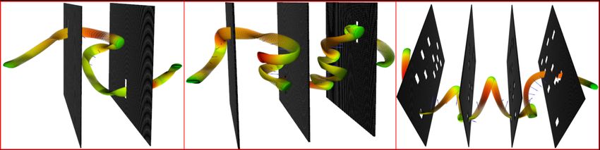

2 IEEE ROBOTICS AND AUTOMATION LETTERS. PREPRINT VERSION. ACCEPTED FEBRUARY 2021

 II. Related Work the acceleration of center of mass and the angular velocity of
 Polynomial trajectory planning [6] jointly optimizes the a standard quadrotor in terms of the flat outputs are
pieces of a piecewise polynomial trajectory for flat systems x¥ = − z + z (1)
[13] in a numerically robust and unconstrained fashion. It is  2  1 0 0
 1 
 = − 1  = 0 1 0 R−1 ẍ
   
a sequential method that uses a piecewise linear path as a (2)
seed for polynomial trajectory generation. Consequently, they  3  0 0 0
    
do not handle attitude constraints for narrow gaps or perform where x is the position vector of the robot’s center of mass
global reasoning in case a part of the seed plan is invalid. in the inertial frame, is its mass, is the acceleration due
Several prior works have demonstrated aggressive maneuvers to gravity, R describes the rotation of the body frame with
for quadrotors that pass through narrow gaps [4], [5], [12] but, respect to the inertial frame , and are the angular
instead of solving the planning problem, those works focus on velocity vector and net thrust in the body-fixed coordinate
trajectory optimization with given attitude constraints. Those frame (Fig. 1). z is the unit vector aligned with the axis
constraints are often hand-picked beforehand or obtained using of the four rotors and indicates the direction of thrust, while
gap detection algorithms which only works for specific cases. −z is the unit vector expressing the direction of gravity.
 Aggressive quadrotor planning for large environments typ- The flatness property lets us calculate the quadrotor’s ori-
ically involves building a safe corridor [14] such as convex entation from the flat outputs and its derivatives. We make
decomposition of the free space [15], [16]. These methods a useful observation from Eq. 1 that the quadrotor can only
do not deal with attitude constraints and hence there is no accelerate in the direction of thrust and hence the attitude (roll
guarantee on planner’s completeness when the robot has to and pitch) is constrained given the thrust vector. This constraint
aggressively negotiate a narrow gap. Liu’s work [8], [17] on mapping is invertible and hence we can recover the direction
lattice search with predefined primitives for aggressive flight of acceleration from attitude. In Sec. V-A, we will describe
is the first method that attempts to incorporate quadrotor shape and explicitly derive how the magnitude of acceleration is
and dynamics in planning for large environments. It uses calculated by getting rid of the free variable in Eq. 1.
search-based methods to synthesize a plan over the lattice. Following [25], we use triple integrator dynamics with jerk
However, lattice search suffers from the curse of dimensionality input for quadrotor planning. Trajectory segments consisting
and their performance significantly depends on the choice of of three polynomial functions of time, each specifying the
discretization for the state and the action space. Barring the independent evolution of , , , is used for quadrotor planning
interplay of low and high-dimensional search, our work is between two states in the flat output space [26], [6], [25].
reminiscent of Theta* [18] as both the methods proceed by As the desired trajectory and its derivatives are sufficient to
rewiring each successor to the best ancestor possible. However, compute the states and control inputs in closed form, they
Theta* is a planning algorithm designed specifically for 2D serve as a simulation of the robot’s motion in the absence
and 3D grid search and not applicable to higher dimensional of disturbances. This powerful capability is enabled by differ-
planning like ours. ential flatness that eliminates the need for iterated numerical
 Sampling-based robot motion planning has a rich history integration of equations of motion, or a search over the space
owing to their simplicity and scalability to higher dimensions of inputs during each iteration of the planning algorithm.
[19], [20]. But for kinodynamic planning, they rely on the
“steer” operator which is often not efficient to compute [7]. IV. Problem Statement
They also suffer from the narrow passage problem [21],
 Let denote the translational variables of the quadrotor
take longer time to converge to a good quality path and
 including its position, velocity, acceleration and jerk, =
have unreliable intermediate path quality [20]. Despite that,
 [xT , ẋT , ẍT , ẍT ] T ∈ R12 . The 3D pose of the quadrotor is given
sampling-based trajectory optimization methods like LQR trees
 by the position of its center of mass x = [ , , ] T and orienta-
[9] with very high convergence time have enjoyed success
 tion (in Euler angles) = [ , , ] T in the inertial frame.
and even been applied to hybrid systems [22]. These methods
 Given (a) an initial state s0 = [ T 0 , 0 T , ( 0 ) T , ( 0 ) T ] T
focus on the conditions for guaranteed execution based on the
 where and are the angular velocity and angular accel-
geometry of the trajectory funnels and the obstacles and even
 eration of the body frame , (b) a goal region X , (c) the
demonstrate it on a spherical quadrotor [23]. However, deriving
 planning space X with the obstacles X , the task is to find
such relations become extremely hard or almost impossible if
 an optimal trajectory ∗ ( ) = [x∗ ( ) T , ẋ∗ ( ) T , ẍ∗ ( ) T , ẍ∗ ( ) T ] T
the quadrotor is approximated as an ellipsoid.
 according to Eq. 3, where x∗ ( ) ∈ X \ X , ∈ [0, ] or the
 corresponding control inputs u∗ ( ), ∈ [0, ]. X represents
III. Differential Flatness and Control of a Quadrotor all the configurations of the robot that are in collision (Sec.
 The quadrotor dynamics with four inputs (net thrust and the V-D2) with its shape taken into consideration.
body moment about each axis) is differentially flat [24]. In For aggressive flight, the dynamical constraints of the
other words, the states and inputs can be written as algebraic quadrotor in terms of thrust and torques that can be supplied
functions of the so-called flat outputs, , , , and (yaw) by the motors have to be satisfied while planning. Using
and their derivatives. However, since the yaw is decoupled and the differential flatness property, these control saturation can
does not affect the system dynamics, we do not consider it be converted to componentwise box constraints on velocity,
during planning. The Newton’s equation of motion governing acceleration and jerk on each axis independently [27] as

NATARAJAN et al.: INTERLEAVING GRAPH SEARCH AND TRAJECTORY OPTIMIZATION FOR AGGRESSIVE QUADROTOR FLIGHT 3

| ẋ( )|  ẋ , | ẍ( )|  ẍ , |ẍ( )|  ẍ . Thus the time- where x¥ and z are the axis-wise components of acceleration
optimal path-planning for aggressive quadrotor flight can be and thrust vector. Rearranging the terms in Eq. 4 provides a
cast as the following optimization problem: linear constraint on acceleration independent of the thrust
 ∫ −z 
 z 
 0  x¥   0 
 min = kẍ( ) k 2 +  
 −z 0 z   ¥  =  z 
  x (5)
 
 
 x( ),u( ) , 0    
  0 −z z   ¥
 x   z 
 s.t. ẋ = (x, u),     
 |{z}
 
 | {z }
 x(0) = x0 , (3) W d
 W¥x = d (6)
 x( ) ∈ X ,
 We incorporate the constraint derived above in the joint
 | ẋ( )|  ẋ , | ẍ( )|  ẍ , |ẍ( )|  ẍ polynomial optimization method introduced in [6] to find a
 x( ) ∈ X \ X , u ∈ U ∀ ∈ [0, ] sequence of polynomials through a set of desired attitude
where and U denote the quadrotor dynamics and the set of all constrained waypoints. Thus, the first term of the cost function
attainable control vectors, is total cost of the trajectory in Eq. 3 can be transformed into product of coefficients of 
and is the penalty to prioritize control effort over execution polynomials and their Hessian with respect to coefficients
time . It is sufficient to find the optimal trajectory purely in per polynomial thereby forming a quadratic program (QP)
 ∫ 
terms of translational variables as the reminder of state can be
recovered using the results of differential flatness. = kẍ( ) k 2 = pT Hp (7)
 0
 where p∈ R represents all the polynomial coefficients
 V. Motion Planning For Aggressive Flight grouped together and H is the block Hessian matrix with
 Our trajectory planning framework consists of two overlap- each block corresponding to a single polynomial. Note that
ping modules: a grid-based graph search planner and a trajec- the integrand encodes the sequence of polynomial segments as
tory optimization routine. These two methods are interleaved opposed to just one polynomial and each block of the Hessian
to combine the benefits of former’s ability to search non- matrix is a function of time length of the polynomial segment.
convex spaces and solve combinatorial parts of the problem We omit the details for brevity and defer the reader to [6]
and the latter’s ability to obtain a locally optimal solution for a comprehensive treatment. Following [6], the requirement
not constrained to the discretized search space. We provide to satisfy the position constraints and derivative continuity is
analysis (Sec. V-C) and experimental evidence (Sec. VI) that achieved by observing that the derivatives of the trajectory
interleaving provides a superior alternative in terms of quality are also polynomials whose coefficients depend linearly on the
of the solution and behavior of the planner than the naive coefficients of the original trajectory. In our case, in addition to
option of running them in sequence [6]. position and continuity constraints we have to take the attitude
 We begin by providing a brief overview of the polynomial constraints into account via acceleration using Eq. 6.
 x¤   
trajectory optimization setup. This will be followed by the b
 =⇒ p = A−1 c
  
 Ap = x¥  =⇒ Ap =
   (8)
description of the INSAT framework and how it utilizes graph
 ẍ W−1 d
search and polynomial trajectory generation. We then analyse   | {z }
INSAT’s guarantees on completeness. c
 where the matrix A maps the coefficients of the polynomials
 to their endpoint derivatives and b contains all other derivative
A. Attitude Constrained Joint Polynomial Optimization values except acceleration which is obtained using Eq. 6. Using
 To generate a minimum-jerk and minimum-time trajectory, Eq. 8 in Eq. 7
the polynomial generator should compute a thrice differentiable = cT A− T HA−1 c (9)
trajectory that guides the quadrotor from an initial state to Note that due to the interdependent acceleration constraint
a partially defined final state by respecting the spatial and (Eq. 5) imposed at the polynomial endpoints, we lost the
dynamic constraints while minimizing the cost function given ability to solve the optimization independently for each axis.
in Eq. 3. For quadrotors, it is a common practice to con- Nevertheless, the key to the efficiency of our approach lies in
sider triple integrator dynamics and decouple the trajectory the fact that solving a QP like Eq. 7 subject to linear constraints
generation [25], [8] into three independent problems along in Eq. 8 or in their unconstrained format in Eq. 9 is incredibly
each axis. However, for attitude constrained flight, although fast and robust to numerical instability. Thus the total jerk and
the dynamic inversion provided by the flatness property aids time cost to be minimized becomes
in determining the direction of acceleration from the desired 
 ∑︁
attitude, the corresponding magnitude cannot be computed by = cT A− T HA−1 c + (10)
 | {z }
axis independent polynomial optimization. We note from Eq. =1
 | {z }
1 that the thrust supplied by the motors is a free variable 
which can be eliminated to deduce a constraint relationship where expresses the time length of the th polynomial. As
between the components of the acceleration vector x¥ and the mentioned before, the Hessian depends on the choice of time
direction of thrust in body frame z as follows length of the polynomial segment and hence the overall cost is
 x¥ x¥ x¥ − minimized by running a gradient descent on and evaluating
 
 = = (4)
 z z z corresponding to a particular .

4 IEEE ROBOTICS AND AUTOMATION LETTERS. PREPRINT VERSION. ACCEPTED FEBRUARY 2021

B. INSAT: Interleaving Search And Trajectory Optimization Algorithm 1 INSAT
 1: procedure Key(s )
 To plan a trajectory that respects system dynamics and 2: return (s ) + ∗ ℎ(s )
controller saturation, and simultaneously reason globally over
 3: procedure GenerateTrajectory(s , n )
large non-convex environments, it is imperative to maintain the
 z = [ (n ), − (n ) (n ), (n ) (n )] >
 
 4:
combinatorial graph search tractable. To this end, we consider ¥
 x −1
 T 5: n = W d ⊲ Differential flatness Eq. 5
a low-dimensional space X (5D) comprising {x , , }. The
 c = [(s T
 ) , (n ) T , (s ) T ] T ⊲ Eq. 8
discrete graph search runs in X which typically contains 6: 
variables of the state whose domain is non-convex. It then 7: n ( ) = Ó (c) ⊲ Eq. 10
seeds the trajectory optimization, such as the one in Sec. V-A, 8: if n ( n ). () ⊲ Sec. V-D2
in the high-dimensional space X (12D) comprising {xT , ẋT , n ( n ). () then ⊲ Sec. V-D1
ẍT , ẍT }, to in turn obtain a better estimate of the cost-to-come 9: return n ( )
value of a particular state for the graph search. The subscripts 10: else
 and refer to the low and high-dimensional states. 11: for m ∈ (s ( )) do
 
 Alg. 1 presents the pseudocode of INSAT. Let s ∈ X 12: c = [(m ) T , (n ) T , (s ) T ] T ⊲ Eq. 8
and s ∈ X be the low-dimensional and high-dimensional 13: r ( ) = (c) ⊲ Eq. 10
 Ó
state. The algorithm takes as input the high-dimensional start 14: if r ( n ). () ⊲ Sec. V-D2
and goal states s 
 , s and recovers their low-dimensional r ( n ). () then ⊲ Sec. V-D1
 
 15: n ( ) = (m ( ), r ( ))
counterparts s , s (lines 20-22). The low-dimensional
 16: (n ( ))
free space X \ X is discretized to build a graph G to
 17: return n ( )
search. To search in G , we use weighted A* (WA*)[28] which
 18: return Tunnel traj. w/ discrete ∞ cost ⊲ Sec. V-C
maintains a priority queue called OPEN that dictates the order 
of expansion of the states and the termination condition based 19: procedure Main(s , s )
 
on Key(s ) value (lines 1, 25). Alg. 1 maintains two functions: 20: (s 
 )
 x
 = (s )
 x
 ; (s ) x = (s ) x
 x¥
cost-to-come (s ) and a heuristic ℎ(s ). (s ) is the cost of 21: (s )
 , 
 = Obtain from (s ) ⊲ Eq. 1
 (s ) , = Obtain from (s ) x¥
 
the current path from the start state to s and ℎ(s ) is an 22: ⊲ Eq. 1
underestimate of the cost of reaching the goal from s . WA* 23: ∀s , (s ) = ∞; (s 
 
 ) = 0
initializes OPEN with s 
 
 (line 24) and keeps track of the 24: Insert s 
 
 in OPEN with Key(s 
 
 )
 
expanded states using another list called CLOSED (line 29). 25: while Key(s ) < ∞ do
 A graphical illustration of the algorithm is provided in Fig. 26: s = OPEN. ()
2. Each time the search expands a state s , it removes s from 27: for s0 ∈ (s ) do
OPEN and generates the successors as per the discretization 28: n = (s0 )
(lines 26-28). For every low-dimensional successor n , we 29: if n ∈ CLOSED then
solve a trajectory optimization problem described in Sec. V-A 30: n = (s0 ); (n ) = ∞ ⊲ Sec. V-C
to find a corresponding high-dimensional trajectory from start 31: n ( ) = GenerateTrajectory(s Ó , n )
to goal via n (lines 6-7, Fig 2). Note that the trajectory op- 32: if n ( ). () ⊲ Sec. V-D2
timization is performed in the space of translational variables n ( ). () then ⊲ Sec. V-D1
 
but n specifies an attitude requirement. So prior to trajectory 33: ( ) = (n ( )) ⊲ Eq. 3
optimization, we utilize the differential flatness property to 
 34: Insert/Update n in OPEN with Key( )
transform the attitude of the quadrotor to an instantaneous 35: if (n ( n )) < (n ) then ⊲ Eq. 3
 ¥
direction and magnitude of acceleration nx to be satisfied (line 36: (n ) = (n ( n )) ⊲ Eq. 3
5, Eq. 5). The trajectory optimization output n ( ) is checked 37: Insert/Update n in OPEN with Key(n )
for collision and control input feasibility (line 8, Sec. V-D). If
the optimized trajectory n ( ) is in collision or infeasible (Fig. all the waypoint and derivative constraints (Fig. 2-Right)
2-Left), the algorithm enters the repair phase (lines 10-17). until convergence or trajectory becoming infeasible, whichever
 The repair phase is same as the first call to the optimizer occurs first. We remark that, within GenerateTrajectory(),
except that instead of the start state s 
 
 , we iterate over the the trajectory is checked for collision and feasibility only until
waypoints m (line 11) of the parent state’s trajectory s ( ) the waypoint n indicated by time n (lines 8, 14) although
in order (lines 11-14, Fig. 2-Center). It has to be noted that the trajectory connects all the way from start to goal via n .
the computational complexity of trajectory optimization QP is The validity of the full trajectory is checked in Main() (line
same for both the initial attempt and the repair phase as the 32) to be considered as a potential goal candidate (line 32-34).
sequence of polynomials from s 
 
 to m is unmodified.
Upon finding the state m which enables a high-dimensional C. Completeness Analysis of INSAT
feasible trajectory from start to goal via n , the full trajectory We import the notations X , G from V-B. G =
n ( ) is constructed by concatenating m ( ) up to m and (V , E ) where V and E are set of vertices and edges,
 
the newly repaired trajectory, r ( ), starting from m (line X = X \ X , G be any path in G , ( ) be the
15). The final trajectory is obtained by warm starting the low-dimensional trajectory and ( ) be the high-dimensional
optimization with the trajectory n ( ) as the seed and relaxing trajectory that is snap continuous.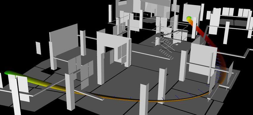

NATARAJAN et al.: INTERLEAVING GRAPH SEARCH AND TRAJECTORY OPTIMIZATION FOR AGGRESSIVE QUADROTOR FLIGHT 5

Fig. 2: Graphical illustration of the GenerateTrajectory() function of INSAT (Alg 1). Here the state s is expanded and a trajectory is
optimized for its successor n . LEFT: At first, the optimizer tries to find a trajectory directly from start to goal via n (n ’s high-dimensional
counterpart) as shown in red (lines 6-7). CENTER: If the portion of the trajectory from the first attempt up to n is input infeasible or
in collision (as in LEFT), then instead of the start state the earliest possible waypoint m (m ’s high-dimensional counterpart) on the
high-dimensional trajectory s ( ) is selected and a new trajectory segment is incrementally optimized (shown in red) as in lines 11-14.
RIGHT: Once a set of collision free and feasible trajectory segments are found, we refine the trajectory by relaxing all the waypoint and
derivative constraints (convergence shown with different shades of red). Note that this stage can consist of several polynomials being jointly
optimized, however, the convergence is extremely fast due to warm starting (line 16).
 
 Assumption (AS): If there exists ( ) ∈ X then there 18). The tunnel trajectory between m and n +1 (i) is collision-
exists a corresponding path G in G free under AS (ii) satisfies the boundary pose and derivative
 constraints (iii) snap continuous. The existence of such a tunnel
 G = {( , 0) | , 0 ∈ V , ( , 0) ∈ E , T ( , 0) ⊆ X 
 
 }
 trajectory can be shown using trigonometric bases but it is
where T ( , 0) is the tunnel around the edge ( , 0) (Fig. 3). beyond the scope of this proof. The “base case” of G , = 0
 
Theorem 1. ∃ ( ) ∈
 
 X =⇒ ∃ ( ) ∈
 
 X with 1 node (s 
 
 ) is collision-free s 
 
 ( ) ∈ X . And
 
 INSAT finds ( ) ∈ X 
 +1 even at ( + 1)th step. Hence,
Proof. Using quadrotor’s differential flatness all the variables INSAT is a provably complete algorithm. 
of X can be recovered from the variables in X . So the map
 
M : X ↦→ X is a surjection. But X = {x ∈ X |
 ( ) D. Trajectory Feasibility
M (x ) ∈ X } and hence the map M 
 : X ↦→
 To plan for aggressive trajectories in cluttered environments,
X is also a surjection. 
 we approximate the shape of the quadrotor as an ellipsoid to
 
Theorem 2 (Completeness). If ∃ ( ) ∈ X , then INSAT capture attitude constraints and check for collision. During a
is guaranteed to find a 0 ( ) ∈ X . state expansion, once the high-dimensional polynomial trajec-
 
 tory is found from the start to goal via a successor, it is checked
 for any violation of dynamics and control input (thrust and
 angular velocity) limits.
 1) Input Feasibility: We use a recursive strategy introduced
 in [27] to check jerk input trajectories for input feasibility
 by binary searching and focusing only on the parts of the
 polynomial that violate the input limits. The two control inputs
 to the system are thrust and the body rate in the body frame.
 For checking thrust feasibility, the maximum thrust along each
Fig. 3: Part of the high-dimensional trajectory n ( ) from s 
 
 to
 axis is calculated independently from acceleration (Eq. 1), by
 
s via the expanded node m and its successor n . The portion performing root-finding on the derivative of the jerk input
of n ( ) between m and n is guaranteed to lie within the tunnel polynomial trajectory. The maximum/minimum value among
(yellow) formed by m and n and is called as tunnel trajectory.
 all the axes is used to check if it lies within the thrust limits.
 For body rate, its magnitude can be bounded as a function of
Proof. Inference (IN): If AS holds, it is enough to search G 
 the jerk and thrust (Eq. 2). Using this relation, we calculate the
instead of X . Then from Theorem. 1 we can deduce that
 body rate along the trajectory and check if it entirely lies within
there exists a G in G if ∃ ( ) ∈ X . the angular velocity limits. Note that, in the implementation,
 Thus to prove the completeness of INSAT, we have to show these two feasibility tests are done in parallel.
that Alg. 1 finds a 0 ( ) ∈ X 
 
 for any G in G (i.e 2) Collision Checking: We employ a two level hierarchical
converse of IN). We prove by induction. At th step of INSAT, collision checking scheme. The first level checks for a conser-
let G = (V , E ) be the low-dimensional graph for which vative validity of the configuration and refines for an accurate
 
there exists a ( ) ∈ X from s 
 
 to any s ∈ V . collision check only if the first level fails. In the first level, we
The induction is to prove that, at ( + 1)th step, after adding approximate the robot as a sphere and inflate the occupied cells
any number of nodes to get G +1 = (V +1 , E +1 ), INSAT is of the voxel grid with its radius. This lets us treat the robot as a
 
guaranteed to find +1 ( ) ∈ X from s 
 
 ∈
 to every s +1 single cell and check for collision in cells along the trajectory.
V +1 . Let m ∈ V be the node expanded at ( +1)th step from The second level follows the ellipsoid based collision checking
G to generate a successor n +1 ∈ V and the graph G . We
 +1 +1
 that takes the actual orientation of the quadrotor into account
 
know that m ( ) ∈ X . So even if the basic (lines 6-9) and
 [8]. By storing the points of the obstacle pointcloud in a KD-
the repair (lines 10-17) phases fail (Sec. V-B), Alg. 1 falls back tree, we are able to crop a subset of the points and efficiently
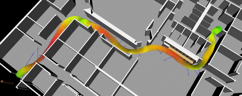
to finding the tunnel trajectory to concatenate with m ( ) (line check for collisions only in the neighborhood of the robot.

6 IEEE ROBOTICS AND AUTOMATION LETTERS. PREPRINT VERSION. ACCEPTED FEBRUARY 2021

 (a) Side views. LEFT: #Walls: 2, #Holes/wall: 1. CENTER: #Walls: 3, #Holes/wall: 1. RIGHT: #Walls: 4, #Holes/wall: 11

 (b) L&R side views. LEFT: #Walls: 2, #Holes/wall: 11. CENTER: #Walls: 3, #Holes/wall: 11. RIGHT: Velocity magnitude
Fig. 4: Visualization of trajectory planned by the proposed method in the walls and windows environment. The environment consists of
parallel walls with narrow holes (windows) smaller than the size of the quadrotor. The trajectory is represented as a sequence of ellipsoid
which approximates the quadrotor’s shape to plan in attitude constrained environments. The color gradient from green to red expresses the
magnitude of instantaneous velocity while the arrows along the trajectory denote the magnitude and direction of acceleration. The dynamically
stable agile behavior of the planner is analyzed in Sec. VI-A.
 #Windows Planning Time (s) Success Rate (%) Solution Cost (×105 ) Execution Time (s)
 #Walls Wall gap (m)
 per wall INSAT Base A INSAT Base A INSAT Base A INSAT Base A
 5 19.37 ± 17.34 122.5 ± 88.44 100 36 3.7 7.18 9.12 ± 1.04 10.4 ± 1.18
 1
 9 29.76 ± 28.41 180.47 ± 93.22 100 24 5.5 7.48 9.42 ± 1.54 10.81 ± 1.71
 5 46.58 ± 49.76 97.15 ± 70.01 100 100 6 6.16 6.93 ± 1.89 8.97 ± 2.25
 2 5
 9 22.07 ± 38.89 77.64 ± 58.8 100 100 5.5 6.9 8.88 ± 2 9.49 ± 2.58
 5 19.13 ± 21.81 66.62 ± 56.51 100 100 4.21 6.9 9.45 ± 1.42 9.19 ± 2.53
 10
 9 30.56 ± 24.08 60.81 ± 43.66 100 100 4.3 6.14 6.87 ± 1.62 8.45 ± 1.69
 1 5 83.33 ± 68.54 112.33 ± 87.24 100 24 8.69 9.38 11.5 ± 3.21 13.7 ± 2.74
 3 5 5 62 ± 80.97 224.60 ± 309.67 100 100 8 7.3 9.88 ± 1.66 10.8 ± 2.91
 10 5 18.7 ± 18.9 59.76 ± 56.73 100 100 5.01 6.99 8.83 ± 1.84 9.84 ± 2.15
 Planning Time (s) Success Rate (%) Solution Cost (×105 ) Execution Time (s)
 Map
 INSAT Base-A Base-B INSAT Base-A Base-B INSAT Base-A Base-B INSAT Base-A Base-B
 Willow Garage (2.5D) 40.05 ± 77.09 18.73 ± 46.7 2.55 ± 1.18 100 100 6 3.33 ± 4.92 3.73 ± 2.54 4.34 ± 1.1 14.5 ± 6.14 7.78 ± 5.33 2.54 ± 2
 Willow Garage (3D) 57.64 ± 97.24 89.8 ± 88.31 6.53 ± 2.49 100 100 10 5 ± 5.27 1.56 ± 0.91 7.38 ± 2.67 10.11 ± 6.8 3.21 ± 1.4 4.5 ± 1.78
 MIT Stata Center (3D) 5 ± 7.18 83.2 ± 91.94 3.94 ± 1.2 100 14 32 6.68 ± 7.65 3.44 ± 2.33 2.24 ± 0.88 7.12 ± 3.44 5.7 ± 3.34 7.7 ± 2.93

TABLE I: Comparison of INSAT with search-based planning for aggressive SE(3) flight (Base-A) [8] and polynomial trajectory planning
(Base-B) [6]. The top table displays the average and standard deviation of the results for walls and windows environment and the bottom
table for indoor office environment. Note that INSAT consistently outperforms the baselines across different types of environments.
 VI. Experiments and Results polynomial trajectory planning (Base-B) [6]. We used the
 We evaluate the empirical performance of INSAT in sim- AscTec Hummingbird quadrotor [30] in the Gazebo simulator
ulation against two baselines in two types of environments: [31] as our testing platform. All the methods are implemented
1) a walls and windows environment that mimics an array of in C++ on a 3.6GHz Intel Xeon machine.
narrowly spaced buildings each containing several windows
smaller than the radius of the quadrotor and 2) a cluttered A. Walls and Windows Environment
indoor office environment, namely Willow Garage and MIT For the walls and windows environment, we randomly
Stata Center [29] maps. Together the environments convey a generated several scenarios with arbitrary number of parallel
story of a quadrotor aggressively flying through several tall walls where each wall contains random number of windows
raised office buildings. The baseline methods include search- (gaps smaller than quadrotor’s radius). The goal of the planner
based planning for aggressive SE(3) flight (Base-A) [8] and is to generate a trajectory to fly from one end of the parallel

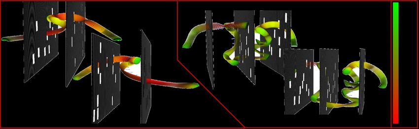
NATARAJAN et al.: INTERLEAVING GRAPH SEARCH AND TRAJECTORY OPTIMIZATION FOR AGGRESSIVE QUADROTOR FLIGHT 7

 B. Indoor Office Environment
 We also tested INSAT on the same maps and planning
 dimensions reported in the baseline papers i.e maps of Willow
 Garage (2.5D [8] and 3D) and MIT Stata Center (3D) [6].
 These are large, cluttered, office environments that contain a
 number of narrow gaps smaller than the size of quadrotor. The
 final trajectory from one example is shown in Fig. 5 and the
 statistics are provided in the bottom half of Table. I. Willow
 Garage map has tight spaces and high obstacle density but
 (a) Willow Garage office environment
 uniform obstacle distribution along its height compared to the
 MIT map that has scattered obstacles with varying distribution.
 Thus, Base-B performs well only in the MIT map as it does
 not necessitate attitude constrained planning.
 From the bottom half of Table I we see that INSAT has
 the highest success rate. For the baselines, we used the same
 parameters supplied by the authors. In 2.5D planning, Base-
 A is faster than INSAT as it has a low branching factor
 with precomputed motion primitives. However, this difference
 vanishes in 3D because of exponential complexity with longer
 times spent to escape local minimas in Base-A and relatively
 (b) MIT Stata Center
 faster speeds of polynomial trajectory generation in INSAT.
Fig. 5: INSAT in indoor office environments in 3D mode. The parameters that determine INSAT’s performance including
Trajectories are expressed in the same format as Fig. 4 planning time, continuity and obeying dynamic constraints are:
walls to the other by negotiating the windows and satisfying x ẋ ẍ ẍ 
their corresponding attitude constraints. Note that the planner 0.2m 0.1rad 10m/s 20 / 2 50 / 3 500 10N 0.05s
also has to figure out the right topology for the solution, i.e., the
 where x and d are the linear and angular discretization
sequence of windows it can fly through to get to its goal. For
 used for low-dimensional search, is the maximum thrust,
this environment, we compared only against Base-A [8] as the
 is the time step used for collision checking and is the
other baseline (Base-B) [6] does not explicitly handle attitude
 penalty to prioritize control effort over execution time. The
constraints needed to plan in these scenarios and therefore had
 execution and trackability of the generated trajectories are
a very low success rate.
 evaluated in Gazebo simulator 1. One critical parameter is
 The planned trajectory from INSAT is visualized (Fig. the resolution of the low-dimensional grid that guarantees the
4) as a sequence of ellipsoids approximating the shape of planner’s completeness (refer Sec. V-C).
quadrotor to handle SE(3) constraints. We evaluated INSAT
and Base-A over 50 random start and goal states in each of C. INSAT vs Sequential (S) vs Lattice Search (L) methods
the different environment scenarios (top half of Table I). For S methods [6] like Base-A first search for a path ignoring the
the heuristic, we computed 3D (x, y, z) distances to the goal dynamics and then refine to find the feasible trajectory using
while accounting for obstacles and assuming a point robot. To trajectory optimization. L methods [8] like Base-B discretize
compute it, we ran a single 3D Dijkstra’s search backwards the entire full-dimensional space and precompute the lattice
from the goal to obtain distances for all the cells. The results with motion primitives offline. INSAT finds plans with superior
show that INSAT consistently outperforms Base-A in terms of behavior compared to S and L because:
the trajectory computation time and execution time. All the Computational Complexity: L methods have fundamental
methods are timed out after 300s. The success rate shows that limitation as their performance significantly depends on the
INSAT finds a solution in every scenario as opposed to Base- choice of discretization for the state and action space, the
A’s varying levels of reliability. Specifically, we see that the primitive length along which the control input is constant
Base-A struggles when the number of windows per wall is and the lattice density itself [32]. Additionally, solving the
decreased making the planner vary altitude and find a window boundary value problem to generate primitives that connect
at different height to get through. This is because Base-A is the discrete cell centers can be difficult or impossible [32].
 
a lattice search method whose performance strongly depends In our method, albeit X is discretized, there is no such
on parameters such as the density and the length of primitives 
 discretization in X , where we let the optimization figure
in the lattice. While reproducing the results in their paper [8], out the continuous trajectory that minimizes the cost function
we found that their planner used a 2.5D lattice (primitives are (Eq. 3). As S methods decouple planning in X and X ,
restricted to a single plane). Our scenario requires planning they cannot handle attitude constraints and is restricted to a
in 3D with varying altitude. Despite tuning the parameters to path found in X when planning in X . In S, replacing the
fit 3D configuration for Base-A, the exponential increase in entire trajectory found in X with tunnel trajectory (Fig. 3)
computation combined with the discretization introduced by
the lattice sacrificed their success rate. 1A movie of INSAT in Gazebo simulator is available here.

8 IEEE ROBOTICS AND AUTOMATION LETTERS. PREPRINT VERSION. ACCEPTED FEBRUARY 2021

can violate the limits of velocity or jerk. Note that INSAT [6] C. Richter, A. Bry, and N. Roy, “Polynomial trajectory planning for
actively tries to minimize such violations (lines 11-14). Thus, aggressive quadrotor flight in dense indoor environments,” in Robot.
 Research. Springer, 2016, pp. 649–666.
as substantiated by our experiments, interleaving these schemes [7] S. M. LaValle and J. J. Kuffner Jr, “Randomized kinodynamic planning,”
provide a superior alternative by minimizing the effect of dis- Int. J. Robot. Research, vol. 20, no. 5, pp. 378–400, 2001.
cretization and keeping the full dimensional search tractable. [8] S. Liu, K. Mohta, N. Atanasov, and V. Kumar, “Search-based motion
 planning for aggressive flight in se (3),” IEEE Robot. Autom. Lett., vol. 3,
 Energy Accumulation Maneuvers: In tight spaces, a no. 3, pp. 2439–2446, 2018.
quadrotor might have to perform a periodic swing or re- [9] R. Tedrake, I. R. Manchester, M. Tobenkin, and J. W. Roberts, “Lqr-
visit a state to accumulate energy and satisfy certain pose trees: Feedback motion planning via sums-of-squares verification,” Int.
 J. Robot. Research, vol. 29, no. 8, pp. 1038–1052, 2010.
constraints. So a high-dimensional trajectory solution might [10] E. A. Hansen and R. Zhou, “Anytime heuristic search,” J. Artificial
require revisiting a low-dimensional state with a different value Intelligence Research, vol. 28, pp. 267–297, 2007.
for the high-dimensional variables (i.e. same x but different [11] M. Likhachev, G. J. Gordon, and S. Thrun, “Ara*: Anytime a* with
 provable bounds on sub-optimality,” in Advances in neural information
x¤ or ẍ). This is handled by duplicating the low-dimensional processing systems, 2004, pp. 767–774.
state if it is already expanded (lines 29-30). S methods cannot [12] G. Loianno, C. Brunner, G. McGrath, and V. Kumar, “Estimation,
handle this case as they decouple planning in X and X . control, and planning for aggressive flight with a small quadrotor with a
 single camera and imu,” IEEE Robot. Autom. Lett., pp. 404–411, 2016.
Consequently, observe in Fig. 4 that to negotiate a window [13] M. J. Van Nieuwstadt and R. M. Murray, “Real-time trajectory generation
in the wall, the quadrotor actively decides to fly in either for differentially flat systems,” Int. J. Robust Nonlinear Control: IFAC-
direction relative to the window to accumulate energy such Affiliated Journal, vol. 8, no. 11, pp. 995–1020, 1998.
 [14] S. Liu, M. Watterson, K. Mohta, K. Sun, S. Bhattacharya, C. J. Taylor,
that an attitude constraint via acceleration (Eq. 5) can be and V. Kumar, “Planning dynamically feasible trajectories for quadrotors
satisfied at the window. Another interesting behavior is the using safe flight corridors in 3-d complex environments,” IEEE Robot.
decision to fly down or rise up helically (Fig. 4a-CENTER Autom. Lett., vol. 2, no. 3, pp. 1688–1695, 2017.
 [15] R. Deits and R. Tedrake, “Efficient mixed-integer planning for uavs in
and Fig. 4b-CENTER) in between the tightly spaced walls cluttered environments,” in Proc. IEEE Int. Conf. Robot. Autom. IEEE,
in order to maintain stability or potentially avoid vortex ring 2015, pp. 42–49.
states and simultaneously not reduce the speed by taking slower [16] B. Landry, R. Deits, P. R. Florence, and R. Tedrake, “Aggressive
 quadrotor flight through cluttered environments using mixed integer
paths. Such a behavior leveraging the dynamic stability of the programming,” in Proc. IEEE Int. Conf. Robot. Autom. IEEE, 2016,
quadrotor along with the choice of windows to fly through pp. 1469–1475.
via global reasoning is a direct consequence of interleaving [17] S. Liu, N. Atanasov, K. Mohta, and V. Kumar, “Search-based motion
 planning for quadrotors using linear quadratic minimum time control,”
trajectory optimization with grid-based search. in Proc. IEEE/RSJ Int. Conf. Intell. Robots Syst., 2017, pp. 2872–2879.
 VII. Conclusion [18] K. Daniel, A. Nash, S. Koenig, and A. Felner, “Theta*: Any-angle path
 planning on grids,” J. Artificial Intelligence Research, vol. 39, 2010.
 We presented INSAT, a meta algorithmic framework that in- [19] L. E. Kavraki, P. Svestka, J.-C. Latombe, and M. H. Overmars, “Prob-
terleaves trajectory optimization with graph search to generate abilistic roadmaps for path planning in high-dimensional configuration
kinodynamically feasible trajectories for aggressive quadrotor spaces,” IEEE tran. on Robot. Autom., vol. 12, no. 4, pp. 566–580, 1996.
 [20] S. Karaman and E. Frazzoli, “Sampling-based algorithms for optimal
flight. We show that interleaving allows a flow of mutual infor- motion planning,” Int. J. Robot. Research, vol. 30, pp. 846–894, 2011.
mation and help leverage the simplicity and global reasoning [21] D. Hsu, L. E. Kavraki, J.-C. Latombe, R. Motwani, S. Sorkin, et al.,
benefits of heuristic search over non-convex obstacle spaces, “On finding narrow passages with probabilistic roadmap planners,” in
 Robotics: the algorithmic perspective: 1998 workshop on the algorithmic
and mitigate the bottleneck introduced by the number of search foundations of robotics, 1998, pp. 141–154.
dimensions and discretization using trajectory optimization. [22] S. Rajasekaran, R. Natarajan, and J. D. Taylor, “Towards planning and
 The trajectory generation method and graph search algo- control of hybrid systems with limit cycle using lqr trees,” in Proc.
rithm can be easily replaced with alternatives depending on IEEE/RSJ Int. Conf. Intell. Robots Syst. IEEE, 2017, pp. 5196–5203.
 [23] A. Majumdar and R. Tedrake, “Funnel libraries for real-time robust
the application. We also analysed the completeness property feedback motion planning,” Int. J. Robot. Research, pp. 947–982, 2017.
of the algorithm and demonstrated it on two very different [24] D. Mellinger and V. Kumar, “Minimum snap trajectory generation and
environments. Finally, we note that our method is not just control for quadrotors,” in Proc. IEEE Int. Conf. Robot. Autom., 2011,
 pp. 2520–2525.
limited to quadrotor planning and can be easily applied to [25] M. Hehn and R. D’Andrea, “Quadrocopter trajectory generation and
other systems like fixed-wing aircraft or mobile robots that control,” IFAC proceedings Volumes, vol. 44, pp. 1485–1491, 2011.
have differentially flat representations [33]. To the best of our [26] I. D. Cowling, O. A. Yakimenko, J. F. Whidborne, and A. K. Cooke,
 “Direct method based control system for an autonomous quadrotor,” J.
knowledge, INSAT is the first to interleave graph search with Intelligent & Robotic Systems, vol. 60, no. 2, pp. 285–316, 2010.
trajectory optimization for robot motion planning. [27] M. W. Mueller, M. Hehn, and R. D’Andrea, “A computationally efficient
 References motion primitive for quadrocopter trajectory generation,” IEEE Trans.
 Robot., vol. 31, no. 6, pp. 1294–1310, 2015.
 [1] M. Cutler and J. P. How, “Analysis and control of a variable-pitch [28] I. Pohl, “Heuristic search viewed as path finding in a graph,” Artificial
 quadrotor for agile flight,” J. Dyn. Sys., Meas., and Control, 2015. intelligence, vol. 1, no. 3-4, pp. 193–204, 1970.
 [2] D. Mellinger, N. Michael, and V. Kumar, “Trajectory generation and [29] M. Fallon, H. Johannsson, M. Kaess, and J. J. Leonard, “The mit stata
 control for precise aggressive maneuvers with quadrotors,” Int. J. Robot. center dataset,” Int. J. Robot. Research, vol. 32, pp. 1695–1699, 2013.
 Research, vol. 31, no. 5, pp. 664–674, 2012. [30] A. Technologies, “Ascending technologies, gmbh,” 2012.
 [3] M. Müller, S. Lupashin, and R. D’Andrea, “Quadrocopter ball juggling,” [31] N. Koenig and A. Howard, “Design and use paradigms for gazebo, an
 in Proc. IEEE/RSJ Int. Conf. Intell. Robots Syst. IEEE, 2011, p. 5113. open-source multi-robot simulator,” in 2004 Proc. IEEE/RSJ Int. Conf.
 [4] D. Falanga, E. Mueggler, M. Faessler, and D. Scaramuzza, “Aggressive Intell. Robots Syst., vol. 3, pp. 2149–2154.
 quadrotor flight through narrow gaps with onboard sensing and comput- [32] M. Pivtoraiko, I. A. Nesnas, and A. Kelly, “Autonomous robot navigation
 ing using active vision,” in Proc. IEEE Int. Conf. Robot. Autom. IEEE, using advanced motion primitives,” in IEEE Aerospace Conf., 2009, pp.
 2017, pp. 5774–5781. 1–7.
 [5] T. Hirata and M. Kumon, “Optimal path planning method with attitude [33] R. M. Murray, M. Rathinam, and W. Sluis, “Differential flatness of
 constraints for quadrotor helicopters,” in Proc. IEEE Int. Conf. Adv. mechanical control systems: A catalog of prototype systems.” Citeseer.
 Mechatronic Sys. IEEE, 2014, pp. 377–381.