Masking by Moving: Learning Distraction-Free Radar Odometry from Pose Information
←
→
Page content transcription
If your browser does not render page correctly, please read the page content below
Masking by Moving: Learning Distraction-Free
                                                Radar Odometry from Pose Information
                                                                     Dan Barnes, Rob Weston, Ingmar Posner
                                                                       Applied AI Lab, University of Oxford
                                                                  {dbarnes, robw, ingmar}@robots.ox.ac.uk

                                                  Abstract: This paper presents an end-to-end radar odometry system which deliv-
arXiv:1909.03752v4 [cs.CV] 17 Jan 2020

                                                  ers robust, real-time pose estimates based on a learned embedding space free of
                                                  sensing artefacts and distractor objects. The system deploys a fully differentiable,
                                                  correlation-based radar matching approach. This provides the same level of in-
                                                  terpretability as established scan-matching methods and allows for a principled
                                                  derivation of uncertainty estimates. The system is trained in a (self-)supervised
                                                  way using only previously obtained pose information as a training signal. Using
                                                  280km of urban driving data, we demonstrate that our approach outperforms the
                                                  previous state-of-the-art in radar odometry by reducing errors by up 68% whilst
                                                  running an order of magnitude faster.

                                                  Keywords: Perception, Radar, Odometry, Localisation, Deep Learning,
                                                  Autonomous Driving

                                         1   Introduction
                                         Robust ego-motion estimation and localisation are established cornerstones of autonomy. Emerging
                                         commercial needs as well as otherwise ambitious deployment scenarios require our robots to operate
                                         in ever more complex, unstructured environments and in conditions distinctly unfavourable for typ-
                                         ical go-to sensors such as vision and lidar. Our robots now need to see further, through fog, rain and
                                         snow, despite lens flare or when directly facing the sun. Radar holds the promise of remedying many
                                         of these shortcomings. However, it is also a notoriously challenging sensing modality: radar appli-
                                         cations are typically blighted by heterogeneous noise artefacts such as ghost objects, phase noise,
                                         speckle and saturation. In response, previous approaches to utilising radar for robot navigation have
                                         often tried to manually extract features from noise corrupted radar scans, commonly relying on
                                         simplifying assumptions on the distribution of power returns [1], manually designed heuristics [2],
                                         or features designed for different modalities [3, 4]. Nevertheless, the recent seminal work by Cen
                                         et al. [2] has firmly established radar as a feasible alternative to complement existing navigation
                                         approaches when it comes to ego-motion estimation.
                                         Beyond the basic methodology for pose estimation, the prevalence of vision- and lidar-based ap-
                                         proaches in this space has given rise to a number of useful methods beyond those currently utilised
                                         for radar. State-of-the-art visual odometry, for example, leverages learnt feature representations [5]
                                         as well as attention masks filtering out potentially distracting objects [6]. Lidar-based methods using
                                         correlative scan matching [7] typically achieve highly accurate and intuitively interpretable results.
                                         Inspired by this prior art, the aim of our work is to provide a robust radar odometry system which is
                                         largely unencumbered by either the typical radar artefacts or by the presence of potentially distract-
                                         ing objects. Our system is explicitly designed to provide robust, efficient and interpretable motion
                                         estimates. To achieve this we leverage a deep neural network to learn an essentially artefact and
                                         distraction free embedding space which is used to perform efficient correlative matching between
                                         consecutive radar scans. Our matching formulation is fully differentiable, allowing us to explicitly
                                         learn a representation suitable for accurate pose prediction. The correlative scan matching approach
                                         further allows our system to efficiently provide principled uncertainty estimates.
                                         Training our network on over 186,000 examples generated from 216km’s of driving, we outper-
                                         form the previous state of the art in challenging urban environments, reducing errors by over 68%
                                         and running an order of magnitude faster. Furthermore, our pose ground truth is gathered in a
                                         self-supervised manner, automatically optimising odometry, loop closure, and location constraints,
                                         enabling us to adapt to new locations and sensor configurations with no manual labelling effort.

                                         3rd Conference on Robot Learning (CoRL 2019), Osaka, Japan.
Z1                M1                   S1

                                                               ✓max ... ✓max
               Z2                M2                   S2

                                                                                                    p̄

                                                                                FFT Cross         Predict
    Radar Inputs      Predicted Masks      Feature Maps      Rotations of S1    Correlation   ?    Pose

Figure 1: Using masked correlative scan matching to find the optimum pose. Each radar scan is
passed to a CNN (pink) in order to generate a mask which is subsequently applied to the input radar
scan generating sensor artefact and distractor free representations S1 and S2 . We then calculate
the 2D correlation between S2 and rotated copies of S1 using the fft2d in order to generate the
correlation volume C. Finally we perform a softargmax operation in order to retrieve the predicted
pose. Crucially this pipeline is fully differentiable allowing us to learn the filter masks end to end.
A video summary of our approach can be found at: https://youtu.be/eG4Q-j3_6dk

2    Related Work

Compared to other sensing modalities such as vision or lidar, radar has received relatively little
attention in the context of robot navigation. Prior art in this area largely deploys a more traditional
processing pipeline consisting of separate feature extraction, data association and loss minimisation
steps, for example using the Iterative Closest Point (ICP) algorithm [8, 9]. For feature extraction
some works deploy approaches developed in vision, such as SIFT and SURF [3, 4], others more
bespoke methods such as CFAR filtering [10, 1], temporal-space continuity modelling [11, 12], and
grid-map features such as Binary Annular Statistics Descriptor (BASD) [13]. Most recently the
authors of [2] find point correspondences between point features extracted from raw scans using a
shape similarity metric. The final pose is then found by minimising the mean squared error between
point correspondences in close to real time.
By making use the Fourier transform correlation-based approaches are in contrast able to perform
a dense search over possible point correspondences [14] yielding intuitively interpretable results.
Similar approaches have also been applied successfully to lidar scan matching utilising efficient GPU
implementations [15] [7]. In comparison to ICP, correlation-based methods have been shown to be
significantly more robust to noise in pose initialisation [15]. While robustness and interpretability
are desirable, correlation-based methods operate on the assumption that the power returns from
a particular location are stationary over time so that a correlation operation produces meaningful
results. In reality, this is often not the case – for example when dynamic objects are present in the
scene. This problem is particularly pronounced in radar data due to the prevalence of noise artefacts.
Visual odometry systems, in contrast to radar-based ones, have a significant track record of suc-
cessful application in robotics and beyond. While traditional processing pipelines similar to the one
outlined for radar above have been widely deployed in this context (e.g. [16]) there has recently been
significant interest in moving away from separate processing steps towards end-to-end approaches.
Typically, a neural network is used to regress to a predicted pose directly from consecutive camera
images, learning the relationship between features and point correspondences in an integrated man-
ner (e.g. [5, 17]). In [18] the authors extend this approach by learning to predict the optimum pose
from stereo images alone. As in many related fields, these end-to-end approaches demonstrate the
potential for learning representations generally useful for odometry prediction. However, this comes
at the expense of entangling feature representation and data association, which makes the resulting
system significantly less interpretable. In contrast, the authors of [19] propose to learn a feature
embedding for localising online lidar sweeps into a previously known map, whilst maintaining the
interpretability, of a conventional correlative scan matching approach.
Due to the ubiquitous nature of vision-based systems researchers have also addressed challenges be-
yond the basic pose estimation task such as suppressing noise sources inherent in individual scenes.
For example, both [20] and [6] try to mask areas of an image where non-stationary features might
be found, which could corrupt the odometry estimate. Of particular relevance is [6], where a deep

                                                  2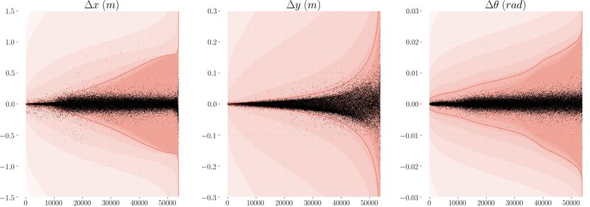
neural network is trained using data from other parts of the autonomous system in order to predict
human interpretable ephemerality masks indicating the presence of distractor objects in a scene.
Given the large body of evidence that end-to-end approaches tend to outperform more traditional,
hand-engineered processing pipelines it is tempting to conclude that our goal here is simply to de-
ploy a deep network to radar odometry. And we do indeed leverage deep learning in our system.
However, in doing so we are cognisant that we desire a system which ideally exploits the power of
representation learning offered by end-to-end approaches while at the same time leveraging the ef-
ficiency, robustness and interpretability offered by correlation-based methods. Thus, inspired by [6]
and similar to [19], we deploy a correlation-based matching method as part of an end-to-end system
which learns a radar embedding used to produce largely artefact and distraction-free representations
optimised for pose prediction. Both the masks obtained as well as the cost-volumes considered
remain as interpretable as more traditional approaches.

3     Deep Correlative Scan Matching with Learnt Feature Embeddings
Given two consecutive radar observations (Zt , Zt−1 ) we wish to determine the relative pose [R|t] ∈
SE(2) giving the transformation between the two co-ordinate systems at each time step. In achieving
this we aim to harness the efficiency, interpretability and robustness of correlative scan matching
assuming that the power returned from each world location is independent of the co-ordinate system
it was sensed in. In reality the power returns generated from real world scenes are far from stationary,
as dynamic objects move into and out of the field of view of the sensor and pertinent, random noise
artefacts obscure the true power returns, limiting the performance of an out-of-the-box correlative
scan matching system applied to radar data.
To address this, and inspired by the recent successes of learnt masking for pose prediction in vision
[6], we instead perform correlative scan matching over a learnt feature embedding, utilising a deep,
fully convolutional network to mask each radar scan as illustrated in Figure 1 (described in Sec-
tion 3.1). Through this approach we are able to harness the power of deep representation learning
whilst ensuring the feature representation remains interpretable through the geometrical constraints
imposed by the use of a correlative scan matching procedure. Crucially, we train our network by
supervising pose prediction directly. In doing so, our network naturally learns to attenuate distractor
objects such as moving vehicles and sensor noise as they degrade pose estimation accuracy, whilst
preserving features which are likely to be consistent between scans such as walls and buildings. This
leads to a 68% reduction in errors over the current state-of-the-art whilst, by making use of efficient
correlation computations using the Fast Fourier Transform (FFT), running an order of magnitude
faster.
Even in the limit of perfectly stationary power returns, uncertainty in our pose prediction still em-
anates from pathological solutions arising from the underlying scene topology. In Section 5.2 we
show how we are additionally able to quantify the uncertainty in our pose prediction, further aiding
the interpretability of our system.

3.1   Correlative Scan Matching with Learnt Feature Embeddings

Let (Zt−1 , Zt ) ∈ [0, 1]W ×H denote consecutive observations made by single sweeps of the radar
sensor, converted to Cartesian co-ordinates such that Ztu,v gives the power return at Cartesian co-
ordinate (x, y) at time t. Let p = [∆x, ∆y, ∆θ]T denote the parameters of the relative pose
[R|t] ∈ SE(2) between the co-ordinate frames at t − 1 and t. We aim to predict the optimum
pose from consecutive radar observations harnessing the efficiency, interpretability and robustness
of correlative scan matching,
                                     p̄ = arg max Zt ? Zt−1                                     (1)
                                             p∈SE(2)

where Zt ? Zt−1 is defined as the discrete cross correlation between Zt (after being warped by the
pose p) and Zt−1 .
In order to solve for the predicted pose p̄ we consider a brute force approach: we discretise our
search search space, calculating the cross correlation score for each pose on a regular grid of pose
candidates before utilising a soft-argmax operation to solve for the optimum pose to sub-grid reso-
lution accuracy. This is achieved efficiently using Algorithms 2 and 3. By utilising bi-linear inter-
polation for all re-size and rotation operations, and computing the cross-correlation using the highly
efficient 2D Fast Fourier Transform, we are able to search for the optimum pose over a large search
area, efficiently solving (1) whilst still maintaining end-to-end differentiability.

                                                   3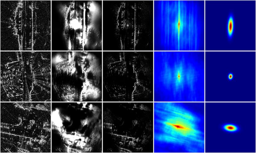
Central to this approach is an assumption that the power returned from each world location is in-
    dependent of the co-ordinate system it was sensed in. This assumption rarely holds in practice.
    Random noise artefacts, dynamic objects and changing scene occlusion cause fluctuations in the
    power field, degrading the accuracy of conventional correlation-based approaches applied to radar.
    To counter this, we propose to learn a feature representation S specifically optimised for correlative
    scan matching by filtering each radar scan S = M Z with a mask M = fα (Z) generated by
    a neural neural network fα (where denotes Hadamard product). By limiting each element of the
    mask to [0, 1] (using an element wise sigmoid), the network is able to learn to filter out distractor
    objects and noise in each sensor observation, before correlative scan matching is applied to find the
    optimum pose. By leveraging the differentiability of our approach for predicting p̄, we are able to use
    Algorithm 1, to learn a radar feature embedding specifically optimised for correlative scan matching
    by minimising the Mean Squared Error (MSE) over the training set, D = {(Zt , Zt−1 , p)n }N    n=1 ,

                                        α∗ = arg min Ep∼D ||p̄ − p||2

                                                                                                          (2)
                                                   α

    to update our network parameters α using conventional stochastic gradient descent based optimisers.

    3.2    Pose Uncertainty Estimation

    Pathological solutions arising from the underlying scene topology increase the uncertainty in our
    pose prediction even in the case of perfectly stationary power returns. In the real world identifying
    such cases is important in order to ensure robust operation. To this end, our approach also affords us
    a principled mechanism to estimate the uncertainty in each element of the predicted pose.
    In performing the soft-argmax operation, we first apply a temperature controlled softmax over the
    correlation scores for each candidate pose, to give weights ω = Softmax(βC), interpreted as the
    probability that each pose candidate is optimum. Assuming that our predicted pose is Gaussian
    distributed we can quantify the uncertainty in each pose prediction by using the weights ω to predict
    both the mean pose p̄ and the predicted co-variance Σ̄,
                            X                  X
                     p̄ =       ωs ps   Σ̄ =       ωs ps pTs − p̄p̄T   p(p|St ) ≈ N (p|p̄, Σ̄)            (3)
                            s                  s

    where we sum over all pose candidates. The softmax temperature parameter β plays an important
    role here: for high β our system is biased to the pose candidate with highest correlation and a low
    co-variance, whilst for low β to a weighted mean over a greater number of pose candidates and high
    co-variance.

    Algorithm 1: Training                                    Algorithm 2: Correlation
    Input:                                               1   function GetCorrelation(Gxyθ , X1 , X2 ) :
                                                         2      nx , ny , nθ ← Shape(Gxyθ )
    D // Dataset
    r // Search Region giving min and                    3      C = Zeros([nx , ny , nθ ])
        max range in ∆x, ∆y, ∆θ                          4      Gxy , Gθ ← Gxyθ
    δ // Grid resolution in each                         5      X1 , X2 ← Resize(X1 , X2 , Gxy )
        dimension δx , δy , δθ                           6      par for i ← 1 to nθ :
    β // Softmax Temperature Parameter                   7           X1R ← Rotate(X1 , Gθ [i])
     // Learning Rate                                   8           C[:, :, i] ←
    α // Initial Network Parameters                                   fft2d−1 fft2d(X1R ) fft2d(X2C )


1   Gxyθ = M eshGrid(r, δ)                               9      return C
2   while not converged do
3      Z1 , Z2 , p ← Sample(D)                               Algorithm 3: Soft Arg Max
                                                         1   function SoftArgMax(Gxyθ , C, β) :
4         M1 , M2 ← fα (Z1 ), fα (Z2 )                   2      ω ← Sof tmax(βC)
5         S1 , S2 ← M1 Z1 , M2 Z2                        3      Gx , Gy , Gθ ← Gxyθ
          C ← GetCorrelation(Gxyθ , S1 , S2 )
                                                                       P
6                                                        4      ∆x ← i,j,k ω Gx [i, j, k]
          p̄ ← Sof tArgM ax(Gxyθ , C, β)                               P
7                                                        5      ∆y ← i,j,k ω Gy [i, j, k]
       α ← α − ∇α L(p̄; p)
                                                                       P
8                                                        6      ∆θ → i,j,k ω Gθ [i, j, k]
9   end                                                  7      return[∆x, ∆y, ∆θ]

                                                             4
4 Experimental Setup
4.1 Dataset
To evaluate our approach we use the recently released Oxford Radar RobotCar Dataset [21], a radar
extension to the Oxford RobotCar Datsset [22], which provides Navtech CTS350-X radar data as
well as ground truth poses. The Navtech CTS350-X is a Frequency Modulated Continuous Wave
(FMCW) scanning radar without doppler information, configured to return 3768 power readings at a
resolution of 4.32cm across 400 azimuths at a frequency of 4Hz (corresponding to a maximum range
of 163m). The beam spread is 2 degrees in azimuth and 25 degrees in elevation with a cosec squared
beam pattern. We randomly split the traversals into training (80%) and evaluation (20%) partitions.
We additionally run spatial cross validation experiments, where each split occupies a different real
world region of the dataset. Further information on these results and the dataset can be found in the
appendix B.2, C.1.
To validate the advantages of learning masks directly from pose supervision we compare against
supervising the learnt masks directly on the proxy task of predicting temporally static occupied cells.
Training data for this is generated using a similar approach to [6]. For each radar scan we warp the
nearest radar sensor observation from each training traversal into the current pose before applying
a static power threshold. We then form a 2D histogram counting the number of thresholded power
returns that fall in each Cartesian grid cell. Any grid cell with more than 9 consistent observations
is assumed to be temporally stable and is labelled with a 1, whilst every other cell is set to 0. This is
repeated for every pose in every dataset. Examples of the masks generated by this approach can be
found in the appendix B.1.
4.2 Network Architecture and Training
In all experiments we use a U-Net style architecture [23] in which we encode the input tensor through
the repeated application of two convolutional layers (filter size 3x3) with ReLU activations before
a max pooling operation. After each max pool the width and height of the tensor are reduced by
a factor of 2 whilst the number of features is doubled, starting from 8 at the input to 256 at the
bottleneck of the network (corresponding to 5 max pools). The feature tensor is then converted
back to the original shape by the decoder through the application of bilinear upsampling followed
by two convolutional layers increasing the width and height and decreasing the feature channels by
a factor of 2. Skip connections at each level are implemented allowing information to flow from
encoder to decoder by stacking each representation with the output from the bilinear upsampling
layer in each case. The final convolutional layer has a single output channel with a sigmoid activa-
tion to limit the range to [0, 1]. We experiment with learning to mask both Cartesian and Polar radar
representations, as well as both single and dual configurations. In the dual case radar observations
are concatenated and passed as a single input producing two masks (instead of one) at the output.
An architecture diagram can be found in the appendix A.1. In all cases we consider a search re-
gion of [−50m, 50m] in ∆x and ∆y and [−π/12, π/12] in ∆θ. We experiment with the three grid
resolutions [0.2m, 0.4m, 0.8m] for δx and δy whilst fixing δθ to π/360.
Our network is implemented in Tensorflow [24] and trained using the Adam Optimiser [25] (learning
rate 1e − 5 and batch size 5) until the loss on a small validation set is a minimum. When training our
network with pose supervision we minimise the loss proposed in (2). We performed a grid search
over the optimum value of β and found setting it to 1 gave good performance.
4.3 Evaluation Metrics and Baselines
Our primary baseline is the current state of art for radar odometry [2] (implemented in C++) in which
the authors extract point features from consecutive radar scans before scan matching using a global
shape similarity score and refining by minimising mean squared error. Our radar was set to a range
resolution of 4.32cm, whilst the original algorithm was developed for a 17.28cm resolution. As such
we compare against [2] with full resolution radar scans and downsampled (with max pooling) to
17.28cm. For context we also provide visual odometry estimates (as in [2]). To assess the benefits
of learning feature masks specifically optimised for pose prediction, we benchmark against scan
matching on the raw radar scans without masking, as well as using the method proposed in [6] with
mask labels generated as described in Section 4.1. In this setup, we supervise (using a binary cross
entropy loss) the learnt masks directly (instead of supervising pose prediction). We also benchmark
against taking an off the shelf deep odometry model and training this for the task of radar pose
prediction. Specifically we use the UnDeepVO model proposed in [18].
5For all evaluations we follow the KITTI odometry benchmark [26]. For each 100m offset up to
800m, we calculate the average residual translational and angular error for every example in the
datastet normalising by the distance travelled. Finally, we average these values. Due to highly
skewed error distributions we report Inter Quartile Range (IQR) for each method instead of the
standard deviation. All timing statistics are calculated using a 2.7 GHz 12-Core Intel Xeon E5 CPU
and Nvidia Titan Xp GPU by averaging across 1000 predictions.
4.4 Uncertainty Evaluation
To assess the quality of the uncertainty predicted by our approach we observe that if our pose distri-
bution is Gaussian than the Mahalanobis error
d2 = (p − p̄)T Σ̄−1 (p − p̄), d2 ∼ χ2 (3) (4)
should be chi-squared distributed with degrees of freedom equal to the state dimensionality of p (in
this case three). As the mean of a chi-squared distribution is equal to the distributions
P degrees of
freedom, by averaging the mean Mahalanobis distance over the test dataset d¯2 = N1 n d2n we can
assess to what degree the uncertainties predicted by our approach are calibrated to the test errors [7].
Specifically, if d¯2
3 then our model is overly conservative in its predictions whilst if d¯2
3 it is
overly confident. In Section 5.2 we use this result to tune the temperature parameter β to provide us
with realistic uncertainties, that are calibrated to the true errors in our system.
5 Results
In this section we evaluate the performance of our approach. We find by utilising correlative scan
matching in combination with a learnt radar feature embedding we are able to significantly outper-
form the previous state of art in both prediction performance and speed. Additionally, we show
how, by tuning the temperature parameter of the softargmax, we are able to predict realistic and cal-
ibrated uncertainties, further increasing the interpretability of our system and allowing us to identify
pathological cases, crucial for robust operation in the real world.
Radar Input Predicted Mask Masked Features Correlation Covariance
Figure 2: Qualitative examples generated from our best performing model. Our network learns
to mask out noise and distractor objects whilst preserving temporally consistent features such as
walls, well suited for pose prediction. Predicted co-variance is high for pathological solutions aris-
ing through a lack of constraints in the x-direction (top), whilst stationary well-constrained scenes
result in low co-variance (middle). Motion blur increases the uncertainty due to ambiguous point
correspondence (bottom). Further examples can be found in Figure 8 in the appendix.
6Resolution Translational error (%) Rotational error (deg/m) Runtime (s)
Benchmarks (m/pixel) Mean IQR Mean IQR Mean Std.
RO Cen Full Resolution [2] 0.0432 8.4730 5.7873 0.0236 0.0181 0.3059 0.0218
RO Cen Equiv. Resolution [2] 0.1752 3.7168 3.4190 0.0095 0.0095 2.9036 0.5263
Raw Scan 0.2 8.3778 7.9921 0.0271 0.0274 0.0886 0.0006
Supervised Masks Polar 0.2 5.9285 5.6822 0.0194 0.0197 0.0593 0.0014
Supervised Masks Cart 0.2 5.4827 5.2725 0.0180 0.0186 0.0485 0.0013
Adapted Deep VO Cart [18] 0.2 4.7683 3.9256 0.0141 0.0128 0.0060 0.0003
Adapted Deep VO Polar [18] - 9.3228 8.3112 0.0293 0.0277 0.0093 0.0002
Visual Odometry [16] - 3.9802 2.2324 0.0102 0.0065 0.0062 0.0003
Ours
Polar 0.8 2.4960 2.1108 0.0068 0.0052 0.0222 0.0013
0.4 1.6486 1.3546 0.0044 0.0033 0.0294 0.0012
0.2 1.3634 1.1434 0.0036 0.0027 0.0593 0.0014
Cartesian 0.8 2.4044 2.0872 0.0065 0.0047 0.0113 0.0012
0.4 1.5893 1.3059 0.0044 0.0035 0.0169 0.0012
0.2 1.1721 0.9420 0.0031 0.0022 0.0485 0.0013
Dual Polar 0.8 2.5762 2.0686 0.0072 0.0055 0.0121 0.0003
0.4 2.1604 1.9600 0.0067 0.0053 0.0253 0.0006
0.2 1.2621 1.1075 0.0036 0.0029 0.0785 0.0007
Dual Cart 0.8 2.7008 2.2430 0.0076 0.0054 0.0088 0.0007
0.4 1.7979 1.4921 0.0047 0.0036 0.0194 0.0010
0.2 1.1627 0.9693 0.0030 0.0030 0.0747 0.0005
Table 1: Odometry estimation and timing results. Here “RO Cen” [2] is our primary benchmark
reported for 0.04m (full resolution) and, by downsampling, 0.17m (equivalent resolution for which
the approach was originally developed). For comparison we also provide performance results for
correlative scan matching on the raw power returns, for mask supervision (instead of supervising
the predicted pose directly), and adapting the deep VO network proposed in [18], alongside visual
odometry [16] for context. All baselines performed best at 0.2 m/pixel resolution where applicable
and the rest are omitted for clarity. We experiment with both polar and Cartesian network inputs at
multiple resolutions. Our approach outperforms the current state of the art, “RO Cen” (italics), for
all configurations of Cartesian / polar inputs and independent / dual masking at all resolutions. Our
best performing models in terms of speed and odometry performance are marked in bold.
5.1 Odometry Performance
Table 1 gives our prediction and timing results. We experiment with both Cartesian and Polar in-
puts to the masking network (converting the latter to Cartesian co-ordinates before correlative scan
matching), as well as experimenting with single and dual configurations as detailed in Section 4.2.
At all resolutions and configurations we beat the current state of the art with our best model reduc-
ing errors by 68% in both translation and rotation, whilst running over 4 times faster. Our fastest
performing model runs at over 100Hz whilst still reducing errors on the state of the art by 28% in
translational and 20% in rotational error (further results exploring the accuracy-speed trade off can
be found in A.2). We find that Cartesian network inputs typically outperform Polar (presumably
because correlative scan matching is performed in Cartesian space). Dual input configurations also
typically outperform passing single sensor observations to the masking network.
Key to our approach is learning a radar feature embedding that is optimised for pose prediction:
compared to correlative scan matching on the raw radar power returns this allows us to reduce
errors by over 85%. As predicted, optimising masks directly for pose prediction results in a higher
prediction accuracy than mask supervision labelling the temporally stationary scene directly. We
also find that simply adapting a deep odometry approach to radar results in significantly worse
performance. Our approach in contrast makes use of the inherent top down representation of a
radar observation which lends itself to a correlative scan matching procedure, whilst learning to
mask out noise artefacts which make pose prediction in radar uniquely challenging. In addition,
by adopting a correlative scan matching approach, our results remain interpretable: Figure 2 shows
several qualitative examples in which the network learns to mask noise artefacts and dynamic objects
in the scene whilst preserving features which are likely to be temporally stationary such as walls.
75.2 Uncertainty Prediction
In addition to the boosts in performance and speed afforded by our approach, we are also able to
estimate the uncertainty in each pose prediction: by interpreting the weights generated through the
temperature controlled softargmax operation as the probability that each pose candidate is optimum
we predict the co-variance Σ̄ in our prediction as detailed in Section 3.2.
We now use the methodology proposed in Section 4.4 to tune the temperature parameter β such
that the mean Mahalanobis distance d¯2 ≈ 3 producing uncertainties Σ̄ that are calibrated to the
errors in our system. Naively perturbing the temperature parameter away from its original value
β0 degrades pose prediction performance as the feature mask no longer corresponds to the β it was
optimised for. Instead, we calculate the predicted pose using β0 , whilst varying β to tune the co-
variance matrix. The results of this process (for the 0.8m resolution single mode Cartesian model
from Table 1) are shown in Figure 5.2 alongside the marginal distributions for the uncertainty in
each pose component plotted with the true errors in our system ordered by predicted uncertainty.
For a temperature parameter β = 2.789 the mean Mahalanobis distance d¯2 is equal to 2.99 giving us
well calibrated uncertainty predictions, whilst temperature parameters above and below this value
are overly certain and conservative respectively. There is a clear correlation between error and
uncertainty with most errors falling within the predicted uncertainty bounds.
Figure 2 shows Gaussian heat maps generated through our approach; the results are highly intu-
itive with feature embeddings well constrained in each dimension having smaller and symmetric
co-variance, whilst pathological solutions arising from a lack of scene constraints increase the un-
certainty in ∆x.
Temperature Parameter β 4.467 3.548 2.789 2.512 1.995 1.413 1.122
Mean Mahalanobis Distance d¯2 4268.471 57.099 2.992 1.244 0.283 0.065 0.030
Figure 3: The marginal distributions and errors (black) in each pose component for each example
in our test set ordered by predicted uncertainty. The colours correspond to 1.98 standard deviation
bounds plotted for each of the temperature parameters given in the table with dark to light moving
through the table left to right. The red line corresponds to the standard deviation bound plotted
for β = 2.789 corresponding to a mean Mahalanobis distance of d¯2 = 2.99. For this temperature
setting the majority of the errors fall within the 1.98 standard deviation bound. Note the y axis in
each case has a different scale.
6 Conclusions
By using a learnt radar feature embedding in combination with a correlative scan matching approach
we are able to improve over the previous state of the art, reducing errors in odometry prediction by
over 68% and running an order of magnitude faster, whilst remaining as interpretable as a conven-
tional scan matching approach. Additionally, our method affords us a principled mechanism by
which to estimate the uncertainty in the pose prediction, crucial for robust real world operation.
Our approach for attaining calibrated uncertainties currently relies on tuning a pre-trained model.
An interesting direction for future work would be to incorporate this tuning process into the training
pipeline, learning not only a radar feature embedding optimised for pose prediction but also for
uncertainty estimation. We leave this for future work.
8Acknowledgments
This work was supported by the UK EPSRC Doctoral Training Partnership and EPSRC Programme
Grant (EP/M019918/1). The authors also would like to acknowledge the use of Hartree Centre
resources and the University of Oxford Advanced Research Computing (ARC) facility in carrying
out this work (http://dx.doi.org/10.5281/zenodo.22558).
References
[1] D. Vivet, P. Checchin, and R. Chapuis. Localization and mapping using only a rotating fmcw
radar sensor. Sensors, 13(4):4527–4552, 2013.
[2] S. H. Cen and P. Newman. Precise ego-motion estimation with millimeter-wave radar under
diverse and challenging conditions. In 2018 IEEE International Conference on Robotics and
Automation (ICRA), pages 1–8. IEEE, 2018.
[3] J. Callmer, D. Törnqvist, F. Gustafsson, H. Svensson, and P. Carlbom. Radar slam using visual
features. EURASIP Journal on Advances in Signal Processing, 2011(1):71, 2011.
[4] F. Schuster, C. G. Keller, M. Rapp, M. Haueis, and C. Curio. Landmark based radar slam
using graph optimization. In Intelligent Transportation Systems (ITSC), 2016 IEEE 19th Inter-
national Conference on, pages 2559–2564. IEEE, 2016.
[5] S. Wang, R. Clark, H. Wen, and N. Trigoni. Deepvo: Towards end-to-end visual odometry
with deep recurrent convolutional neural networks. In Robotics and Automation (ICRA), 2017
IEEE International Conference on, pages 2043–2050. IEEE, 2017.
[6] D. Barnes, W. Maddern, G. Pascoe, and I. Posner. Driven to distraction: Self-supervised
distractor learning for robust monocular visual odometry in urban environments. In 2018 IEEE
International Conference on Robotics and Automation (ICRA), pages 1894–1900. IEEE, 2018.
[7] W. Maddern, G. Pascoe, and P. Newman. Leveraging experience for large-scale lidar localisa-
tion in changing cities. In Robotics and Automation (ICRA), 2015 IEEE International Confer-
ence on, pages 1684–1691. IEEE, 2015.
[8] P. J. Besl and N. D. McKay. Method for registration of 3-d shapes. In Sensor Fusion IV:
Control Paradigms and Data Structures, volume 1611, pages 586–607. International Society
for Optics and Photonics, 1992.
[9] E. Ward and J. Folkesson. Vehicle localization with low cost radar sensors. In Intelligent
Vehicles Symposium (IV), 2016 IEEE. Institute of Electrical and Electronics Engineers (IEEE),
2016.
[10] H. Rohling. Ordered statistic cfar technique-an overview. In Radar Symposium (IRS), 2011
Proceedings International, pages 631–638. IEEE, 2011.
[11] E. Jose and M. D. Adams. An augmented state slam formulation for multiple line-of-sight
features with millimetre wave radar. In Intelligent Robots and Systems, 2005.(IROS 2005).
2005 IEEE/RSJ International Conference on, pages 3087–3092. IEEE, 2005.
[12] E. Jose and M. D. Adams. Relative radar cross section based feature identification with mil-
limeter wave radar for outdoor slam. In Intelligent Robots and Systems, 2004.(IROS 2004).
Proceedings. 2004 IEEE/RSJ International Conference on, volume 1, pages 425–430. IEEE,
2004.
[13] M. Rapp, K. Dietmayer, M. Hahn, F. Schuster, J. Lombacher, and J. Dickmann. Fscd and basd:
Robust landmark detection and description on radar-based grids. In Microwaves for Intelligent
Mobility (ICMIM), 2016 IEEE MTT-S International Conference on, pages 1–4. IEEE, 2016.
[14] P. Checchin, F. Gérossier, C. Blanc, R. Chapuis, and L. Trassoudaine. Radar scan match-
ing slam using the fourier-mellin transform. In Field and Service Robotics, pages 151–161.
Springer, 2010.
[15] E. B. Olson. Real-time correlative scan matching. Ann Arbor, 1001:48109, 2009.
[16] W. Churchill. Experience Based Navigation: Theory, Practice and Implementation. PhD
thesis, University of Oxford, Oxford, United Kingdom, 2012.
9[17] D. DeTone, T. Malisiewicz, and A. Rabinovich. Deep image homography estimation. arXiv
preprint arXiv:1606.03798, 2016.
[18] R. Li, S. Wang, Z. Long, and D. Gu. Undeepvo: Monocular visual odometry through unsu-
pervised deep learning. In 2018 IEEE International Conference on Robotics and Automation
(ICRA), pages 7286–7291. IEEE, 2018.
[19] I. A. Barsan, S. Wang, A. Pokrovsky, and R. Urtasun. Learning to localize using a lidar
intensity map. In Conference on Robot Learning, pages 605–616, 2018.
[20] C. McManus, W. Churchill, A. Napier, B. Davis, and P. Newman. Distraction suppression for
vision-based pose estimation at city scales. In Robotics and Automation (ICRA), 2013 IEEE
International Conference on, pages 3762–3769. IEEE, 2013.
[21] D. Barnes, M. Gadd, P. Murcutt, P. Newman, and I. Posner. The Oxford Radar
RobotCar Dataset: A Radar Extension to the Oxford RobotCar Dataset. arXiv preprint
arXiv:1909.01300, 2019.
[22] W. Maddern, G. Pascoe, C. Linegar, and P. Newman. 1 year, 1000 km: The Oxford RobotCar
dataset. The International Journal of Robotics Research, 36(1):3–15, 2017.
[23] O. Ronneberger, P. Fischer, and T. Brox. U-net: Convolutional networks for biomedical im-
age segmentation. In International Conference on Medical Image Computing and Computer-
Assisted Intervention, pages 234–241. Springer, 2015.
[24] M. Abadi, A. Agarwal, P. Barham, E. Brevdo, Z. Chen, C. Citro, G. S. Corrado, A. Davis,
J. Dean, M. Devin, et al. Tensorflow: Large-scale machine learning on heterogeneous dis-
tributed systems. arXiv preprint arXiv:1603.04467, 2016.
[25] D. P. Kingma and J. Ba. Adam: A method for stochastic optimization. arXiv preprint
arXiv:1412.6980, 2014.
[26] A. Geiger, P. Lenz, and R. Urtasun. Are we ready for autonomous driving? The KITTI vision
benchmark suite. In Computer Vision and Pattern Recognition (CVPR), 2012 IEEE Conference
on, pages 3354–3361. IEEE, 2012.
10A Implementation
A.1 Masking Network Architecture
1, 1x1, 1, Sigmoid
128, 3x3, 2 ReLU
256, 3x3, 2 ReLU
128, 3x3, 2 ReLU
16, 3x3, 2, ReLU
32, 3x3, 2, ReLU
64, 3x3, 2, ReLU
64, 3x3, 2 ReLU
32, 3x3, 2 ReLU
16, 3x3, 2 ReLU
8, 3x3, 2, ReLU
8,3x3, 2 ReLU
Conv Block Conv Layer
UpConv Block Skip
Radar Input Radar Mask
Figure 4: Architecture diagram of the radar masking network. Layers are detailed by output chan-
nels, kernel sizes, repetitions and activations respectively. The final network layer has a single
output channel with a sigmoid activation to limit the masking range to [0, 1]. We experiment using
the masking network in both Cartesian and Polar radar representations. Additionally we investigate
the impact of modifying the single configuration shown to dual configuration, in which sequential
radar observations used for odometry prediction are concatenated and passed as a single input pro-
ducing two masks (instead of one) at the output. For more details please refer to the text in Section
4.2. The predictions shown are from a network directly supervised with baseline masks detailed in
Section B.1.
A.2 Speed vs Accuracy Trade Off
By reducing our Cartesian grid resolution before calculating the correlation volume, for the same
grid coverage we are able to predict the optimum pose in a shorter amount of time to the detriment of
pose prediction accuracy. Estimating this trade off for our trained models is challenging and requires
many training runs. Instead we investigate the speed-accuracy trade off by performing correlative
scan matching on the raw power returns at a variety of grid resolutions according to Algorithms
2 and 3. The results for this process are displayed in Figure 5 which we use to choose the grid
resolutions for the main results presented in Table 5.
Figure 5: Translational error (green), angular error (blue) and run time (red) as a function of Cost
volume resolution in degrees (left) and metres per pixel (right). In the case of limited computational
resources or required pose estimate accuracy it is possible to flexibly trade off performance and
computational speed.
11B Data
B.1 Baseline Masks
To validate the advantages of learning masks directly from pose supervision we compare against
supervising the learnt masks directly on the proxy task of predicting temporally static occupied
cells. To generate static mask labels we use a similar approach to [6] as detailed in Section 4.1,
whereby nearby radar scans from different traversals are warped into the current sensor frame to
assess temporal stability. Even with a large corpus of accurately labelled masks identifying static
structure suitable for estimating odometry, we observe increased performance by training directly
on the task of pose estimation.
Figure 6: Example generated baseline masks used to supervise the radar masking network directly.
For a given raw radar scan at time t (top) we can automatically generate high quality baseline masks
identifying structure useful for pose estimation (bottom).
B.2 Dataset Splits
Training Traversals Testing Traversals Spatial Cross Validation
Figure 7: Trajectories of the ground truth optimised pose chains used for the 25 training (left) and 7
evaluation (middle) traversals from the Oxford Radar RobotCar Dataset [21] covering a wide variety
of traffic and other challenging conditions in complex urban environments. In addition to splitting
the dataset temporally we provide spatial cross validation results (right), detailed in Section C.1.
Each traversal is incrementally offset with a unique colour for visualisation.
12C Results
C.1 Spatial Cross Validation
In Section 5.1 we achieve radar odometry performance far exceeding the state of the art. However
we train and evaluate on scenes from the same spatial locations. To assess how well our models
generalise to previously un-seen scenes, in this section we train and evaluate our models using spa-
tial cross validation: splitting our traversal loop into three, we train on two out of the three splits,
evaluate performance on the third and average results across hold-out splits. Due to the computa-
tional demands of training models from scratch on each split, we train our medium resolution model
(which is faster to train but has slightly worse performance than its higher resolution counterpart).
Our best model reduces average cross validation errors over the current state of the art by over
25% in translational and 11% in rotational error whilst running over 15x faster. Using this training
paradigm we reduce the effective training data diversity by a third. We attribute this to the slight
reduction in performance in comparison to the results presented in Section 5.1. We theorise we
could significantly boost performance by moving to our highest resolution model also.
Resolution Translational error (%) Rotational error (deg/m)
Benchmarks (m/pixel) Mean IQR Mean IQR
RO Cen Full Res [2] 0.0432 6.3813 4.6458 0.0189 0.0167
RO Cen Equiv.* [2] 0.1752 3.6349 3.3144 0.0096 0.0095
Raw Scan 0.4 8.4532 8.0548 0.0280 0.0282
Adapted Deep VO Cart [18] 0.4 11.531 9.6539 0.0336 0.0307
Adapted Deep VO Polar [18] 14.446 11.838 0.0452 0.0430
Visual Odometry [16] 3.7824 1.9884 0.0103 0.0072
Ours
Polar 0.4 2.8115 2.4189 0.0086 0.0084
Cart 0.4 3.2756 2.8213 0.0104 0.0100
Dual Polar 0.4 3.2359 2.5760 0.0098 0.0091
Dual Cart 0.4 2.7848 2.2526 0.0085 0.0080
Table 2: Spatial cross validation odometry estimation results. Our approach outperforms the bench-
mark (italics) in a large proportion of the experiments and we would expect a similar boost in perfor-
mance to Section 5.1 by moving from our medium to highest resolution model. Our best performing
model in terms odometry performance is marked in bold.
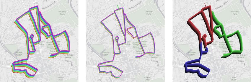
13C.2 Additional Evaluation Examples
Radar Input Predicted Mask Masked Features Correlation Covariance
Figure 8: Additional qualitative examples generated from our best performing model. The masks
generated from our network filter out noise and distractor objects in the scene whilst preserving
temporally consistent features such as walls, well suited for pose prediction. From left to right the
raw Cartesian radar scan, the predicted network mask, the masked radar scan, the correlation volume
and the fitted gaussian to the correlation volume after temperature weighted softmax.
14You can also read