Human Pose Estimation with Spatial Contextual Information
←
→
Page content transcription
If your browser does not render page correctly, please read the page content below
Human Pose Estimation with Spatial Contextual Information

                                                               Hong Zhang1     Hao Ouyang2     Shu Liu3                                Xiaojuan Qi5
                                                                   Xiaoyong Shen3     Ruigang Yang1,4                              Jiaya Jia3,5
                                                     1
                                                    Baidu Research, Baidu Inc. 2 Hong Kong University of Science and Technology
                                               3
                                                 YouTu Lab, Tencent 4 University of Kentucky 5 The Chinese University of Hong Kong
arXiv:1901.01760v1 [cs.CV] 7 Jan 2019

                                                             {fykalviny,ououkenneth,liushuhust,qxj0125,goodshenxy}@gmail.com
                                                                          yangruigang@baidu.com                 leojia@cse.cuhk.edu.hk

                                                                  Abstract                                      needs to learn semantically strong appearance features and
                                                                                                                prevent gradient vanishing during training.
                                            We explore the importance of spatial contextual informa-                Spatial contextual correlation among different joints
                                        tion in human pose estimation. Most state-of-the-art pose               plays an important role in human pose estimation [12, 45].
                                        networks are trained in a multi-stage manner and produce                Fig. 1 shows the prediction maps of different stages. Rough
                                        several auxiliary predictions for deep supervision. With this           locations of head and left knee are easy to identify in the
                                        principle, we present two conceptually simple and yet com-              first stage. However, joints like {right knee, left ankle} in
                                        putational efficient modules, namely Cascade Prediction                 Fig. 1 are with large deformation and occlusion, which are
                                        Fusion (CPF) and Pose Graph Neural Network (PGNN),                      hard to determine only based on the local regions. Fortu-
                                        to exploit underlying contextual information. Cascade pre-              nately, location of joints like left knee is associated with left
                                        diction fusion accumulates prediction maps from previous                ankle. So the prediction result of left knee in the first stage
                                        stages to extract informative signals. The resulting maps               could be indicated as a prior to help infer the location of left
                                        also function as a prior to guide prediction at following               ankle in the following stage.
                                        stages. To promote spatial correlation among joints, our                    Moreover, since human pose estimation is related to
                                        PGNN learns a structured representation of human pose as                structure, it is important to design appropriate guideline to
                                        a graph. Direct message passing between different joints is             choose directions of information propagation for the joints
                                        enabled and spatial relation is captured. These two modules             that are unclear or occluded. Probabilistic Graphical Mod-
                                        require very limited computational complexity. Experimen-               els (PGMs) are used to facilitate message passing among
                                        tal results demonstrate that our method consistently outper-            joints. In [46, 12], MRF or CRF is utilized to describe the
                                        forms previous methods on MPII and LSP benchmark.                       distribution of human body. Nevertheless, the status of each
                                                                                                                joint needs to be sequentially updated, which means before
                                                                                                                updating the status of current joints, status of the previous
                                        1. Introduction                                                         joints is to be refreshed. The sequential nature of the up-
                                                                                                                dating scheme makes it easy to accumulate error. The mul-
                                           Human pose estimation refers to the problem of deter-                tilevel compositional models [56, 43] considered the rela-
                                        mining precise pixel location of important keypoints of hu-             tions of joints. These methods all rely on hierarchy struc-
                                        man body. It serves as a fundamental tool to solve other                tures. Pose grammars are based on the prior knowledge of
                                        high level tasks, such as human action recognition [48,                 the human body.
                                        28], tracking [9, 51] and human-computer interaction [41].                  To make good use of the underlying spatial contextual
                                        There are already a variety of solutions where remaining                information, we propose two conceptually simple and com-
                                        challenges include large change in appearance, uncommon                 putational efficient modules to estimate body joints.
                                        body postures and occlusion.
                                           Recent successful human pose estimation methods are                  Our Contribution #1 To utilize the contextual informa-
                                        based on Convolutional Neural Networks (CNNs). State-                   tion, we propose Cascade Prediction Fusion (CPF) to make
                                        of-the-art methods [35, 50, 52] train pose networks in a                use of auxiliary prediction maps. The prediction maps at
                                        multi-stage fashion. These networks produce several auxil-              previous stage could be deemed as a prior to support predic-
                                        iary prediction maps. Then the predictions are refined itera-           tions in following stages. This procedure is different from
                                        tively in different stages until the final result is produced. It       that of [35, 50], where prediction maps were concatenated

                                                                                                            1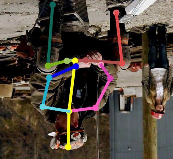
Figure 1. Pipeline of multi-stage prediction. A set of auxiliary predictions are generated. In the first stage, it is easy to identify easy joints
while others with severe deformation are still confusing. Relative positions between joints help resolve ambiguity in the second stage. All
joints converge to the final prediction in the third stage.

with or added to image feature maps and then fed to fol-                    into two groups. The first is to learn feature representa-
lowing huge CNN trunks. As shown in Fig. 2, we create a                     tion using powerful CNN. These methods detect body joint
light-weight path to gradually accumulate auxiliary predic-                 location directly or predict the score maps for body joints.
tion maps for final accurate pose estimation. The predic-                   Early methods like DeepPose [47] regressed joint locations
tions at different stages are with varied properties. Specif-               with multiple stages. Later, Fan et al. [17] combined lo-
ically, predictions from lower layers are with more accu-                   cal and global features to improve performance. To connect
rate localization signals while those at higher layers are with             the input and output space, Carreira et al. [5] iteratively
stronger semantic information to distinguish among similar                  concatenated the input image with previous prediction in
keypoints. Our network effectively fuses information from                   each step. Following the paradigm of semantic segmenta-
different stages by the shorter path created by CPF.                        tion [33, 6], methods of [35, 50, 52] used Gaussian peaks
                                                                            to represent part locations. Then a fully convolutional neu-
Our Contribution #2 We introduce the Pose Graph Neu-
                                                                            ral network [33] is applied to estimate body joint location.
ral Network (PGNN), which is flexible and efficient to learn
                                                                            These methods can produce high quality representation and
a structured representation of body joints. Our PGNN is
                                                                            do not predict structure among body joints, however.
built on a graph that can be integrated in various pose esti-
                                                                               The other group focuses on modeling spatial relationship
mation networks. Each node in the graph is associated with
                                                                            between body joints. The pictorial structures [36] modeled
neighboring body parts. Spatial relations are thus captured
                                                                            spatial deformation by designing pairwise terms between
through edge construction. Direct message passing between
                                                                            different joints. To deal with human poses with large vari-
different nodes is enabled for precise prediction.
                                                                            ation, a mixture model is learned for each joint. Yang et
    Ours is different in modeling spatial relation. PGNN is
                                                                            al. [53] used a part mixture model to infer spatial relation
a novel way to adaptively select the message passing direc-
                                                                            with a tree structure. This structure may not capture very
tions in parallel. Instead of defining an explicit sequential
                                                                            complicated relation. Subsequent methods introduced other
order for a human body structure, it dynamically arranges
                                                                            models, such as loopy structure [49] and poselet [36] to fur-
the update sequences. Via simultaneous update, we manage
                                                                            ther improve the performance.
the short- and long-term relation. Finally, PGNN learns a
                                                                               Later methods [45, 46] modeled structures via CNN.
structured graph representation to boost performance.
                                                                            Tompson et al. [46] utilized the Markov Random
    Our system is also end-to-end trainable, which not only
                                                                            Field (MRF) to model distribution of body parts. Convo-
estimates body location but also configures the spatial struc-
                                                                            lutional priors were used in defining the pairwise terms of
tures. We evaluate the system on two representative hu-
                                                                            joints. The method of [11] utilized geometrical transform
man pose benchmark datasets, i.e., MPII and LSP. It ac-
                                                                            kernels to capture relation of joints on feature maps.
complishes new state-of-the-arts with high computational
efficiency.
                                                                            Graph Neural Network Previous work on feature learn-
                                                                            ing for graph-structure can be divided into two categories.
2. Related Work
                                                                            One direction is to apply CNN to graphs. Based on graph
Human Pose Estimation The key of human pose estima-                         Laplacian, methods of [3, 15, 25] applied CNN to spec-
tion lies in joint detection and spatial relation configuration.            tral domain. In order to operate CNN directly on graph,
Previous human pose estimation methods can be divided                       the method of [16] used a special hash function. The other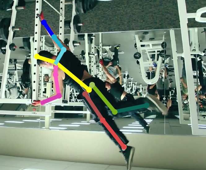
CPF Prediction
                          ...                ...              ...                               ...

                                   pred1
     Input
                                                      pred2                                     pred7
   Elem-wise Sum
                      (a) Cascade Prediction Fusion (CPF)
   Conv + BN + ReLU

                                                                            GRU unit
                                                                                   z

                                                                    Input
                                                                              r
                                                                                       Output

       (c) Tree           (d) Loopy
       Predefined Pose Graph                (b) Pose Graph Neural Network (PGNN)                                           Final Prediction

Figure 2. Framework. Our system takes an image as input, and generates the prediction maps. The architecture is with two components
where CPF is for computing the prediction maps and the other PGNN is for refining these maps until final prediction.

line focuses on recurrently applying neural networks to each                body joints. Our CPF is designed to gradually integrate
node of the graph. State of each node can be updated based                  different semantic information from lower to higher lay-
on history and new information passing through edges. The                   ers. Fig. 2(a) shows the way to incorporate CPF into Hour-
Graph Neural Network (GNN) was first proposed in [40].                      glass [35] framework. It can be built on top of most multi-
It utilized multi-layer perceptrons (MLP) to learn hidden                   stage pose estimation frameworks and iterates from the first
state of nodes in graphs. However, the contraction map                      stage to the final predictions.
assumption is a restriction. As an extension, the Gated
                                                                               For stage i, instead of simply fusing the prediction map
Graph Neural Network (GGNN) [27] adopted recurrent gat-
                                                                            predi−1 from last stage with predi from current stage di-
ing function [8] to update the hidden state and output se-
                                                                            rectly, we provide predi−1 as a prior, which is used for
quences. Parameters of the final model can be effectively
optimized by the back-propagation through time (BPTT) al-                   producing predi . Particularly, the coarse prediction map
                                                                            predi−1 undergoes a 1 × 1 convolution to increase channels
gorithm. Very recently, GGNNs was used in image classifi-
                                                                            and is then merged with image features from stage i by us-
cation [34], situation recognition [26] and RGBD semantic
segmentation [38].                                                          ing element-wise addition. predi is generated by taking the
                                                                            fused feature map as input.
3. Our Method                                                                  CPF is different from DenseNet [22] and DLA [54].
   In this section, we describe the two major components                    DenseNet emphasizes more on feature reuse and gradient
in our method. One is a cascaded multi-stage prediction                     vanish issues. DLA unifies semantic and spatial fusion in
module where previous-stage prediction serves as a prior to                 the feature level. In contrast, CPF focuses on exploring and
guide present prediction and accumulate auxiliary predic-                   aggregating the contextual information encoded in predic-
tion as shown in Fig. 2(a). The other is to model different                 tion maps.
parts in a graph, augmented by Pose Graph Neural Network
(PGNN) to learn representation, as shown in Fig. 2(b).
                                                                            3.2. Graph Neural Network (GNN)
3.1. Cascade Prediction Fusion (CPF)
   For common pose estimation methods [35, 50], a set of                       Graph neural network (GNN) is a general model han-
prediction maps are iteratively refined for body parts. We                  dling graph structured data. GNN takes the graph G =
propose CPF to take the underlying contextual information                   {K, E} as input where K and E represent the nodes and
encoded in auxiliary prediction into consideration.                         edges of the graph respectively. Each node k ∈ K is as-
   These prediction maps are in different semantic levels                   sociated with a hidden state vector hk , which is recurrently
while all of them can be utilized for final predictions. As                 updated. The hidden state vector at time step t is denoted
detailed in [55, 13], the lower-layer features focus on lo-                 as htk . The hidden state is updated by taking as input its
cal appearance and describe details. It is crucial for accu-                current state vector and the incoming messages xtk from its
rate joints localization. Meanwhile, the global representa-                 neighboring nodes Nk . A is a function to collect messages
tions from higher layers help discriminate among different                  from neighboring nodes. T is a function to update the hid-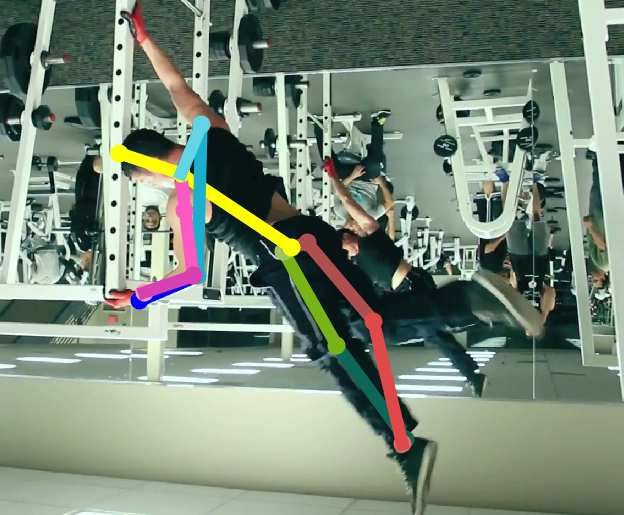
den state. Formally, the hidden state is updated as               Output and Learning After T -time propagation, we get
                                                                  the final prediction
                   xtk = A(ht−1
                            u |u ∈ Nk ),
                                                           (1)
                   htk = T (ht−1  t
                             k , xk ).
                                                                                          Pek = hTk + h0k ,                  (5)

In the following, we present our new GNN named PGNN               where hTk is the final hidden state collected from the corre-
for pose estimation.                                              sponding node. h0k is the initialization hidden state, which
                                                                  encodes the appearance information of a joint. We get the
Graph Construction Each node k in PGNN represents                 final prediction by adding these two prediction maps. The
one body joint and each edge is defined as the connection         graph network is trained by minimizing the ℓ2 loss of
between neighboring joints. Fig. 2(c) shows an example of
                                                                                   K
how to construct a tree-like graph for human poses. The                          1 XX e
                                                                          L2 =           ||Pk (x, y) − Pk (x, y)||2 ,        (6)
prediction maps are treated as unary maps learned from a                         K   x,y
                                                                                    k=1
backbone network, which will be detailed in Sec. 4. The
hidden state of each node is initialized with its correspond-     where (x, y) is the pixel location, Pk (x, y) is the ground
ing spatial prediction feature map derived from the original      truth label at pixel (x, y). Pek is the prediction map obtained
image. The status of node k is initialized as                     in Eq. (5). The model is trained with back-propagation
               h0k = Fk (Θ, I), k ∈ {1 · · · K},           (2)    through time (BPTT).

where F indicates the backbone network, Θ is a set of pa-         3.2.1 Graph Types
rameters for the network, and I is the original input image.
                                                                  PGNN can handle a variety of graphs. It develops a novel
Information Propagation We use the constructed graph              message passing scheme so that each body receives mes-
to exploit the semantic spatial relation and refine the appear-   sage from specific neighboring joints. Intuitively, a fully
ance representation for each joint in steps. Before updating      connected graph is expected to be the ideal choice to collect
the hidden state of each node, it first aggregates messages       information from all other joints. However, for some joints,
of the hidden state at time step t − 1 from neighboring node      such as head and ankle, it is hard to capture the relationship.
k ′ . As demonstrated in [11], convolutional layers can be           To address this problem, we utilize two types of struc-
used as geometrical transform kernels. It advances message        ture, i.e., tree and loopy structure. It is not known before-
passing between feature maps. It is noted that the weights        hand which one is better. A tree is a simple structure, which
of convolution for different edges are not shared. So A is        captures the relation of neighboring joints. Loopy structure
expressed as                                                      is more complex, allowing message passing in a loop. The
                        X                                         structure we use in this paper is illustrated in Fig. 2(c) and
                xtk =        Wp,k ht−1
                                    k′ + bp,k ,             (3)   (d). Although many tree-like or loopy graphs can be de-
                      k,k′ ∈Ω                                     rived, PGNN tackles them in the same way. The graphs are
                                                                  undirected and enable bidirectional message passing.
where Wp,k is the convolution weights and bp,k is the bias
of the k th node. Ω is a set of connected edges.
   Eq. (4) gives the formulation of T . It updates the k th       3.2.2 Relationship to Other Methods
node with the aggregated messages and the t − 1 step of           Most current state-of-the-art methods focus more on ap-
hidden state. We follow the same gating mechanism with            pearance learning of body parts. They capture spatial re-
GRU [27] and enjoy more computational efficiency and less         lation by enlarging the receptive fields. However, poses
memory consumption. Again, we utilize convolution oper-           are with large variation, making the structure information
ations and do not share weights. Wz,k , Uz,k , bz,k , Wr,k ,      in prediction feature maps still have the potential to boost
Ur,k , br,k , Wh,k , Uh,k and bh,k are the weights and biases     the performance. Other models like Recurrent Neural Net-
for the k th node in the update function. With this method,       work (RNN) and Probabilistic Graphical Model (PGM) can
the aggregated information is softly combined with its own        also model the relation. We will detail the difference be-
memory, which can be expressed as                                 tween PGNN and these models in the following.
    zkt = σ(Wz,k xtk + Uz,k ht−1
                             k   + bz,k ),
    rkt = σ(Wr,k xtk + Ur,k ht−1 + br,k ),                        PGNN vs. RNN RNN can be deemed as a special case of
                             k
                                                           (4)    PGNN. It is also able to pass information across nodes of a
    h̃tk = tanh(Wh,k xtk + Uh,k (rkt ⊙ ht−1
                                        k ) + bh,k ),             graph, where each body part is denoted as a node and the
    htk = (1 − zkt ) ⊙ ht−1
                        k   + zkt ⊙ h̃tk .                        joints relations are propagated through edges. However, the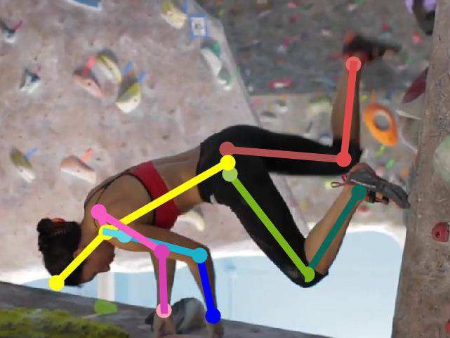
graph structure requires to be chains for RNN. For its con-       and further improve the results using PGNN. The following
struction, at each time step, the state of current node in RNN    two techniques are also used to adapt ResNet-50.
is updated by its current state and the hidden state of the
parent node. It is different from our PGNN, which collects        Feature Pyramid Network (FPN) As introduced in
information from a set of neighboring nodes. Moreover, the        Sec. 3.1, multi-stage prediction is very important for train-
order of RNN input is manually defined. A slightly inap-          ing a pose network. To this end, we adopt Feature Pyra-
propriate setting may destroy the naturally structured rela-      mid Network (FPN) [30] in the vanilla ResNet-50. FPN
tionship of joints.                                               leverages the pyramid shape in networks for prediction at
    Tree-structured RNN [42] can handle tree-structured           different feature levels. Similar to FPN, we also use a lat-
data, which propagates information through a tree sequen-         eral connection (1 × 1 conv) to merge the information from
tially. In addition, before updating the state of subsequent      both bottom-up and top-down pathways. Finally, we pro-
layers Lt , it must update the ancestors Lt−1 at first. Con-      duce three auxiliary predictions at three different levels.
trarily, PGNN updates all states of the node simultaneously.
In addition, RNN shares weights at different time steps. The
                                                                  Dilated Convolution Dilated Convolution [6] is used to
transfer matrix between nodes in the graph is shared through
                                                                  enlarge the receptive field without introducing extra param-
T -time update. Note that in our model, each edge of the
                                                                  eters. An input image is down-sampled 32 times after fed
graph has different transformation weights.
                                                                  into the vanilla ResNet-50. However, the feature map is too
                                                                  coarse to precisely localize the joints. To address this prob-
PGNN vs. PGM PGNN is also closely related to proba-               lem, we first decrease the stride of convolution layers of the
bilistic graphical model, which is widely used for pose es-       last two blocks from 2px to 1px. This results in shrink-
timation [46, 11] to integrate joint associations. In fact, our   ing the receptive field. Since for human pose estimation as
model can be viewed as generalization of these models by          demonstrated in [35, 50], the spatial information needs to
designing specific update. As detailed in [46], for a body        be captured by a large enough area, we replace the 3 × 3
part r, the final marginal likelihood Qe r is defined as
                                                                  convolution layers of the last two blocks with the dilated
                     Y                                            convolution. Finally, we reduce the stride to 8px.
              er = 1
              Q        (qr|v ∗ qv + bv→r ),                (7)
                   Z
                        v∈V
                                                                  Other Implementation Details All models are imple-
where V is a set of neighboring nodes of r. qv is the joint       mented by Torch [14]. We use ImageNet pre-trained model
probability, qr|v is the conditional prior and bv→r is the        as the base and adopt RMSProp [44] to optimize parame-
bias, respectively. Z is the partition function. When the         ters. The network is trained in a total of 250 epochs with
aggregation function is formulated as the product and up-         batch size 8. The initial learning rate is 0.001. It decreased
date function is represented by Eq. (7), PGNN is degraded         by 10 times at the 200th epoch.
to the MRF model. With these derivations, it becomes clear
that PGNN is a more general model to integrate joint asso-        3.3.2 Hourglass
ciations by designing specific graph structure and making
its own way to update and aggregate functions.                    The 8-stack Hourglass (Hg) is adopted as the other back-
                                                                  bone network to verify our method. It is much deeper than
3.3. Backbone Networks                                            ResNet-50 and is widely adopted by many pose estimation
   To verify the generality of our method, we use two back-       frameworks. With CPF and PGNN integrated in Hourglass,
bone networks. One is our modified ResNet-50 [20] and the         we achieve new state-of-the-art results.
other is the widely used 8-stack Hourglass [35].
                                                                  Implementation Details The network is implemented us-
3.3.1 ResNet-50                                                   ing Torch and optimized with RMSProp. The parame-
                                                                  ters are randomly initialized. We train the network in 300
ResNet has demonstrated its power on many high-level              epochs with batch size 6. The learning rate starts at 0.00025
tasks, including object detection [20] and instance segmen-       and decreases by 10 times at the 240th epoch.
tation [19, 31, 32]. To show the generalization ability, we
first modify the ResNet-50 network with a few novel steps         4. Experiments
for human pose estimation. It achieves decent results, even
comparable with using other much deeper networks.                 Datasets We evaluate our CPF and PGNN on two
    Our strategy is to first convert the vanilla ResNet-50 into   representative benchmark datasets, i.e., MPII human
a fully convolutional network by removing the final classifi-     pose dataset (MPII) [1] and extended Leeds Sports
cation and average pooling. We integrate CPF in ResNet-50         Poses (LSP) [24]. MPII contains about 25,000 images with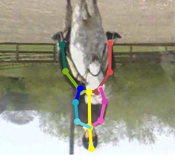
88.6
Mean                                                                87.8                                                                       88.45
                                                                 87.4
                                                                                                 T=3                                            88.43

                               81.1
Ank.               79.3                                                                                                                                  88.61
                 79.0                                                                            T=2
                                                                                                                                                       88.56

                                                    84.6
Knee                                              84.3
                                           83.1                                                                                              88.38
                                                                                                 T=1
                                                                                                                                      88.29
                                                  84.2
Wri.                                      83.1
                                      82.6
                                                                                                                   87 . 82
                                                                                                 T=0               87 . 82
                                                                                  89.5
Elb.                                                                      88.7
                                                                      88.1                           87.4   87.6       87.8    88     88.2       88.4          88.6   88.8
                                                                                                                              Loopy      Tree
   76       78            80          82           84       86             88            90

                    +PGNN-Tree                +CPF         ResNet                             Figure 4. Results at different timesteps with tree-like and loopy-
                                                                                              like structure of PCKh @0.5. The backbone is ResNet-50.
Figure 3. Prediction results of PCKh @0.5 on MPII validation set.
We compare the results by adding CPF and further integrating
PGNN. The backbone is ResNet-50 and PGNN passes message                                       4.1. Ablation Study
with a tree-like structure.
                                                                                                 To investigate the effectiveness of our proposed CPF and
                                                                                              PGNN modules, we conduct ablative analysis on the valida-
over 40,000 annotated poses. We use the same setting as                                       tion set of MPII Human Pose dataset. We set the modified
that in [45] to split training and validation sets. The dataset                               ResNet-50 as our baseline network. To show the efficacy of
is very challenging since it covers daily human activities                                    our models, all results are tested without flipping or multi-
with large pose variety. The LSP dataset consists of 11,000                                   scale testing.
training images and 1,000 testing ones from sport activities.
                                                                                              CPF To evaluate the effectiveness of CPF, we compare
Data Augmentation During training, the input image is                                         results with and without CPF on modified ResNet-50. Fig. 3
cropped and warped to size 256 × 256 according to the an-                                     shows results on MPII validation set. “ResNet” refers to
notated body position and scale. We augment the dataset by                                    our modified ResNet-50. For ResNet-50 with CPF, some
scaling it with a factor ([0.75, 1.25]), rotation (±30), hori-                                difficult joints like knee is 1.2% higher and result of elbow
zontal flipping and illumination adjustment to enhance data                                   is improved by 0.6%.
diversity, and further improve the robustness of the model                                        In order to clearly demonstrate accuracy change in each
for various cases. During testing, we crop the image with                                     stage. Fig. 5(b) shows the accuracy produced at different
the given rough center location and scale of the person. For                                  stages. It is observed that the accuracy increases gradually
LSP dataset, we simply use the size and center of the image                                   in steps on the ResNet. This manifests that our CPF effec-
as rough scale and center.                                                                    tively gathers information from previous predictions.
                                                                                              PGNN Other than adding CPF, we integrate PGNN to fur-
Unary Maps For the two backbone networks, i.e.,                                               ther enhance the accuracy. Fig. 3 gives the experimental
ResNet-50 and Hourglass, we take the last prediction score                                    results where “PGNN” stands for the graph updated twice
maps as the unary maps. The reason is that the prediction at                                  based on a tree-like structure. The accuracy of parts such
the final stage is made based on feature with strong seman-                                   as difficult joints of elbow, wrist is further improved. The
tics, which gathers previous prediction through CPF. It is                                    reason is that the contextual information propagated from
generally with decent prediction accuracy. The score maps                                     confident parts through graph helps reduce error.
are of size H × W × C where H is the height, W is the                                            We use two types of graphs in our experiments. They
width, and C is the channel size. In our experiments, the                                     are tree- and loopy-like graphs in PGNN. Fig. 4 presents the
size of C depends on different datasets. W and H are all                                      results using different PGNN structures. They are compa-
with size 64, which is 1/8 of the original input image.                                       rable – connecting the parts including {elbow, ankle} with
                                                                                              other easy parts consistently improves performance. In our
Evaluation Criteria We use the Percentage Correct Key-                                        experiments, a naive loopy structure, shown in Fig. 2(d),
points (PCK) to evaluate results on the LSP dataset. For                                      is used. We simply add extra connections, i.e. shoulder–
MPII, we use PCKh [1], a modified version of PCK. It nor-                                     wrist, ankle–hip, and shoulder–hip. It is notable that perfor-
malizes the distance errors with respect to the size of head.                                 mance of these two types of graphs with the same number of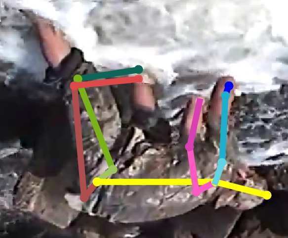
steps are consistent. We thus believe allowing information Methods Head Sho. Elb. Wri. Hip Knee Ank. Mean
Belagiannis&Zisserman [2] 95.2 89.0 81.5 77.0 83.7 87.0 82.8 85.2
to propagate between neighboring joints is of great impor-
Lifshitz et al. [29] 96.8 89.0 82.7 79.1 90.9 86.0 82.5 86.7
tance. More sophisticated structures may further improve Pishchulin et al. [37] 97.0 91.0 83.8 78.1 91.0 86.7 82.0 87.1
the performance, which will be our future work. Insafutdinov et al. [23] 97.4 92.7 87.5 84.4 91.5 89.9 87.2 90.1
Wei et al. [50] 97.8 92.5 87.0 83.9 91.5 90.8 89.9 90.5
We also conduct experiments to compare results when Bulat&Tzimiropoulos [4] 97.2 92.1 88.1 85.2 92.2 91.4 88.7 90.7
propagating different times (i.e. with varying propagation Yang et al. [52] 98.3 94.5 92.2 88.9 94.4 95.0 93.7 93.9
number T ) in the system. The results are shown in Fig. 4. ResNet-ours 98.5 94.0 89.9 86.9 92.3 93.5 92.7 92.5
The performance increases by a small amount when in- Hg-ours 98.4 94.8 92.0 89.4 94.4 94.8 93.8 94.0
creasing T , and saturates quickly at T = 3. We also notice
Table 2. Comparison of PCK @0.2 on the LSP dataset. ResNet
that propagation is important in the first 2 steps. For the is short for ResNet-50. Both backbones are trained with CPF and
tree-like graph, as revealed in the comparison when apply- PGNN.
ing T = 0, T = 1 and T = 2, we obtain the improvement
of around 0.5% and 0.3%, respectively. Similar results are
observed when using the loopy-like graph. However, the
performance begins to drop at T = 3. Since it is hard Complexity In Fig. 5(a), we compare the number of pa-
to capture the semantic information between too far away rameters and computational complexity between Hourglass,
joints, but instead confuses prediction at current joint. previous method PRM [52] and our model. We note that the
PRM adds 13.5% extra parameters compared with Hour-
glass, while our model only increases parameters by 0.8%.
Methods Head Sho. Elb. Wri. Hip Knee Ank. Mean
Pishchulin et al. [36] 74.3 49.0 40.8 34.1 36.5 34.4 35.2 44.1
Additionally, we introduce very limited computation over-
Tompson et al. [46] 95.8 90.3 80.5 74.3 77.6 69.7 62.8 79.6 head (measured by GFLOPs) on Hourglass, contrary to
Carreira et al. [5] 95.7 91.7 81.7 72.4 82.8 73.2 66.4 81.3 much increased computational cost from PRM. Our results
Tompson et al. [45] 96.1 91.9 83.9 77.8 80.9 72.3 64.8 82.0 are with higher quality and decent computational efficiency.
Hu&Ramanan et al. [21] 95.0 91.6 83.0 76.6 81.9 74.5 69.5 82.4
Pishchulin et al. [37] 94.1 90.2 83.4 77.3 82.6 75.7 68.6 82.4
Lifshitz et al. [29] 97.8 93.3 85.7 80.4 85.3 76.6 70.2 85.0
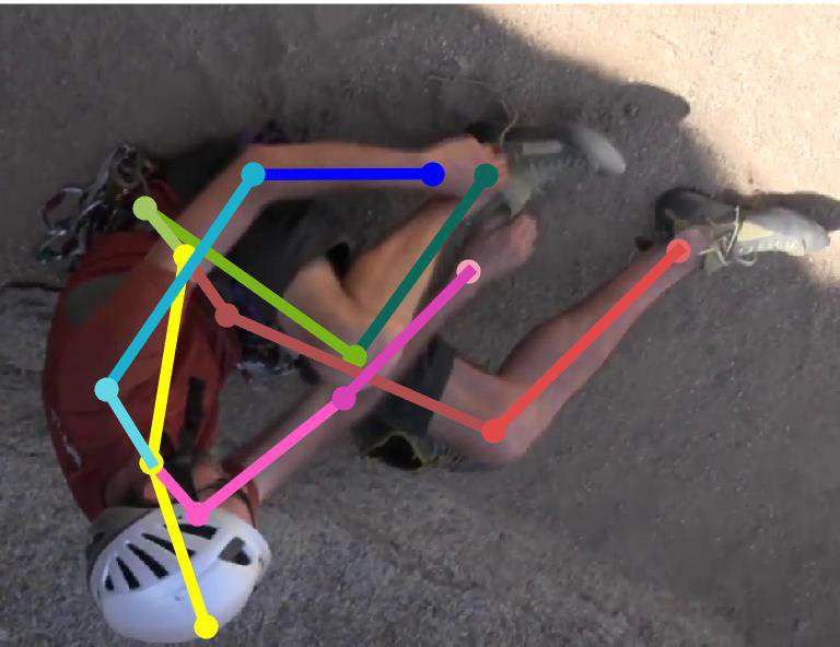
Visual Analysis In Fig. 6, we visualize results of baseline
Gkioxary et al. [18] 96.2 93.1 86.7 82.1 85.2 81.4 74.1 86.1 and our model. The baseline model has difficulty in distin-
Rafi et al. [39] 97.2 93.9 86.4 81.3 86.8 80.6 73.4 86.3 guishing among symmetric parts and uncommon body pos-
Insafutdinov et al. [23] 96.8 95.2 89.3 84.4 88.4 83.4 78.0 88.5 tures. For example, in {col.1, row.2} of Fig. 6, ankle with
Wei et al. [50] 97.8 95.0 88.7 84.0 88.4 82.8 79.4 88.5
Chu et al. [13] 98.5 96.3 91.9 88.1 90.6 88.0 85.0 91.5
large deformation is hard to identify with inherent ambigu-
Chou et al. [10] 98.2 96.8 92.2 88.0 91.3 89.1 84.9 91.8 ity. Our proposed CPF and PGNN provide an effective way
Chen et al. [7] 98.1 96.5 92.5 88.5 90.2 89.6 86.0 91.9 to utilize contextual information to reduce the confusion.
Yang et al. [52] 98.5 96.7 92.5 88.7 91.1 88.6 86.0 92.0 As a result, the associated joints knee help inferring the pre-
Newell et al. [35] 98.2 96.3 91.2 87.1 90.1 87.4 83.6 90.9 cise location of ankle in our model as shown in {col.2 and
ResNet-ours 98.2 96.4 91.6 87.1 91.2 88.0 83.6 91.2
Hg-ours 98.6 97.0 92.8 88.8 91.7 89.8 86.6 92.5 row.2} of Fig 6. More results on MPII and LSP generated
by our method are shown in Fig. 7.
Table 1. Results of PCKh @0.5 on the MPII test set. Note that
ResNet is our modified ResNet-50. ResNet-50 and Hg are all 4.3. Experimental Results on LSP
trained with CPF and PGNN.
Tab. 2 gives comparison with person-centric annotation.
The results are evaluated with PCK scores at threshold 0.2.
Following previous methods [13, 52], we add the MPII
4.2. Experimental Results on MPII training set to the extended LSP training set. Our modified
ResNet-50 outperforms most of the methods trained with
Accuracy Tab. 1 lists our results on MPII test set. “Hg- deeper networks.
ours” is trained on MPII combined with LSP. The results
are produced with five-scale input with horizontal flip test- 5. Concluding Remarks
ing. Our method trained based on Hourglass yields result
92.5% PCKh at threshold 0.5, which is the highest on this We have presented effective Cascade Prediction Fusion
dataset at the time of paper submission. For the challeng- (CPF) and Pose Graph Neural Network (PGNN) to ex-
ing parts such as knee and ankle, we obtain improvement of plore contextual information for human pose estimation.
2.4% and 3.0% compared to the baseline Hourglass, respec- CPF makes use of rich contextual information encoded in
tively. Particularly, our method outperforms the method the auxiliary score maps to produce enhanced prediction.
[13] with CRF as well. It is noteworthy that accuracy of PGNN, differently, is adopted to provide an explicit infor-
our method (ResNet-ours) is also higher than the baseline mation propagation scheme to refine prediction. These two
ResNet-50, which proves the generalization ability. components are independent while beneficial to each other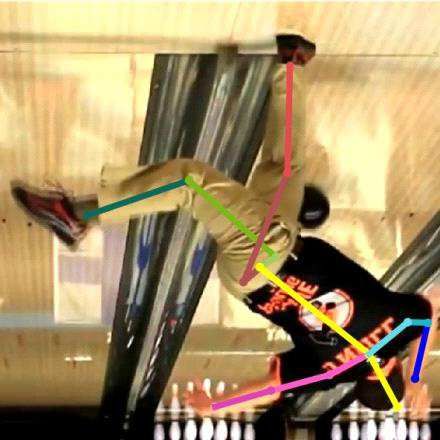
Parameters Complexity Accuracy 88.5
28 47 93.0 ResNet
46 45.9 92.5 88.0 ResNet+CPF 87.8
26.9
#Params (Million)
27 92.5 87.6
45
87.5 87.4 87.4
PCKh@0.5
92.0
Accuracy
26 44 92.0
GFLOPs
43 87.0
25 91.5 86.7
42 86.6
41.2 41.4 86.5
23.9 41 91.0 90.9
24 23.7
40 86.0
23 90.5
39
90.0 85.5
22 38 1 2 3
Hg PRM Ours Hg PRM Ours Hg PRM Ours Stage
(a) (b)
Figure 5. (a) Statistics of parameter numbers, GFLOPs and accuracy on three frameworks, i.e., baseline Hourglass, PRM and our method
respectively. (b) Prediction accuracy at different stages with modified ResNet-50.
2016. 2, 7
[6] L.-C. Chen, G. Papandreou, I. Kokkinos, K. Murphy, and
A. L. Yuille. Deeplab: Semantic image segmentation with
deep convolutional nets, atrous convolution, and fully con-
nected crfs. arXiv preprint arXiv:1606.00915, 2016. 2, 5
[7] Y. Chen, C. Shen, X.-S. Wei, L. Liu, and J. Yang. Adversarial
posenet: A structure-aware convolutional network for human
pose estimation. arXiv preprint arXiv:1705.00389, 2017. 7
[8] K. Cho, B. Van Merriënboer, C. Gulcehre, D. Bahdanau,
F. Bougares, H. Schwenk, and Y. Bengio. Learning phrase
representations using rnn encoder-decoder for statistical ma-
chine translation. arXiv preprint arXiv:1406.1078, 2014. 3
[9] N.-G. Cho, A. L. Yuille, and S.-W. Lee. Adaptive occlu-
sion state estimation for human pose tracking under self-
occlusions. Pattern Recognition, 46(3):649–661, 2013. 1
[10] C.-J. Chou, J.-T. Chien, and H.-T. Chen. Self adversar-
Hg Hg-ours ResNet ResNet-ours ial training for human pose estimation. arXiv preprint
arXiv:1707.02439, 2017. 7
Figure 6. Results on MPII test set produced by different backbone [11] X. Chu, W. Ouyang, H. Li, and X. Wang. Structured feature
networks, i.e. Hourglass and ResNet-50. Hg-ours and ResNet-50- learning for pose estimation. In CVPR, 2016. 2, 4, 5
ours are both trained with CPF and PGNN. [12] X. Chu, W. Ouyang, X. Wang, et al. Crf-cnn: Modeling
structured information in human pose estimation. In NIPS,
2016. 1
in human pose estimation. They are also general for most [13] X. Chu, W. Yang, W. Ouyang, C. Ma, A. L. Yuille, and
existing pose estimation networks to boost performance. X. Wang. Multi-context attention for human pose estima-
Our future work will be to extend our framework to 3D tion. arXiv preprint arXiv:1702.07432, 2017. 3, 7
and video data for deeper understanding of the temporal and [14] R. Collobert, K. Kavukcuoglu, and C. Farabet. Torch7: A
spatial relationship. matlab-like environment for machine learning. In BigLearn,
NIPS Workshop, 2011. 5
References [15] M. Defferrard, X. Bresson, and P. Vandergheynst. Convolu-
tional neural networks on graphs with fast localized spectral
[1] M. Andriluka, L. Pishchulin, P. Gehler, and B. Schiele. 2d filtering. In NIPS, 2016. 2
human pose estimation: New benchmark and state of the art [16] D. K. Duvenaud, D. Maclaurin, J. Iparraguirre, R. Bom-
analysis. In CVPR, 2014. 5, 6 barell, T. Hirzel, A. Aspuru-Guzik, and R. P. Adams. Con-
[2] V. Belagiannis and A. Zisserman. Recurrent human pose volutional networks on graphs for learning molecular finger-
estimation. In FG, 2017. 7 prints. In NIPS, 2015. 2
[3] J. Bruna, W. Zaremba, A. Szlam, and Y. LeCun. Spectral [17] X. Fan, K. Zheng, Y. Lin, and S. Wang. Combining local
networks and locally connected networks on graphs. arXiv appearance and holistic view: Dual-source deep neural net-
preprint arXiv:1312.6203, 2013. 2 works for human pose estimation. In CVPR, 2015. 2
[4] A. Bulat and G. Tzimiropoulos. Human pose estimation via [18] G. Gkioxari, A. Toshev, and N. Jaitly. Chained predictions
convolutional part heatmap regression. In ECCV, 2016. 7 using convolutional neural networks. In ECCV, 2016. 7
[5] J. Carreira, P. Agrawal, K. Fragkiadaki, and J. Malik. Hu- [19] K. He, G. Gkioxari, P. Dollár, and R. Girshick. Mask r-cnn.
man pose estimation with iterative error feedback. In CVPR, In ICCV, 2017. 5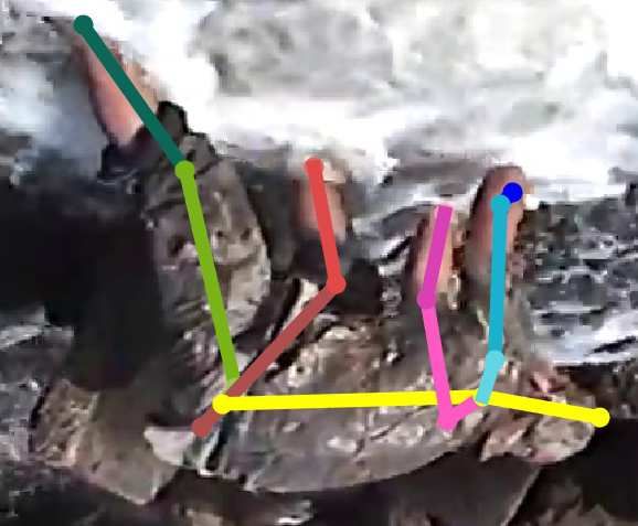
Figure 7. Example output on the LSP and MPII test data.

[20] K. He, X. Zhang, S. Ren, and J. Sun. Deep residual learning       [34] K. Marino, R. Salakhutdinov, and A. Gupta. The more you
     for image recognition. In CVPR, 2016. 5                                know: Using knowledge graphs for image classification. In
[21] P. Hu and D. Ramanan. Bottom-up and top-down reasoning                 CVPR, 2017. 3
     with hierarchical rectified gaussians. In CVPR, 2016. 7           [35] A. Newell, K. Yang, and J. Deng. Stacked hourglass net-
[22] G. Huang, Z. Liu, K. Q. Weinberger, and L. van der Maaten.             works for human pose estimation. In ECCV, 2016. 1, 2, 3,
     Densely connected convolutional networks. In CVPR, 2017.               5, 7
     3                                                                 [36] L. Pishchulin, M. Andriluka, P. Gehler, and B. Schiele. Pose-
                                                                            let conditioned pictorial structures. In CVPR, 2013. 2, 7
[23] E. Insafutdinov, L. Pishchulin, B. Andres, M. Andriluka, and
                                                                       [37] L. Pishchulin, E. Insafutdinov, S. Tang, B. Andres, M. An-
     B. Schiele. Deepercut: A deeper, stronger, and faster multi-
                                                                            driluka, P. Gehler, and B. Schiele. Deepcut: Joint subset
     person pose estimation model. In ECCV, 2016. 7
                                                                            partition and labeling for multi person pose estimation. In
[24] S. Johnson and M. Everingham. Clustered pose and nonlin-               CVPR, 2016. 7
     ear appearance models for human pose estimation. In BMVC,
                                                                       [38] X. Qi, R. Liao, J. Jia, S. Fidler, and R. Urtasun. 3d graph
     2010. 5
                                                                            neural networks for rgbd semantic segmentation. In ICCV,
[25] T. N. Kipf and M. Welling. Semi-supervised classifica-                 2017. 3
     tion with graph convolutional networks. arXiv preprint            [39] U. Rafi, B. Leibe, J. Gall, and I. Kostrikov. An efficient
     arXiv:1609.02907, 2016. 2                                              convolutional network for human pose estimation. In BMVC,
[26] R. Li, M. Tapaswi, R. Liao, J. Jia, R. Urtasun, and S. Fidler.         2016. 7
     Situation recognition with graph neural networks. In ICCV,        [40] F. Scarselli, M. Gori, A. C. Tsoi, M. Hagenbuchner, and
     2017. 3                                                                G. Monfardini. The graph neural network model. IEEE
[27] Y. Li, D. Tarlow, M. Brockschmidt, and R. Zemel. Gated                 Transactions on Neural Networks, 20(1):61–80, 2009. 3
     graph sequence neural networks. In ICLR, 2016. 3, 4               [41] J. Shotton, T. Sharp, A. Kipman, A. Fitzgibbon, M. Finoc-
[28] Z. Liang, X. Wang, R. Huang, and L. Lin. An expressive                 chio, A. Blake, M. Cook, and R. Moore. Real-time human
     deep model for human action parsing from a single image.               pose recognition in parts from single depth images. Commu-
     In ICME, 2014. 1                                                       nications of the ACM, 56(1):116–124, 2013. 1
[29] I. Lifshitz, E. Fetaya, and S. Ullman. Human pose estimation      [42] K. S. Tai, R. Socher, and C. D. Manning. Improved semantic
     using deep consensus voting. In ECCV, 2016. 7                          representations from tree-structured long short-term memory
                                                                            networks. arXiv preprint arXiv:1503.00075, 2015. 5
[30] T.-Y. Lin, P. Dollár, R. Girshick, K. He, B. Hariharan, and
                                                                       [43] Y. Tian, C. L. Zitnick, and S. G. Narasimhan. Exploring the
     S. Belongie. Feature pyramid networks for object detection.
                                                                            spatial hierarchy of mixture models for human pose estima-
     In CVPR, 2017. 5
                                                                            tion. In ECCV, 2012. 1
[31] S. Liu, J. Jia, S. Fidler, and R. Urtasun. Sgn: Sequen-           [44] T. Tieleman and G. Hinton. Lecture 6.5-rmsprop: Di-
     tial grouping networks for instance segmentation. In ICCV,             vide the gradient by a running average of its recent magni-
     2017. 5                                                                tude. COURSERA: Neural networks for machine learning,
[32] S. Liu, L. Qi, H. Qin, J. Shi, and J. Jia. Path aggregation            4(2):26–31, 2012. 5
     network for instance segmentation. In CVPR, 2018. 5               [45] J. Tompson, R. Goroshin, A. Jain, Y. LeCun, and C. Bregler.
[33] J. Long, E. Shelhamer, and T. Darrell. Fully convolutional             Efficient object localization using convolutional networks. In
     networks for semantic segmentation. In CVPR, 2015. 2                   CVPR, 2015. 1, 2, 5, 7
[46] J. J. Tompson, A. Jain, Y. LeCun, and C. Bregler. Joint train-
     ing of a convolutional network and a graphical model for
     human pose estimation. In NIPS, 2014. 1, 2, 5, 7
[47] A. Toshev and C. Szegedy. Deeppose: Human pose estima-
     tion via deep neural networks. In CVPR, 2014. 2
[48] C. Wang, Y. Wang, and A. L. Yuille. An approach to pose-
     based action recognition. In CVPR, 2013. 1
[49] Y. Wang, D. Tran, and Z. Liao. Learning hierarchical pose-
     lets for human parsing. In CVPR, 2011. 2
[50] S.-E. Wei, V. Ramakrishna, T. Kanade, and Y. Sheikh. Con-
     volutional pose machines. In CVPR, 2016. 1, 2, 3, 5, 7
[51] B. Xiaohan Nie, C. Xiong, and S.-C. Zhu. Joint action recog-
     nition and pose estimation from video. In CVPR, 2015. 1
[52] W. Yang, S. Li, W. Ouyang, H. Li, and X. Wang. Learning
     feature pyramids for human pose estimation. In ICCV, 2017.
     1, 2, 7
[53] Y. Yang and D. Ramanan. Articulated pose estimation with
     flexible mixtures-of-parts. In CVPR, 2011. 2
[54] F. Yu, D. Wang, and T. Darrell. Deep layer aggregation.
     arXiv preprint arXiv:1707.06484, 2017. 3
[55] M. D. Zeiler and R. Fergus. Visualizing and understanding
     convolutional networks. In ECCV, 2014. 3
[56] L. L. Zhu, Y. Chen, and A. Yuille. Recursive compositional
     models for vision: Description and review of recent work.
     Journal of Mathematical Imaging and Vision, 41(1-2):122,
     2011. 1
You can also read