TrafficPredict: Trajectory Prediction for Heterogeneous Traffic-Agents
←
→
Page content transcription
If your browser does not render page correctly, please read the page content below
TrafficPredict: Trajectory Prediction for Heterogeneous Traffic-Agents

                                            Yuexin Ma1,2 , Xinge Zhu3 , Sibo Zhang1 , Ruigang Yang1 , Wenping Wang2 , Dinesh Manocha4
                                                                          Baidu Research, Baidu Inc.1 , The University of Hong Kong2 ,
                                                                 The Chinese University of Hong Kong3 , University of Maryland at College Park4
                                                                      yxma@cs.hku.hk, zhuxinge123@gmail.com, sibozhang@baidu.com,
                                                                        yangruigang@baidu.com, wenping@cs.hku.hk, dm@cs.umd.edu
arXiv:1811.02146v5 [cs.CV] 9 Apr 2019

                                                                    Abstract
                                          To safely and efficiently navigate in complex urban traffic, au-
                                          tonomous vehicles must make responsible predictions in re-
                                          lation to surrounding traffic-agents (vehicles, bicycles, pedes-
                                          trians, etc.). A challenging and critical task is to explore the
                                          movement patterns of different traffic-agents and predict their
                                          future trajectories accurately to help the autonomous vehicle
                                          make reasonable navigation decision. To solve this problem,
                                          we propose a long short-term memory-based (LSTM-based)
                                          realtime traffic prediction algorithm, TrafficPredict. Our ap-
                                          proach uses an instance layer to learn instances’ movements
                                          and interactions and has a category layer to learn the simi-
                                          larities of instances belonging to the same type to refine the
                                          prediction. In order to evaluate its performance, we collected
                                          trajectory datasets in a large city consisting of varying con-
                                          ditions and traffic densities. The dataset includes many chal-
                                          lenging scenarios where vehicles, bicycles, and pedestrians
                                          move among one another. We evaluate the performance of
                                          TrafficPredict on our new dataset and highlight its higher ac-
                                          curacy for trajectory prediction by comparing with prior pre-
                                          diction methods.

                                                                                                             Figure 1: Heterogeneous urban traffic scenario: We
                                                                Introduction                                 demonstrate the improved trajectory prediction accuracy of
                                        Autonomous driving is a significant and difficult task that          our method over prior approaches (top). The green solid
                                        has the potential to impact peoples day-to-day lives. The            lines denote ground truth trajectories (GT), pink solid lines
                                        goal is to make a vehicle perceive the environment and               are for our method (TP) and dashed lines are the predicted
                                        safely and efficiently navigate any traffic situation without        trajectories for other methods (ED, SL, SA). We observe
                                        human intervention. Some of the challenges arise in dense            20% improvement in accuracy using TP. Traffic correspond-
                                        urban environments, where the traffic consists of differ-            ing point cloud captured by LiDAR of the acquisition car
                                        ent kinds of traffic-agents, including cars, bicycles, buses,        is shown on the left bottom. Original trajectories of traffic-
                                        pedestrians, etc.. These traffic-agents have different shapes,       agents in the scenario are shown on the right bottom: blue
                                        dynamics, and varying behaviors and can be regarded as an            for cars, green for bicycles, and red for pedestrians.
                                        instance of a heterogeneous multi-agent system. To guaran-
                                        tee the safety of autonomous driving, the system should be           time, traffic-agents behaviors are deeply affected by other
                                        able to analyze the motion patterns of other traffic-agents          traffic-agents. It is necessary to consider the interaction be-
                                        and predict their future trajectories so that the autonomous         tween the agent to improve the accuracy of trajectory pre-
                                        vehicle can make appropriate navigation decisions.                   diction.
                                           Driving in an urban environment is much more chal-                   The problem of predicting trajectories for moving agents
                                        lenging than driving on a highway. Urban traffic is riddled          has been studied extensively. Some traditional algorithms
                                        with more uncertainties, complex road conditions, and di-            are based on motion models like kinematic and dy-
                                        verse traffic-agents, especially on some cross-roads. Differ-        namic models (Toledo-Moreo and Zamora-Izquierdo 2009),
                                        ent traffic-agents have different motion patterns. At the same       Bayesian filters (Kalman 1960), Gaussian Processes (Ras-
                                                                                                             mussen and Williams 2006), etc. These methods do not take
                                        Copyright c 2019, Association for the Advancement of Artificial      into account interactions between the traffic-agents and the
                                        Intelligence (www.aaai.org). All rights reserved.                    environment, making it difficult to analyze complicated sce-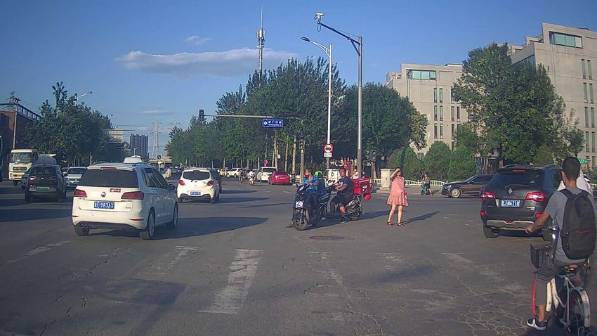
narios or perform long-term predictions. With the success                               Related Work
of LSTM networks in modeling non-linear temporal depen-
dencies (Ma et al. 2017) in sequence learning and genera-          Classical methods for trajectory prediction
tion tasks, more and more works have been using these net-         The problem of trajectory prediction or path prediction
works to predict trajectories of human crowds(Alahi et al.         has been extensively studied. There are many classical
2016) and vehicles trajectories (Lee et al. 2017). The com-        approaches, including Bayesian networks (Lefèvre et al.
mon limitation of these works is the focus on predicting one       2011), Monte Carlo Simulation (Danielsson et al. 2007),
type of group (only pedestrians or cars, for example). These       Hidden Markov Models (HMM) (Firl et al. 2012), Kalman
methods may not work in heterogeneous traffic, where dif-          Filters (Kalman 1960), linear and non-linear Gaussian Pro-
ferent vehicles and pedestrians coexist and interact with each     cess regression models (Rasmussen and Williams 2006), etc.
other(Chandra et al. 2018b).                                       These methods focus on analyzing the inherent regularities
Main Results: For the task of trajectory prediction in het-        of objects themselves based on their previous movements.
erogeneous traffic, we propose a novel LSTM-based algo-            They can be used in simple traffic scenarios in which there
rithm, TrafficPredict. Given a sequence of trajectory data,        are few interactions among cars, but these methods may not
we construct a 4D Graph, where two dimensions are for in-          work well when different kinds of vehicles and pedestrians
stances and their interactions, one dimension is for time se-      appear at the same time.
ries, and one dimension is for high-level categorization. In
this graph, all the valid instances and categories of traffic-     Behavior modeling and interactions
agents are denoted as nodes, and all the relationships in          There is considerable work on human behavior and interac-
spatial and temporal space is represented as edges. Sequen-        tions. The Social Force model (Helbing and Molnar 1995)
tial movement information and interaction information are          presents a pedestrian motion model with attractive and re-
stored and transferred by these nodes and edges. Our LSTM          pulsive forces, which has been extended by (Yamaguchi et
network architecture is constructed on the 4D Graph, which         al. 2011). Some similar methods have also been proposed
can be divided into two main layers: one is the instance layer     that use continuum dynamics (Treuille et al. 2006), Gaus-
and the other is the category layer. The former is designed to     sian processes (Wang et al. 2008), etc. Bera et al. (2016;
capture dynamic properties and and interactions between the        2017) combine an Ensemble Kalman Filter and human mo-
traffic-agents at a micro level. The latter aims to conclude the   tion model to predict the trajectories for crowds. These
behavior similarities of instances of the same category using      methods are useful for analyzing motions of pedestrians in
a macroscopic view and guide the prediction for instances in       different scenarios, such as shopping malls, squares, and
turn. We also use a self attention mechanism in the category       pedestrian streets. There are also some approaches to clas-
layer to capture the historical movement patterns and high-        sify group emotions or identify driver behaviors (Cheung et
light the category difference. Our method is the first to inte-    al. 2018). To extend these methods to general traffic sce-
grate the trajectory prediction for different kinds of traffic-    narios, (Ma et al. 2018) predicts the trajectories of multiple
agents in one unified framework.                                   traffic-agents by considering kinematic and dynamic con-
   To better expedite research progress on prediction and          straints. However, this model assumes perfect sensing and
navigation in challenging scenarios for autonomous driving,        shape and dynamics information for all of the traffic agents.
we provide a new trajectory dataset for complex urban traf-
fic with heterogeneous traffic-agents during rush hours. Sce-      RNN networks for sequence prediction
nario and data sample of our dataset is shown in Fig. 1. In
                                                                   In recent years, the concept of the deep neural network
practice, TrafficPredict takes about a fraction of a second on
                                                                   (DNN) has received a huge amount of attention due to its
a single CPU core and exhibits 20% accuracy improvement
                                                                   good performance in many areas (Goodfellow et al. 2016).
over prior prediction schemes. The novel components of our
                                                                   Recurrent neural network (RNN) is one of the DNN archi-
work include:
                                                                   tectures and is widely used for sequence generation in many
                                                                   domains, including speech recognition (Graves and Jaitly
• Propose a new approach for trajectory prediction in het-         2014), machine translation (Chung et al. 2015), and image
  erogeneous traffic.                                              captioning (Vinyals et al. 2015). Many methods based on
                                                                   long short-term Memory (LSTM), one variant of RNN, have
• Collect a new trajectory dataset in urban traffic with much      been proposed for maneuver classification (Khosroshahi
  interaction between different categories of traffic-agents.      2017) and trajectory prediction (Altché and Fortelle 2017).
                                                                   Some methods (Kim et al. 2017; Park et al. 2018; Lee et al.
• Our method has smaller prediction error compared with            2017) produce the probabilistic information about the future
  other state-of-art approaches.                                   locations of vehicles over an occupancy grid map or sam-
                                                                   ples by making use of an encoder-decoder structure. How-
   The rest of the paper is organized as follows. We give a        ever, these sampling-based methods suffer from inherent in-
brief overview of related prior work in Section 2. In Section      accuracies due to discretization limits. Another method (Deo
3, we define the problem and give details of our prediction        and Trivedi 2018) presents a model that outputs the multi-
algorithm. We introduce our new traffic dataset and show the       modal distribution and then generates trajectories. Never-
performance of our methods in Section 4.                           theless, most of these methods require clear road lanes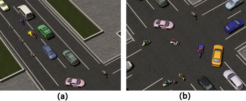
Instance Layer                                  Category Layer

                                           frame n                    frame n+1                 frame n                  frame n+1
                (a)                                       (b)                                                 (c)

Figure 2: Our 4D Graph for a traffic sequence. (a) Icons for instances and categories are shown on the left table. (b) The instance
layer of the 4D Graph with spatial edges as solid lines and temporal edges as dashed lines. (c) The category layer with temporal
edges of super nodes drawn by dashed lines.
and simple driving scenarios without other types of traffic-         Problem Definition
agents passing through. Based on images, (Chandra et al.
                                                                     We assume each scene is preprocessed to get the categories
2018a) models the interactions between different traffic-
                                                                     and spatial coordinates of traffic-agents. At any time t, the
agents by a LSTM-CNN hybrid network for trajectory pre-
                                                                     feature of the ith traffic-agent Ati can be denoted as fit =
diction. Taking into account the human-human interactions,
                                                                     (xti , yit , cti ), where the first two items are coordinates in the
some approaches (Alahi et al. 2016; Gupta et al. 2018;
                                                                     x-axis and y-axis respectively, and the last item is the cate-
Vemula et al. 2017) use LSTM for predicting trajectories
                                                                     gory of the traffic-agent. In our dataset, we currently take
of pedestrians in a crowd and they show good performance
                                                                     into account three types of traffic-agents, ci ∈ {1, 2, 3},
on public crowd datasets. However, these methods are also
                                                                     where 1 stands for pedestrians, 2 represents bicycles and 3
limited in terms of trajectory prediction in complex traffic
                                                                     denotes cars. Our approach can be easily extended to take
scenarios where the interactions are among not only pedes-
                                                                     into account more agent types. Our task is to observe fea-
trians but also heterogeneous traffic-agents.
                                                                     tures of all the traffic-agents in the time interval [1 : Tobs ]
                                                                     and then predict their discrete positions at [Tobs + 1 : Tpred ].
Traffic datasets
                                                                     4D Graph Generation
There are several datasets related to traffic scenes.
Cityscapes (Cordts et al. 2016) contains 2D semantic,                In urban traffic scenarios where various traffic-agents are
instance-wise, dense pixel annotations for 30 classes. Apol-         interacting with others, each instance has its own state in
loScape (Huang et al. 2018) is a large-scale comprehensive           relation to the interaction with others at any time and they
dataset of street views that contains higher scene complexi-         also have continuous information in time series. Consid-
ties, 2D/3D annotations and pose information, lane markings          ering traffic-agents as instance nodes and relationships as
and video frames. However these two dataset do not provide           edges, we can construct a graph in the instance layer, shown
trajectories information. The Simulation (NGSIM) dataset             in Fig.2 (b). The edge between two instance nodes in one
(Administration 2005) has trajectory data for cars, but the          frame is called spatial edge (Jain et al. 2016; Vemula et
scene is limited to highways with similar simple road con-           al. 2017), which can transfer the interaction information
ditions. KITTI (Geiger et al. 2013) is a dataset for different       between two traffic-agents in spatial space. The edge be-
computer vision tasks such as stereo, optical ow, 2D/3D ob-          tween the same instance in adjacent frames is the temporal
ject detection, and tracking. However, the total time of the         edge, which is able to pass the historic information frame
dataset with tracklets is about 22 minutes. In addition, there       by frame in temporal space. The feature of the spatial edge
are few intersection between vehicles, pedestrians and cy-           (Ati , Atj ) for Ati can be computed as fij t
                                                                                                                    = (xtij , yij
                                                                                                                               t
                                                                                                                                  , ctij ),
                                                                                 t       t    t   t       t    t
clists in KITTI, which makes it insufficient for exploring the       where xij = xj − xi , yij = yj − yi stands for the rela-
motion patterns of traffic-agents in challenging traffic con-        tive position from Atj to Ati , ctij is an unique encoding for
ditions. There are some pedestrian trajectory datasets like          (Ati , Atj ). When traffic-agent Aj considers the spatial edge,
ETH (Pellegrini et al. 2009), UCY (Lerner et al. 2007),              the spatial edge is represented as (Atj , Ati ). The feature of
etc., but such datasets only focus on human crowds without
any vehicles.                                                        the temporal edge (Ati , At+1
                                                                                                 i   ) is computed in the same way.
                                                                        It is normally observed that the same kind of traffic-
                                                                     agents have similar behavior characteristics. For example,
                      TrafficPredict                                 the pedestrians have not only similar velocities but also simi-
                                                                     lar reactions to other nearby traffic-agents. These similarities
In this section, we present our novel algorithm to predict the       will be directly reflected in their trajectories. We construct a
trajectories of different traffic-agents.                            super node Cut , u ∈ {1, 2, 3} for each kind of traffic-agent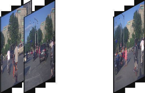
to learn the similarities of their trajectories and then utilize
that super node to refine the prediction for instances. Fig.2          Φ
(c) shows the graph in the category layer. All instances of
the same type are integrated into one group and each group
has an edge oriented toward the corresponding super node.
After summarizing the motion similarities, the super node
                                                                       Φ
passes the guidance through an oriented edge to the group of
instances. There are also temporal edges between the same                                                      Φ

super node in sequential frames. This category layer is spe-
cially designed for heterogeneous traffic and can make full
use of the data to extract valuable information to improve             Φ
the prediction results. This layer is very flexible and can be
easily degenerated to situations when several categories dis-
appear in some frames.
   Finally, we get the 4D Graph for a traffic sequence with
                                                                   Figure 3: Architecture of the network for one super node in
two dimensions for traffic-agents and their interactions, one
                                                                   the category layer.
dimension for time series, and one dimension for high-level
categories. By this 4D Graph, we construct an information
network for the entire traffic. All the information can be         where Wi and Wij are embedding weights, Dot(·) is the dot
delivered and utilized through the nodes and edges of the          product, and √md is a scaling factor (Vaswani et al. 2017).
                                                                                      e
graph.                                                             The final weights are ratios of w(htij ) to the sum. The out-
                                                                   put vector Hit is computed as a weighted sum of htij . Hit
Model Architecture                                                 stands for the influence exhibited on an instance’s trajectory
Our TrafficPredict algorithm is based on the 4D Graph,             by surrounding traffic-agents and htii denotes the informa-
which consists of two main layers: the instance layer and          tion passing by temporal edges. We concatenate them and
the category layer. Details are given below.                       embed the result into a fixed vector ati . The node features
Instance Layer The instance layer aims to capture the              fit and ati can finally concatenate with each other to feed the
movement pattern of instances in traffic. For each instance        instance LSTM Li .
node Ai , we have an LSTM, represented as Li . Because dif-                eti = φ(fit ; Wins
                                                                                          e
                                                                                              ),                              (4)
ferent kinds of traffic-agents have different dynamic proper-
ties and motion rules, only instances of the same type share               ati
                                                                             = φ(concat(htii , Hit ); Wins
                                                                                                       a
                                                                                                           ),                 (5)
                                                                                           t−1
the same parameters. There are three types of traffic-agents               h1i = LST M (h2i ; concat(eti , ati ); Wins
                                                                             t                                     r
                                                                                                                       ),     (6)
in our dataset: vehicles, bicycles, and pedestrians. Therefore,
                                                                            e          a                                  r
we have three different LSTMs for instance nodes. We also          where   Wins  and  Wins  are the embedding weights,   Wins  is
distribute LSTM Lij for each edge (Ai , Aj ) of the graph.         the LSTM cell weight for the instance node, h1ti is the first
All the spatial edges share the same parameters and all the        hidden state of the instance LSTM. h2t−1
                                                                                                         i   is the final hidden
temporal edges are classified into three types according to        state of the instance LSTM in the last frame, which will be
corresponding node type.                                           described in next section.
   For edge LSTM Lij at any time t, we embed the fea-
       t
ture fij into a fixed vector etij , which is used as the input     Category Layer Usually traffic-agents of the same cate-
to LSTM:                                                           gory have similar dynamic properties, including the speed,
                                                                   acceleration, steering, etc., and similar reactions to other
              etij = φ(fij
                        t     e
                           ; Wspa ),                        (1)    kinds of traffic-agents or the whole environment. If we can
              htij   =   LST M (ht−1   t     r                     learn the movement patterns from the same category of in-
                                 ij ; eij ; Wspa ),         (2)
                                                                   stances, we can better predict trajectories for the entire in-
where φ(·) is an embedding function, htij is the hidden state      stances. The category layer is based on the graph in Fig. 2(c).
                                       e                           There are four important components: the super node for
also the output of LSTM Lij , and Wspa    are the embedding
                  r                                                a specified category, the directed edge from a group of in-
weights, and Wspa are LSTM cell weights, which contains
the movement pattern of the instance itself. LSTMs for tem-        stances to the super node, the directed edge from the super
poral edges Lii are defined in a similar way with parameters       node to instances, and the temporal edges for super nodes.
   e           r                                                      Taking one super node with three instances as the exam-
Wtem   and Wtem    .
   Each instance node may connect with several other in-           ple, the architecture in the category layer is shown in Fig. 3.
stance nodes via spatial edges. However, each of the other         Assume there are n instances belonging to the same cate-
instances has different impacts on the node’s behavior. We         gory in the current frame. We have already gotten the hid-
use a soft attention mechanism (Vemula et al. 2017) to dis-        den state h1 and the cell state c from the instance LSTM,
tribute various weights for all the spatial edges of one in-       which are the input for the category layer. Because the cell
stance node                                                        state c contains the historical trajectory information of the
                           m                                       instance, self-attention mechanism (Vaswani et al. 2017) is
     w(htij ) = sof tmax( √ Dot(Wi htii , Wij htij )),    (3)      used on c by softmax operation to explore the pattern of the
                            de
Table 1: The acquisition time, total frames, total instances
(count ID), average instances per frame, acquisition devices
of NGSIM, KITTI (with tracklets) and our dataset.
Count NGSIM KITTI Our
Dataset
duration (min) 45 22 155
frames (×103 ) 11.2 13.1 93.0
pedestrian 0 0.09 16.2
Figure 4: Scenarios used for data collection: (a) Normal total (×103 ) bicycle 0 0.04 5.5
lanes with various traffic-agents. (b) Crossroads with differ- vehicle 2.91 0.93 60.1
ent traffic-agents. pedestrian 0 1.3 1.6
average (1/f) bicycle 0 0.24 1.9
internal sequence. At time t, the movement feature d for the vehicle 845 3.4 12.9
mth instance in the category is captured as follows. camera yes yes yes
O device lidar no yes yes
dtm = h1tm sof tmax(ctm ), (7) GPS no yes yes
Then, we obtain the feature Fut for the corresponding su-
per node Cut by computing the average of all the instances’
movement feature of the category. Position estimation We assume the position of the traffic-
agent in next frame meets a bivariate Gaussian distribution
n
1 X t as (Alahi et al. 2016) with parameters including the mean
Fut = d , (8) µti = (µx , µy )ti , standard deviation σit = (σx , σy )ti and cor-
n m=1 m
relation coefficient ρti . The corresponding position can be
Fut captures valid trajectory information from instances represented as follows.
and learn the internal movement law of the category. Equa-
tion (7)-(8) show the process of transferring information on (xti , yit ) ∼ N (µti , σit , ρti ), (14)
the directed edge from a group of instances to the super The second hidden state of traffic-agents at any time is
node. used to to predict these parameters by linear projection.
t
The feature Fuu of the temporal edge of super node is
computed by Fu − Fut−1 . Take Wst
t e
as embedding weights [µti , σit , ρti ] = φ(h2t−1
i ; Wf ), (15)
r
and Wst as the LSTM cell weights. The LSTM of the tem-
poral edge between the same super node in adjacent frames The loss function is defined by the negative log-Likelihood
can be computed as follows. Li .
Li (Wspa , Wtem , Wins , Wst , Wsup , Ws , Wf )
etuu t
= φ(Fuu e
; Wst ), (9) Tpred
X (16)
htuu t−1 t r
= LST M (huu ; euu ; Wst ), (10) =− log(P (xti , yit |µti , σit , ρti )),
t=Tobs +1
Next, we integrate the information from the group of in-
stances and the temporal edge as the input to the super node. We train the model by minimizing the loss for all the tra-
We embed the feature Fut into fixed-length vectors and then jectories in the training dataset. We jointly back-propagated
concatenate with htuu together. The hidden state htu of super through instance nodes, super nodes and spatial and tempo-
node can be gotten by follows. ral edges to update all the parameters to minimize the loss at
each time-step.
etu = φ(Fut ; Wsup
e
), (11)
Experiments
htu = LST M (ht−1 t t k
u ; concat(eu ; huu ); Wsup ), (12) Dataset
Finally, we describe the process of transferring guidance on We use Apollo acquisition car (BaiduApollo 2018) to col-
the directed edge from the super node to instances. For the lect traffic data, including camera-based images and LiDAR-
mth instance in the group, the hidden state of the super node based point clouds, and generate trajectories by detection
is concatenated with the first hidden state h1tm and then em- and tracking.
bedded into a vector with the same length of h1tm . The sec- Our new dataset is a large-scale dataset for urban streets,
ond hidden state h2tm is the final output of the instance node. which focuses on trajectories of heterogeneous traffic-agents
for planning, prediction and simulation tasks. Our acquisi-
h2tm = φ(concat((h1tm ; htu ); Wsr )), (13) tion car runs in urban areas in rush hours in those scenar-
r
where Ws is the embedding weights. By the network of the ios shown in Fig. 4. The data is generated from a variety of
category layer, we use the similarity inside the same type of sensors, including LiDAR (Velodyne HDL-64E S3), radar
instances to refine the prediction of trajectories for instances. (Continental ARS408-21), camera, high definition maps andTable 2: The average displacement error and the final displacement error of the prior methods (ED, SL, SA) and variants of our
method (TP) on our new dataset. For each evaluation metric, we show the values on pedestrians, bicycles, vehicles, and all the
traffic-agents. We set the observation time as 2 seconds and the prediction time as 3 seconds for these measurements.
Metric Methods ED SL SA TP-NoCL TP-NoSA TrafficPredict
pedestrian 0.121 0.135 0.112 0.125 0.118 0.091
bicycle 0.112 0.142 0.111 0.115 0.110 0.083
Avg. disp. error
vehicle 0.122 0.147 0.108 0.101 0.096 0.080
total 0.120 0.145 0.110 0.113 0.108 0.085
pedestrian 0.255 0.173 0.160 0.188 0.178 0.150
bicycle 0.190 0.184 0.170 0.193 0.169 0.139
Final disp. error
vehicle 0.195 0.202 0.189 0.172 0.150 0.131
total 0.214 0.198 0.178 0.187 0.165 0.141
a localization system at 10HZ. We provide camera images Implementation Details
and trajectory files in the dataset. The perception output In our evaluation benchmarks, the dimension of hidden state
information includes the timestamp, and the traffic-agent’s of spatial and temporal edge cell is set to 128 and that of
ID, category, position, velocity, heading angle, and bound- node cell is 64 (for both instance layer and category layer).
ing polygon. The dataset includes RGB videos with 100K We also apply the fixed input dimension of 64 and attention
1920 × 1080 images and around 1000km trajectories for all layer of 64. During training, Adam (Kingma and Ba 2014)
kinds of moving traffic agents. A comparison of NGSIM, optimization is applied with β1 =0.9 and β2 =0.999. Learning
KITTI (with tracklets), and our dataset is shown in Table. 1. rate is scheduled as 0.001 and a staircase weight decay is ap-
Because NGSIM has a very large, top-down view, it has a plied. The model is trained on a single Tesla K40 GPU with
large number of vehicles per frame. In this paper, each pe- a batch size of 8. For the training stability, we clip the gra-
riod of sequential sequences of the dataset was isometrically dients with the range -10 to 10. During the computation of
normalized for experiments. Our new dataset has been re- predicted trajectories, we observe trajectories of 2 seconds
leased over the WWW (Apolloscape 2018). and predict the future trajectories in next 3 seconds.
Evaluation Metrics and Baselines
Analysis
We use the following metrics (Pellegrini et al. 2009; Vemula
et al. 2017) to measure the performance of algorithms used The performance of all the prior methods and our algorithm
for predicting the trajectories of traffic-agents. on heterogeneous traffic datasets is shown in Table. 2. We
compute the average displacement error and the final dis-
1. Average displacement error: The mean Euclidean dis- placement error for all the instances and we also count the
tance over all the predicted positions and real positions error for pedestrians, bicycles and vehicles, respectively. The
during the prediction time. social attention (SA) model considers the spatial relations of
2. Final displacement error: The mean Euclidean distance instances and has smaller error than RNN ED and Social
between the final predicted positions and the correspond- LSTM. Our method without category layer (TP-NoCL) not
ing true locations. only considers the interactions between instances but also
We compare our approach with these methods below: distinguishes between instances by using different LSTMs.
Its error is similar to SA. By adding the category layer with-
• RNN ED (ED): An RNN encoder-decoder model, which out self attention, the prediction results of TP-NoSA are
is widely used in motion and trajectory prediction for ve- more accurate in terms of both metrics. The accuracy im-
hicles. provement becomes is more evident after we use the self-
• Social LSTM (SL): An LSTM-based network with so- attention mechanism in the design of category layer. Our al-
cial pooling of hidden states (Alahi et al. 2016). The gorithm, TrafficPredict, performs better in terms of all the
model performs better than traditional methods, including metrics with about 20% improvement of accuracy. It means
the linear model, the Social force model, and Interacting the category layer has learned the inbuilt movement patterns
Gaussian Processes. for traffic-agents of the same type and provides good guid-
• Social Attention (SA): An attention-based S-RNN archi- ance for prediction. The combination of the instance layer
tecture (Vemula et al. 2017), which learn the relative in- and the category layer makes our algorithm more applicable
fluence in the crowd and predict pedestrian trajectories. in heterogeneous traffic conditions.
We illustrate some prediction results on corresponding 2D
• TrafficPredict-NoCL (TP-NoCL): The proposed method images in Fig. 5. The scenario in the image captured by the
without the category layer. front-facing camera does not show the entire scenario. How-
• TrafficPredict-NoSA (TP-NoSA): The proposed method ever, it is more intrinsic to project the trajectory results on
without the self-attention mechanism of the category the image. In most heterogeneous traffic scenarios, our al-
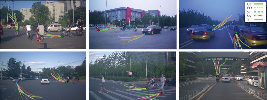
layer. gorithm computes a reasonably accurate predicted trajectoryFigure 5: Illustration of our TrafficPredict (TP) method on camera-based images. There are six scenarios with different road
conditions and traffic situations. We only show the trajectories of several instances in each scenario. The ground truth (GT) is
drawn in green and the prediction results of other methods (ED,SL,SA) are shown with different dashed lines. The prediction
trajectories of our TP algorithm (pink lines) are the closest to ground truth in most of the cases.
stance layer to capture the trajectories and interactions for
instances and use a category layer to summarize the simi-
larities of movement pattern of instances belong to the same
type and guide the prediction algorithm. All the information
in spatial and temporal space can be leveraged and trans-
ferred in our designed 4D Graph. Our method outperforms
previous state-of-the-art approaches in improving the accu-
racy of trajectory prediction on our new collected dataset for
heterogeneous traffic. We have evaluated our algorithm in
traffic datasets corresponding to urban dense scenarios and
observe good accuracy. Our algorithm is realtime and makes
(a) (b)
no assumption about the traffic conditions or the number of
Figure 6: Illustration of some prediction results by our agents.
method. The ground truth of trajectories of vehicles, bicy- Our approach has some limitations. Its accuracy varies
cles and pedestrians are drawn by blue, green and red re- based on traffic conditions and the duration of past trajec-
spectively. Predicted locations are all represented by yellow tories. In the future, we will consider more constraints, like
stars. For each instance, first five discrete points are observed the lane direction, the traffic signals and traffic rules, etc. to
positions, but there are some overlaps in the illustration of further improve the accuracy of trajectory prediction. Fur-
pedestrian trajectories. thermore, we would like to evaluate the performance in more
dense scenarios.
and is close to the ground truth. If we have prior trajectories
over a longer duration, the prediction accuracy increases. Acknowledgement
When traffic-agents are moving on straight lanes, it is easy
to predict their trajectories because almost all the traffic- Dinesh Manocha is supported in part by ARO Contract
agents are moving in straight direction. It is more chal- W911NF16-1-0085, and Intel. We appreciate all the people
lenging to provide accurate prediction in cross roads, as the who offered help for collecting the dataset.
agents are turning. Fig. 5 shows 2D experimental results of
two sequences in cross areas. There are some overlaps on References
trajectories. In these scenarios, there are many curves with [Administration 2005] U.S. Federal Highway Administration. Us
high curvature because of left turn. Our algorithm can com- highway 101 dataset. 2005. 3
pute accurate predicted trajectories in these cases. [Alahi et al. 2016] A. Alahi, K. Goel, V. Ramanathan, A. Robic-
quet, F.F. Li, and S. Savarese. Social lstm: Human trajectory pre-
diction in crowded spaces. In CVPR, pages 961–971, 2016. 2, 5,
Conclusion 6
In this paper, we have presented a novel LSTM-based algo- [Altché and Fortelle 2017] F. Altché and A. De La Fortelle. An lstm
rithm, TrafficPredict, for predicting trajectories for hetero- network for highway trajectory prediction. In ITSC, pages 353–
geneous traffic-agents in urban environment. We use a in- 359. IEEE, 2017. 2[Apolloscape 2018] Apolloscape. Trajectory dataset for urban traf- [Kalman 1960] R. E. Kalman. A new approach to linear filtering fic. 2018. http://apolloscape.auto/trajectory. and prediction problems. Journal of basic Engineering, 82(1):35– html. 5 45, 1960. 1, 2 [BaiduApollo 2018] BaiduApollo. 2018. https://github. [Khosroshahi 2017] A. Khosroshahi. Learning, Classification and com/ApolloAuto/apollo. 5 Prediction of Maneuvers of Surround Vehicles at Intersections us- [Bera et al. 2016] A. Bera, S. Kim, T. Randhavane, S. Pratapa, and ing LSTMs. PhD thesis, UC San Diego, 2017. 2 D. Manocha. Glmp-realtime pedestrian path prediction using [Kim et al. 2017] B. Kim, C.M. Kang, S.H. Lee, H. Chae, J. Kim, global and local movement patterns. In ICRA, pages 5528–5535. C.C. Chung, and J.W. Choi. Probabilistic vehicle trajectory predic- IEEE, 2016. 2 tion over occupancy grid map via recurrent neural network. ITSC, [Bera et al. 2017] A. Bera, T. Randhavane, and D. Manocha. Ag- 2017. 2 gressive, tense, or shy? identifying personality traits from crowd [Kingma and Ba 2014] D. Kingma and J. Ba. Adam: A method for videos. In IJCAI, volume 17, pages 112–118, 2017. 2 stochastic optimization. arXiv:1412.6980, 2014. 6 [Chandra et al. 2018a] R. Chandra, U. Bhattacharya, A. Bera, and [Lee et al. 2017] N. Lee, W. Choi, P. Vernaza, C.B. Choy, P.H. Torr, D. Manocha. Traphic: Trajectory prediction in dense and heteroge- and M. Chandraker. Desire: Distant future prediction in dynamic neous traffic using weighted interactions. arXiv:1812.04767, 2018. scenes with interacting agents. In CVPR, pages 336–345, 2017. 2 2 [Lefèvre et al. 2011] S. Lefèvre, C. Laugier, and J.Ibañez-Guzmán. [Chandra et al. 2018b] R. Chandra, T. Randhavane, U. Bhat- Exploiting map information for driver intention estimation at road tacharya, A. Bera, , and D. Manocha. Deeptagent: Realtime track- intersections. In IV, pages 583–588. IEEE, 2011. 2 ing of highly heterogeneous agents in very dense traffic. 2018. [Lerner et al. 2007] A. Lerner, Y. Chrysanthou, and D. Lischinski. http://gamma.cs.unc.edu/HTI/. 2 Crowds by example. In CGF, volume 26, pages 655–664. Wiley, [Cheung et al. 2018] E. Cheung, A. Bera, E. Kubin, K. Gray, and 2007. 3 Dinesh D. Manocha. Identifying driver behaviors using trajectory [Ma et al. 2017] Y. Ma, X. Zhu, Y. Sun, and B. Yan. Image tagging features for vehicle navigation. IROS, 2018. 2 by joint deep visual-semantic propagation. In Pacific Rim Confer- [Chung et al. 2015] J. Chung, K. Kastner, L. Dinh, K. Goel, A.C. ence on Multimedia, pages 25–35. Springer, 2017. 2 Courville, and Y. Bengio. A recurrent latent variable model for [Ma et al. 2018] Y. Ma, D. Manocha, and W. Wang. Autorvo: Local sequential data. In NIPS, pages 2980–2988, 2015. 2 navigation with dynamic constraints in dense heterogeneous traffic. [Cordts et al. 2016] M. Cordts, M. Omran, S. Ramos, T. Rehfeld, CSCS, 2018. 2 M. Enzweiler, R. Benenson, U. Franke, S. Roth, and B. Schiele. [Park et al. 2018] S. Park, B. Kim, C.M. Kang, C.C. Chung, and The cityscapes dataset for semantic urban scene understanding. In J.W. Choi. Sequence-to-sequence prediction of vehicle trajectory CVPR, pages 3213–3223, 2016. 3 via lstm encoder-decoder architecture. arXiv:1802.06338, 2018. 2 [Danielsson et al. 2007] S. Danielsson, L. Petersson, and A. Eide- [Pellegrini et al. 2009] S. Pellegrini, A. Ess, K. Schindler, and hall. Monte carlo based threat assessment: Analysis and improve- L. Van Gool. You’ll never walk alone: Modeling social behavior ments. In IV, pages 233–238. IEEE, 2007. 2 for multi-target tracking. In ICCV, pages 261–268. IEEE, 2009. 3, [Deo and Trivedi 2018] N. Deo and M.M. Trivedi. Multi-modal tra- 6 jectory prediction of surrounding vehicles with maneuver based [Rasmussen and Williams 2006] C.E. Rasmussen and C. K. lstms. arXiv:1805.05499, 2018. 2 Williams. Gaussian processes for machine learning. 2006. The [Firl et al. 2012] J. Firl, H. Stübing, S.A. Huss, and C. Stiller. Pre- MIT Press, Cambridge, MA, USA, 38:715–719, 2006. 1, 2 dictive maneuver evaluation for enhancement of car-to-x mobility [Toledo-Moreo and Zamora-Izquierdo 2009] R. Toledo-Moreo and data. In IV, pages 558–564. IEEE, 2012. 2 M.A. Zamora-Izquierdo. Imm-based lane-change prediction in [Geiger et al. 2013] A. Geiger, P. Lenz, C. Stiller, and R. Urtasun. highways with low-cost gps/ins. ITS, 10(1):180–185, 2009. 1 Vision meets robotics: The kitti dataset. IJRR, 32(11):1231–1237, [Treuille et al. 2006] A. Treuille, S. Cooper, and Z. Popović. Con- 2013. 3 tinuum crowds. TOG, 25(3):1160–1168, 2006. 2 [Goodfellow et al. 2016] I. Goodfellow, Y. Bengio, A. Courville, [Vaswani et al. 2017] A. Vaswani, N. Shazeer, N. Parmar, J. Uszko- and Y. Bengio. Deep learning, volume 1. MIT press Cambridge, reit, L. Jones, A.N. Gomez, Łukasz Kaiser, and Illia Polosukhin. 2016. 2 Attention is all you need. In NIPS, pages 5998–6008, 2017. 4 [Graves and Jaitly 2014] A. Graves and N. Jaitly. Towards end-to- [Vemula et al. 2017] A. Vemula, K. Muelling, and J. Oh. Social end speech recognition with recurrent neural networks. In ICML, attention: Modeling attention in human crowds. arXiv:1710.04689, pages 1764–1772, 2014. 2 2017. 2, 3, 4, 6 [Gupta et al. 2018] A. Gupta, J. Johnson, F.F. Li, S. Savarese, and [Vinyals et al. 2015] O. Vinyals, A. Toshev, S. Bengio, and D. Er- A. Alahi. Social gan: Socially acceptable trajectories with genera- han. Show and tell: A neural image caption generator. In CVPR, tive adversarial networks. In CVPR, number CONF, 2018. 2 pages 3156–3164, 2015. 2 [Helbing and Molnar 1995] D. Helbing and P. Molnar. Social force [Wang et al. 2008] J.M. Wang, D.J. Fleet, and A. Hertzmann. Gaus- model for pedestrian dynamics. Physical review E, 51(5):4282, sian process dynamical models for human motion. TPAMI, 1995. 2 30(2):283–298, 2008. 2 [Huang et al. 2018] X. Huang, X. Cheng, Q. Geng, B. Cao, [Yamaguchi et al. 2011] K. Yamaguchi, A.C. Berg, L.E. Ortiz, and D. Zhou, P. Wang, Y. Lin, and R. Yang. The apolloscape dataset T.L. Berg. Who are you with and where are you going? In CVPR, for autonomous driving. CVPR Workshop, 2018. 3 pages 1345–1352. IEEE, 2011. 2 [Jain et al. 2016] A. Jain, A.R. Zamir, S. Savarese, and A. Saxena. Structural-rnn: Deep learning on spatio-temporal graphs. In CVPR, pages 5308–5317, 2016. 3
You can also read