NEMO: NEURAL MESH MODELS OF CONTRASTIVE FEATURES FOR ROBUST 3D POSE ESTIMATION - OpenReview
←
→
Page content transcription
If your browser does not render page correctly, please read the page content below
Published as a conference paper at ICLR 2021

N E M O : N EURAL M ESH M ODELS OF C ONTRASTIVE
F EATURES FOR ROBUST 3D P OSE E STIMATION
 Angtian Wang, Adam Kortylewski, Alan Yuille
 Department of Computer Science
 Johns Hopkins University
 Maryland, MD 21218, USA
 {angtianwang, akortyl1, ayuille1}@jhu.edu

                                           A BSTRACT

         3D pose estimation is a challenging but important task in computer vision. In
         this work, we show that standard deep learning approaches to 3D pose estimation
         are not robust when objects are partially occluded or viewed from a previously
         unseen pose. Inspired by the robustness of generative vision models to partial
         occlusion, we propose to integrate deep neural networks with 3D generative rep-
         resentations of objects into a unified neural architecture that we term NeMo. In
         particular, NeMo learns a generative model of neural feature activations at each
         vertex on a dense 3D mesh. Using differentiable rendering we estimate the 3D
         object pose by minimizing the reconstruction error between NeMo and the feature
         representation of the target image. To avoid local optima in the reconstruction
         loss, we train the feature extractor to maximize the distance between the individ-
         ual feature representations on the mesh using contrastive learning. Our extensive
         experiments on PASCAL3D+, occluded-PASCAL3D+ and ObjectNet3D show
         that NeMo is much more robust to partial occlusion and unseen pose compared
         to standard deep networks, while retaining competitive performance on regular
         data. Interestingly, our experiments also show that NeMo performs reasonably
         well even when the mesh representation only crudely approximates the true ob-
         ject geometry with a cuboid, hence revealing that the detailed 3D geometry is
         not needed for accurate 3D pose estimation. The code is publicly available at
         https://github.com/Angtian/NeMo.

1   I NTRODUCTION
Object pose estimation is a fundamentally important task in computer vision with a multitude of real-
world applications, e.g. in self-driving cars, or partially autonomous surgical systems. Advances in
the architecture design of deep convolutional neural networks (DCNNs) Tulsiani & Malik (2015);
Su et al. (2015); Mousavian et al. (2017); Zhou et al. (2018) increased the performance of computer
vision systems at 3D pose estimation enormously. However, our experiment shows current 3D
pose estimation approaches are not robust to partial occlusion and when objects are viewed from
a previously unseen pose. This lack of robustness can have serious consequences in real-world
applications and therefore needs to be addressed by the research community.
In general, recent works follow either of two approaches for object pose estimation: Keypoint-based
approaches detect a sparse set of keypoints and subsequently align a 3D object representation to
the detection result. However, due to the sparsity of the keypoints, these approaches are highly
vulnerable when the keypoint detection result is affected by adverse viewing conditions, such as
partial occlusion. On the other hand, rendering-based approaches utilize a generative model, that is
built on a dense 3D mesh representation of an object. They estimate the object pose by reconstructing
the input image in a render-and-compare manner (Figure 1). While rendering-based approaches can
be more robust to partial occlusion Egger et al. (2018), their core limitation is that they model
objects in terms of image intensities. Therefore, they pay too much attention to object details that
are not relevant for the 3D pose estimation task. This makes them difficult to optimize Blanz &
Vetter (2003); Schönborn et al. (2017), and also requires a detailed mesh representation for every
shape variant of an object class (e.g. they need several types of sedan meshes instead of using one
prototypical type of sedan).

                                                 1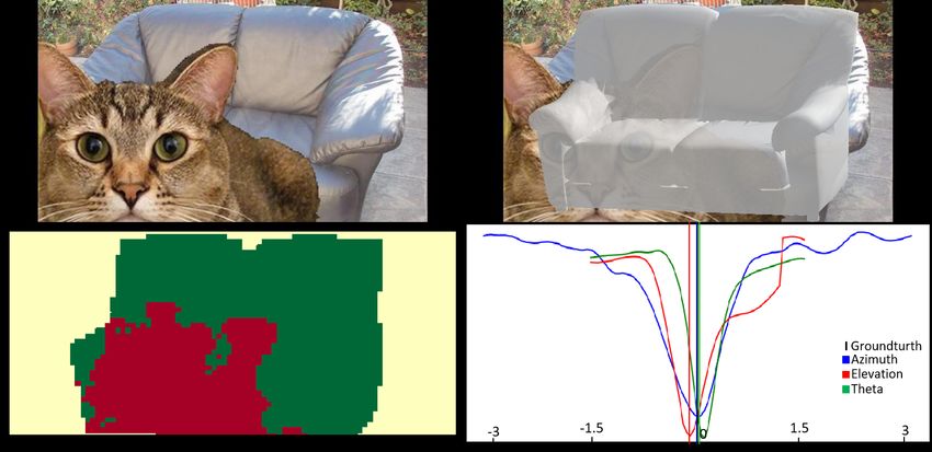
Published as a conference paper at ICLR 2021

                                                                 Vertex Feature Vectors
         CAD Model                                               Ɵ0
                            Render                               Ɵ1
                                                                 Ɵ2                                        Render
                                                                 Ɵ3
                                                                 Ɵ5
                                                                 Ɵ4
                                                                 …                                                     F
                                                                 Ɵr
                                                                                 Neural Mesh Model
                                                   Compare                                                              Compare
                                                                                                            CNN
                                                                                                          backbone

                                                                                                                       Fc

            Traditional Render-and-Compare: RGB Image                                     NeMo Render-and-Compare: Feature Map

Figure 1: Traditional render-and-compare approaches render RGB images and make pixel-level
comparisons. These are difficult to optimize due to the many local optima in the pixel-wise recon-
struction loss. In contrast, NeMo is a Neural Mesh Model that renders feature maps and compares
them with feature maps obtained via CNN backbone. The invariance of the neural features to nui-
sance variables, such as shape and color variations, enables a robust 3D pose estimation with simple
gradient-descent optimization of the neural reconstruction loss.

In this work, we introduce NeMo a rendering-based approach to 3D pose estimation that is highly
robust to partial occlusion, while also being able to generalize to previously unseen views. Our
key idea is to learn a generative model of an object category in terms of neural feature activations,
instead of image intensities (Figure 1). In particular, NeMo is composed of a prototypical mesh
representation of the object category and feature representations at each vertex of the mesh. The
feature representations are learned to be invariant to instance specific details (such as shape and
color variations) that are not relevant for the 3D pose estimation task. Specifically, we use contrastive
learning He et al. (2020); Wu et al. (2018); Bai et al. (2020) to ensure that the extracted features of an
object are distinct from each other (e.g. the features of the front tire of a car are different from those
of the back tire), while also being distinct from non-object features in the background. Furthermore,
we train a generative model of the feature activations at every vertex of the mesh representation.
During inference, NeMo estimates the object pose by reconstructing a target feature map with using
render-and-compare and gradient-based optimization w.r.t. the 3D object pose parameters.
We evaluate NeMo at 3D pose estimation on the PASCAL3D+ Xiang et al. (2014) and the Ob-
jectNet3D Xiang et al. (2016) dataset. Both datasets contain a variety of rigid objects and their
corresponding 3D CAD models. Our experimental results show that NeMo outperforms popular
approaches such as Starmap Zhou et al. (2018) at 3D pose estimation by a wide margin under par-
tial occlusion, and performs comparably when the objects are not occluded. Moreover, NeMo is
exceptionally robust when objects are seen from a viewpoint that is not present in the training data.
Interestingly, we also find that the mesh representation in NeMo can simply approximate the true
object geometry with a cuboid, and still perform very well. Our main contributions are:

      1. We propose a 3D neural mesh model of objects that is generative in terms of contrastive
         neural network features. This representation combines a prototypical geometric represen-
         tation of the object category with a generative model of neural network features that are
         invariant to irrelevant object details.
      2. We demonstrate that standard deep learning approaches to 3D pose estimation are highly
         sensitive to out-of-distribution data including partial occlusions and unseen poses. In con-
         trast, NeMo performs 3D pose estimation with exceptional robustness.
      3. In contrast to other rendering-based approaches that require instance-specific mesh repre-
         sentations of the target objects, we show that NeMo achieves a highly competitive 3D pose
         estimation performance even with a very crude prototypical approximation of the object
         geometry using a cuboid.

2    R ELATED W ORK
Category-Level Object Pose Estimation. Category-Level object pose estimation has been well
explored by the research community. A classical approach as proposes by Tulsiani & Malik (2015)
and Mousavian et al. (2017) was to formulate object pose estimation as a classification problem.
Another common category-level object pose estimation approach involves a two-step process Szeto
& Corso (2017); Pavlakos et al. (2017): First, semantic keypoints are detected interdependently and
subsequently a Perspective-n-Point problem is solved to find the optimal 3D pose of an object mesh

                                                             2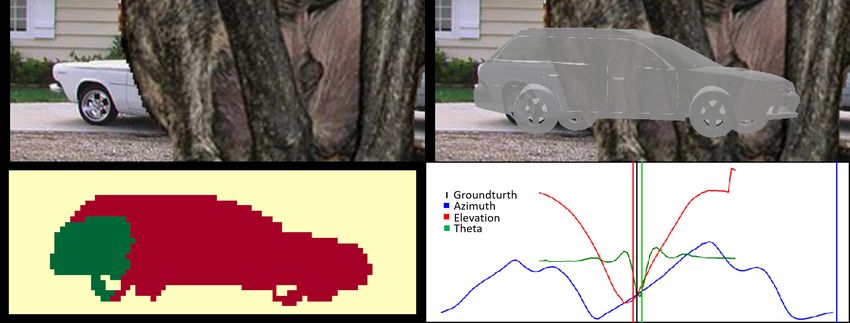
Published as a conference paper at ICLR 2021

Lu et al. (2000); Lepetit et al. (2009). Zhou et al. (2018) further improved this approach by utlizing
depth information. Recent work Wang et al. (2019); Chen et al. (2020) introduced render-and-
compare to for category-level pose estimation. However, both approaches used pixel-level image
synthesis and required detailed mesh models during training.In contrast, NeMo preforms render-
and-compare on the level of contrastive features, which are invariant to intra-category nuisances,
such as shape and color variations. This enables NeMo to achieve accurate 3D pose estimation
results even with a crude prototypical category-level mesh representation.
Pose Estimation under Partial Occlusion. Keypoint-based pose estimation methods are sensitive
to outliers, which can be caused by partial occlusion Pavlakos et al. (2017); Sundermeyer et al.
(2018). Some rendering-based approaches achieve satisfactory results on instance-level pose esti-
mation under partial occlusion Song et al. (2020); Peng et al. (2019); Zakharov et al. (2019); Li et al.
(2018). However, these approaches render RGB images or use instance-level constraints, e.g. pixel-
level voting, to estimate object pose. Therefore, these approaches are not suited for category-level
pose estimation. To the best of our knowledge, NeMo is the first approach that performs category-
level pose estimation robustly under partial occlusion.
Contrastive Feature Learning. Contrastive learning is widely used in deep learning research.
Hadsell et al. (2006) proposed an intuitive tuple loss, which was later extended to triplets and N-
Pair tuples Schroff et al. (2015); Sohn (2016). Recent contrastive learning approaches showed high
potential in unsupervised learning Wu et al. (2018); He et al. (2020). Oord et al. (2018); Han et al.
(2019) demonstrated the effectiveness of feature-level contrastive losses in representation learning.
Bai et al. (2020) proposed a keypoint detection framework by optimizing the feature representations
of keypoints with a contrastive loss. In this work, we use contrastive feature learning to encourage
the feature extraction backbone to extract locally distinct features. This, in turn, enables 3D pose
estimation by simply optimizing the neural reconstruction loss with gradient descent.
Robust Vision through Analysis-by-Synthesis. In a broader context, our work relates to a line of
work in the computer vision literature, which demonstrate that the explicit modeling of the object
structure significantly enhances the robustness of computer vision models, e.g. at 3D pose estimation
Zeeshan Zia et al. (2013), face reconstruction Egger et al. (2018) and human detection Girshick et al.
(2011) under occlusion. More specifically, our work builds on a recent line of work that introduced a
neural analysis-by-synthesis approach to vision Kortylewski et al. (2020b) and demonstrated its ef-
fectiveness in occlusion-robust image classification Kortylewski et al. (2020a;c) and object detection
Wang et al. (2020). Our work significantly extends neural analysis-by-synthesis to include an ex-
plicit 3D object representation, instead of 2D template-like object representations. This enables our
model to achieve state-of-the-art robustness at pose estimation through neural render-and-compare.

3     N E M O : A 3D GENERATIVE MODEL OF NEURAL FEATURES
We denote a feature representation of an input image I as Φ(I) = F l ∈ RH×W ×D . Where l is
the output of a layer l of a DCNN Φ, with D being the number of channels in layer l. fil ∈ RD is
a feaure vector in F l at position i on the 2D lattice P of the feature map. In the remainder of this
section we omit the superscript l for notational simplicity because this is fixed a-priori in our model.

3.1   N EURAL R ENDERING OF F EATURE M APS
Similar to other graphics-based generative models, such as e.g. 3D morphable models Blanz &
Vetter (1999); Egger et al. (2018), our model builds on a 3D mesh representation that is composed
of a set of 3D vertices Γ = {r ∈ R3 |r = 1, . . . , R}. For now, we assume the object mesh to be
given at training time but we will relax this assumption in later sections. Different from standard
graphics-based generative models, we do not store RGB values at each mesh vertex r but instead
store feature vectors Θ = {θr ∈ RD |r = 1, . . . , R}. Using standard rendering techniques, we can
use this 3D neural mesh model N = {Γ, Θ} to render feature maps:
                              F̄ (m) =
Published as a conference paper at ICLR 2021

class y by leveraging a 3D neural mesh representation Ny . Assuming that the 3D pose m of the
object in the input image is known, we define the likelihood of the feature representation F as:
                                           Y                  Y
                        p(F |Ny , m, B) =       p(fi |Ny , m)       p(fi0 |B).                   (2)
                                           i∈F G                 i0 ∈BG

The foreground FG is the set of all positions on the 2D lattice P of the feature map F that are
covered by the rendered neural mesh model. We compute FG by projecting the 3D vertices of the
mesh model Γy into the image using the ground truth camera pose m to obtain the 2D locations
of the visible vertices in the image FG = {st ∈ R2 |t = 1, . . . , T }. We define foreground feature
likelihoods to be Gaussian distributed:

                                           1            1
                          p(fi |Ny , m) = √ exp − 2 kfi − θr k2 .                                (3)
                                         σr 2π         2σr
Note that the correspondence between the feature vector fi in the feature map F and the vector θr
on the neural mesh model is given by the 2D projection of Ny with camera parameters m. Those
features that are not covered by the neural mesh model BG = P \ {F G}, i.e. are located in the
background, are modeled by a Gaussian likelihood:

                                         1            1             2
                           p(fi |B) =
                               0        √    exp − 2 kfi − βk ,
                                                             0                                (4)
                                       σ 2π          2σ
with mixture parameters B = {β, σ}.

3.3   T RAINING USING M AXIMUM L IKELIHOOD AND C ONTRASTIVE L EARNING

During training we want to optimize two objectives: 1) The parameters of the generative model as
defined in Equation 2 should be optimized to achieve maxmimum likelihood on the training data.
2) The backbone used for feature extraction ψ should be optimized to make the individual feature
vectors as disctinct from each other as possible.
Maximum likelihood estimation of the generative model. We optimize the parameters of the
generative model to minimize the negative log-likelihood of our model (Equation 2):
                  LM L (F, Ny , m, B) = − ln p(F |Ny , m, B)                                       (5)
                                           X  1               1
                                      =−         ln     √     − 2 kfi − θr k2                      (6)
                                                      σr 2π    2σr
                                          i∈F G

                                           X             1      1
                                        +         ln    √     − 2 kfi0 − βk2                       (7)
                                                       σ 2π    2σ
                                          i0 ∈BG

If we constrain the variances such that {σ 2 = σr2 = 1|∀r} then the maximum likelihood loss reduces
to:
                                               X                   X
                   LM L (F, Ny , m, B) = −C         kfi − θr k2 +      kfi0 − βk2 ,             (8)
                                              i∈F G                    i0 ∈BG

where C is a constant scalar.
Contrastive learning of the feature extractor. The general idea of the contrastive loss is to train
the feature extractor such that the individual feature vectors on the object are distinct from each
other, as well as from the background:
                                                  X       X
                          LF eature (F, FG) = −                 kfi − fi0 k2                    (9)
                                                   i∈F G i0 ∈F G\{i}
                                                   X X
                        LBack (F, FG, BG) = −                   kfi − fj k2 .                    (10)
                                                   i∈F G j∈BG

The contrastive feature loss LF eature encourages the features on the object to be distinct from each
other (e.g. the feature vectors at the front tire of a car are different from those of the back tire).
The contrastive background loss LBack encourages the features on the object to be distinct from the
features in the background. The overall loss used to train NeMo is:
        L(F, Ny , m, B) = LM L (F, Ny , m, B) + LF eature (F, FG) + LBack (F, FG, BG)            (11)

                                                   4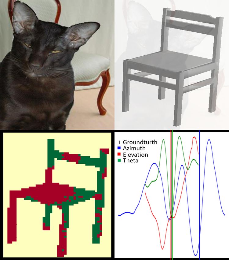
Published as a conference paper at ICLR 2021

                                                                                      Background Score Map
                                                                                                                              Loss Landscape
                                                   Clutter Feature β

                                                                                                                                               Groundturth
                                          CNN                                                                                                  Azimuth
                                        backbone                                      Occlusion Prediction Z                                   Elevation
                                                                                                                                               Theta

                                                            Fc                                                 FG
                                                                                                                    Loss
                                                                                                               BG
                                                                                                                           Final Pose Prediction
    Vertex Feature Vectors
    Ɵ0
    Ɵ1                                  Render
    Ɵ2
    Ɵ3
    Ɵ5
    Ɵ4
                                                             F
    …
    Ɵr
                    Neural Mesh Model                                                 Foreground Score Map
                                         m: camera parameter
                                                                       Backward

Figure 2: Overview of pose estimation: For each image, we use the trained CNN backbone to extract
feature map F . Meanwhile, using trained Neural Mesh Model and randomly initialized object pose,
we can render a feature map F̄ . By calculating similarity at each local of F and F̄ , we can create
a foreground score map, which demonstrate the object likelihood at each location. Similarly, we
can get a background score map via F and trained clutter model β. Using these two maps, we do
the occlusion inference to segment image into foreground region and background region. Then, we
calculate reconstruction loss and optimize object pose via minimize the loss. We also visualize the
loss landscape along all 3 object pose parameters, and the final pose prediction.
3.4       ROBUST 3D P OSE E STIMATION WITH R ENDER AND C OMPARE

After training the feature extractor and the generative model in NeMo, we apply the model for
estimating the camera pose parameters b. In particular we aim to optimize the model likelihood from
Equation 2 w.r.t. to the camera parameters in a render-and-compare manner. Following related work
on robust inference with generative models Kortylewski (2017); Egger et al. (2018) we optimize a
robust model likelihood:
                           Y                         z                    (1−zi )
                                                                                  Y
  p(F |Ny , m, B, zi ) =      [p(fi |Ny , m)p(zi =1)] i [p(fi |B)p(zi =0)]          p(fi0 |B). (12)
                                        i∈F G                                                                              i0 ∈BG

Here zi ∈ {0, 1} is a binary variable and p(zi =1) and p(zi =0) are the prior probabilities of the
respective values. Here zi is a binary variable that allows the background model p(fi |B) to explain
those locations in the feature map F that are in the foreground region FG, but which the foreground
model (fi |Ny , m) cannot explain well. A primary purpose of this mechanism is to make the cost
function robust to partial occlusion. Figure 2 illustrates the inference process. Given an initial
camera pose estimate we use the Neural Mesh Model to render a feature map F̄ and evaluate the re-
construction loss in the foreground region FG (foreground score map), as well as the reconstruction
error when using the background model only (background score map). Pixel-wised comparison of
foreground score and background score yield the occlusion map Z = {zi ∈ {0, 1}|∀i ∈ P}. The
map Z indicates where feature vectors are explained by either the foreground or background model.
A fundamental benefit of our Neural Mesh Models is that, they are generative on the level of neu-
ral feature activations. This makes the overall reconstruction loss very smooth compared to related
works who are generative on the pixel level. Therefore, NeMo can be optimized w.r.t. the pose
parameters with standard stochastic gradient descent. We visualize the loss as a function of the in-
dividual pose parameters in Figure 2. Note that the losses are generally very smooth and contain
one clear global optimum. This is in stark contrast to the optimization of classic generative models
at the level of RGB pixels, which often requires complex hand designed initialization and optimiza-
tion procedures to avoid the many local optima of the reconstruction loss Blanz & Vetter (2003);
Schönborn et al. (2017).

4        E XPERIMENT
We first describe the experimental setup in Section 4.1. Subsequently, we study the performance of
NeMo at 3D pose estimation in Section 4.2 and study the effect of crudely approximating the object
geometry within NeMo single 3d cuboid, that one cuboid represent all object in each category, and
multiple 3d cuboid, that one cuboid represent only one subtype of object in each category. We ablate
the important modules of our model in Section 4.4.

4.1       E XPERIMENTAL S ETUP

Evaluation. The task of 3D object pose estimation involves the prediction of three rotation pa-
rameters (azimuth, elevation, in-plane rotation) of an object relative to the camera. In our eval-

                                                                                  5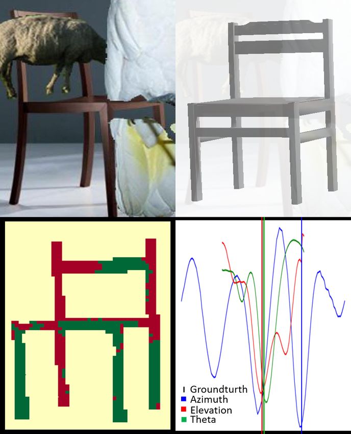
Published as a conference paper at ICLR 2021
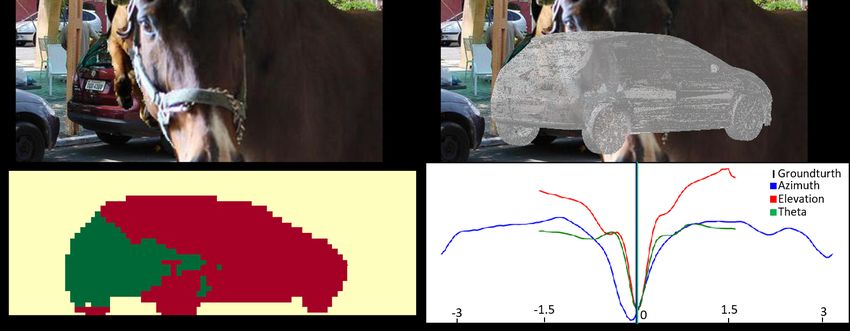
(a) Aeroplane, L0 (b) Bus, L1
(c) Sofa, L2 (d) Car, L3
Figure 3: Qualitative results of NeMo on PASCAL3D+ (L0) and occluded PASCAL3D+ (L1 &
L2 & L3) for different categories under different occlusion level. For each example, we show four
subfigures. Top-left: the input image; Top-right: A mesh superimposed on the input image in the
predicted 3D pose. Bottom-left: The occluder localization result, where yellow is background, green
is the non-occluded area of the object and red is the occluded area as predicted by NeMo. Bottom-
right: The loss landscape for each individual camera parameter respectively. The colored vertical
lines demonstrate the final prediction and the ground-truth parameter is at center of x-axis.
uation, we follow the protocol as proposed in related work Zhou et al. (2018) to measure the
pose estimation error between the predicted rotation matrix and the ground truth rotation matrix:
klog m(R√T
pred Rgt )kF
∆ (Rpred , Rgt ) = 2
. We report two commonly used evaluation metrics the me-
dian of the rotation error, the percentage of predicted angles within a given accuracy threshold.
Specifically, we use the thresholds pi pi
6 and 18 . Following Zhou et al. (2018), we assume the centers
and scales of the objects are given in all experiments.
Datasets. We evaluate NeMo on both the PASCAL3D+ dataset Xiang et al. (2014) and the occluded
PASCAL3D+ dataset Wang et al. (2020). PASCAL3D+ contains 12 man-made object categories
with 3D pose annotations and 3D meshes for each category respectively. We follow Wang et al.
(2020) and Bai et al. (2020) to split the PASCAL3D+ into a training set with 11045 images and
validation set with 10812 images. The occluded PASCAL3D+ dataset is a benchmark to evalu-
ate robustness under occlusion. This dataset simulates realistic man-made occlusion by artificially
superimposing occluders collected from the MS-COCO dataset Lin et al. (2014) on objects in PAS-
CAL3D+. The dataset contains all 12 classes of objects from PASCAL3D+ dataset with three levels
of occlusion, where L1: 20-40%, L2: 40-60%, L3: 60-80% of the object area are occluded.
We further test NeMo on the ObjectNet3D dataset Xiang et al. (2016), which is also a category-level
3D pose estimation benchmark. ObjectNet3D contains 100 different categories with 3D meshes,
it contains totally 17101 training samples and 19604 testing samples, including 3556 occluded or
truncated testing samples. Following Zhou et al. (2018), we report pose estimation results on 18 cat-
egories. Note that different from StarMap, we use all images during evaluation, including occluded
or truncated samples.
Training Setup. In the training process, we use the 3D meshes (see Section 4.2 for experiments
without the mesh geometry), the locations and scales of objects, and the 3D poses. We use Blender
Community (2018) to reduce the resolution of the mesh because the meshes provided in PAS-
CAL3D+ have a very high number of vertices. In order to balance the performance and compu-
tational cost, in particular the cost of the rendering process, we limit the size of the feature map
produced by backbone to 18 of the input image. To achieve this, we use the ResNet50 with two
additional upsample layers as our backbone. We train a backbone for each category separately, and
learn a Neural Mesh Model for each subtype in a category. We follow hyperparameter settings from
Bai et al. (2020) for the contrastive loss. We train NeMo for 800 training epochs with a batch size
of 108, which takes around 3 to 5 hours to train a category using 6 NVIDIA RTX Titan GPUs.
Baselines. We compare our model to StarMap Zhou et al. (2018) using their official implementation
and training setup. Following common practice, we also evaluate a popular baseline that formu-
6
Published as a conference paper at ICLR 2021

Table 1: Pose estimation results on PASCAL3D+ and the occluded PASCAL3D+ dataset. Occlusion
level L0 are the orignal images from PASCAL3D+, while Occlusion Level L1 to L3 are the occluded
PASCAL3D+ images with increasing occlusion ratio. We evaluate both baseline and NeMo using
Accuracy (percentage, higher better) and Median Error (degree, lower better). Note that NeMo is
exceptionally robust to partial occlusion.

   Evaluation Metric             ACC π6 ↑                       π ↑
                                                           ACC 18                    MedErr ↓
   Occlusion Level         L0     L1 L2       L3     L0     L1 L2       L3     L0     L1 L2       L3
   Res50-General          88.1   70.4 52.8   37.8   44.6   25.3 14.5    6.7   11.7   17.9 30.4   46.4
   Res50-Specific         87.6   73.2 58.4   43.1   43.9   28.1 18.6    9.9   11.8   17.3 26.1   44.0
   StarMap                89.4   71.1 47.2   22.9   59.5   34.4 13.9    3.7    9.0   17.6 34.1   63.0
   NeMo                   84.1   73.1 59.9   41.3   60.4   45.1 30.2   14.5    9.3   15.6 24.1   41.8
   NeMo-MultiCuboid       86.7   77.2 65.2   47.1   63.2   49.9 34.5   17.8    8.2   13.0 20.2   36.1
   NeMo-SingleCuboid      86.1   76.0 63.9   46.8   61.0   46.3 32.0   17.1    8.8   13.6 20.9   36.5

lates pose estimation as a classification problem. In particular, we evaluate the performance of a
deep neural network classifier that uses the same backbone as NeMo. We train a category specific
Resnet50 (Res50-Specific), which formulates the pose estimation in each category as an individual
classification problem. Furthermore, we train a non-specific Resnet50 (Res50-General), which per-
forms pose estimation for all categories in a single classification task. We report the result of both
architectures using the implementation provided by Zhou et al. (2018).
Inference via Feature-level Rendering. We implement the NeMo inference pipeline (see 3.4)
using PyTorch3D Ravi et al. (2020). Specifically, we render the Neural Mesh Models into feature
map F̄ using the feature representations Θ stored at each mesh vertex. We estimate the object
pose by minimizing the reconstruction loss as introduced in Equation 12. For initialization of pose
optimization, we uniformly sample 144 different poses (12 azimuth angles, 4 elevation angles, 3
in-plane rotations respectively). Then we pick the initial pose with minimum reconstruction loss
as a starting point of optimization (optimization conduct with only the chosen pose, others will be
deprecated). On average each image takes about 8s with a single GPU for inference. The whole
inference process on PASCAL3D+ takes about 3 hours using a 8 GPU machine.

4.2   ROBUST 3D P OSE E STIMATION U NDER O CCLUSION

Baseline performances. Table 1 (for categories specific scores, see 6) illustrates the 3D pose es-
timation results on PASCAL3D+ under different levels of occlusion. In the low accuracy setting
(ACC π6 ) StarMap performs exceptionally well when the object is non-occluded (L0). However,
with increasing level of partial occlusion, the performance of StarMap degrades massively, falling
even below the basic classification models Res50-General and Res50-Specific. These results high-
light that today’s most common deep networks for 3D pose estimation are not robust. Similar,
generalization patterns can be observed for the high accuracy setting (ACC 18π ). However, we can

observe that the classification baselines do not perform as well as before, and hence are not well
suited for fine-grained 3D pose estimation. Nevertheless, they outperform StarMap at high occlu-
sion levels (L2 & L3).
NeMo. We evaluate NeMo in three different setups: NeMo uses a down-sampled object mesh as
geometry representation, NeMo-MultiCuboid and NeMo-SingleCuboid approximate the 3D object
geometry crudely using 3D cuboid boxes. We discuss the cuboid generation and results in detail
in the next paragraph. Compared to the baseline performances, we observe that NeMo achieves
competitive performance at estimating the 3D pose of non-occluded objects. Moreover, NeMo is
much more robust compared to all baseline approaches. In particular, we observe that NeMo
achieves the highest performance at every evaluation metric when the objects are partially occluded.
Note that the training data for all models is exactly the same.
To further investigate and understand the robustness of NeMo, we qualitatively analyze the pose
estimation and occluder location predictions of NeMo in Figure 3. Each subfigure shows the input
image, the pose estimation result, the occluder localization map and the loss as a function of the
pose angles. We visualize the loss landscape along each pose parameter (azimuth, elevation and
in-plane rotation) by sampling the individual parameters in a fixed step size, while keeping all other
parameters at their ground-truth value. We further split the binary occlusion map Z into three regions
to highlight the occluder localization performance of NeMo. In particular, we split the region that
is explained by the background model into a yellow and a red region. The red region is covered by
rendered mesh and highlights the locations with the projected region of the mesh, which the neural

                                                    7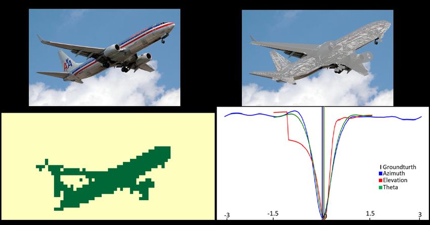
Published as a conference paper at ICLR 2021

Table 2: Pose estimation results of ObjectNet3D. Evaluated via pose estimation accuracy percentage
for error under π6 (higher better). Both baseline and NeMo evaluated on all images of given category,
including occluded and truncated. Overall, NeMo has higher accuracy in 14 categories while lower
in 4 categories.

ACC π6 ↑            bed    bookshelf calculator cellphone computer cabinet       guitar   iron   knife
StarMap             40.0     72.9       21.1       41.9     62.1    79.9          38.7     2.0    6.1
NeMo-MultiCuboid    56.1     53.7       57.1       28.2     78.8    83.6          38.8    32.3    9.8
ACC π6 ↑         microwave    pen       pot        rifle   slipper stove         toilet    tub wheelchair
StarMap             86.9     12.4       45.1        3.0     13.3    79.7          35.6    46.4   17.7
NeMo-MultiCuboid    90.3      3.7       66.7       13.7      6.1    85.2          74.5    61.6   71.7
Table 3: Pose estimation results on PASCAL3D+ for objects in seen and unseen poses. The his-
togram on the left shows how we separate the PASCAL3D+ test dataset into subsets based on the
azimuth pose of the object. We have similarly split the training dataset and trained all models only
on the ”seen” subset. We evaluate on both test sets (Seen & Unseen). Note the strong generalization
performance of NeMo in unseen view points.

                       Evaluation Metric        ACC π6 ↑              π ↑
                                                                  ACC 18             MedErr ↓
                       Data Split             Seen Unseen       Seen Unseen       Seen Unseen
                       Res50-General          91.7    37.2      47.9    5.3       10.8    45.8
                       Res50-Specific         91.2    34.7      47.9    4.0       10.8    48.5
                       StarMap                93.1    49.8      68.6   13.5        7.3    36.0
                       NeMo-MultiCuboid       88.6    54.7      70.2   31.0        6.6    34.9
                       NeMo-SingleCuboid      88.5    54.3      68.6   27.9        7.0    35.1

mesh model cannot explain well. Hence these mark the locations in the image that NeMo predicts
to be occluded. From the qualitative illustrations, we observe that NeMo maintains high robustness
even under extreme occlusion, when only a small part of the object is visible. Furthermore, we can
clearly see that NeMo can approximately localize the occluders. This occluder localization property
of NeMo makes our model not just more robust but also much more human-interpretable compared
to standard deep network approaches.
NeMo without detailed object mesh. We approximate the object geometry in NeMo by replacing
the downsampled mesh with 3D cuboid boxes (see Figure 5). The vertices of the cuboid meshes
are evenly distributed on all six sides of the cuboid. For generating the cuboids, we use three con-
straint: 1) The cuboid should cover all the vertices of the original mesh with minimum volume;
2) The distances between each pair of adjacent vertices should be similar; 3) The total number of
vertices for each mesh should be around 1200 vertices. We generate two different types of models.
NeMo-MultiCuboid uses a separate cuboid for each object mesh in an object category, while NeMo-
SingleCuboid uses on cuboid for all instances of a category.
We report the pose estimations results with NeMo using cuboid meshes in Table 1. The results show
that approximating the detailed mesh representations of a category with a single 3D cuboid gives
surprisingly good results. In particular, NeMo-SingleCuboid even often outperforms our standard
model. This shows that generative models of neural network feature activations must not retain the
detailed object geometry, because the feature activations are invariant to detailed shape properties.
Moreover, NeMo-MultiCube outperforms the SingleCube model significantly. This suggests that
for some categories the size between different sub-types can be very differnt (e.g. for the airplane
class it could be a passanger jet or a fighter jet). Therefore, a single mesh may not be representative
enough for some object categories. The MultiCuboid model even outperforms our the model with
detailed mesh geometry. This is very likely caused by difficulties during the down-sampling of the
original meshes in PASCAL3D+, which might remove important parts of the object geometry.
We also conduct experiment on ObjectNet3D dataset, which reported in Table 2. The result demon-
strates that NeMo outperforms StarMap in 14 categories out of all 18 categories. Note that due to
the considerable number of occluded and truncated images in ObjectNet3D dataset, this dataset is
significantly harder than PASCAL3D+, however, NeMo still demonstrates reasonable accuracy.

4.3   G ENERALIZATION TO U NSEEN V IEWS

To further investigate robustness of NeMo to out-of-distribution data, we evaluate the performance
of NeMo when objects are observed from previously unseen viewpoints. For this, we split the
PASCAL3D+ dataset into two sets based on the ground-truth azimuth angle. In particular, we use

                                                  8
Published as a conference paper at ICLR 2021

Table 4: Ablation study on PASCAL3D+ and occluded PASCAL3D+. All ablation experiments are
conducted with the NeMo-MultiCuboid model. The performance is reported in terms of Accuracy
(percentage, higher better) and Median Error (degree, lower better).

    Evaluation Metric             ACC π6 ↑                       π ↑
                                                            ACC 18                    MedErr ↓
    Occlusion Level         L0     L1 L2       L3     L0     L1 L2       L3     L0     L1 L2       L3
    NeMo                   86.7   77.3 65.2   47.1   63.2   49.2 34.5   17.8   8.2    13.1 20.2   36.1
    NeMo w/o outlier       85.2   76.0 63.2   44.4   61.8   47.9 32.4   16.2   8.5    13.5 20.7   41.6
    NeMo w/o contrastive   69.7   58.0 44.6   26.9   40.8   27.7 14.7    5.6   18.3   27.7 37.0   61.0
Table 5: Sensitivity of NeMo-MultiCuboid under different numbers of pose initializations during
inference (Init Samples) on PASCAL3D+.

                           Init Samples ACC π6 ↑ ACC 18
                                                     π ↑ MedErr ↓

                             144(Std.)   86.7     63.2      8.2
                                 72      86.3     63.0      8.3
                                 36      84.1     61.1      8.8
                                 12      81.2     57.7      9.3
                                  6      80.4     57.7      9.6
                                  1      54.9     38.9     35.6

the front and rear views for training. We evaluate all approaches on the full testing set and split the
performance into seen (front and rear) and unseen (side) poses. The histogram on the left of Table
4 shows the distribution of ground-truth azimuth angles in the PASCAL3D+ test dataset. The seen-
test-set contains 7305 images while the unseen-test-set contains 3507 images. Table 4 shows that
NeMo can significantly better generalize to novel viewpoints compared to the baselines. For some
categories the accuracy of NeMo on the unseen-test-set is even comparable to seen-test-set (Table 7).
These results highlight the importance of building neural networks with 3D internal representations,
which enable them to generalize exceptionally well to unseen 3D transformations.

4.4    A BLATION S TUDY

In Table 4, we study the effect of each individual module of NeMo. Specifically, we remove the
clutter feature, background score and occluder prediction during inference, and only use foreground
score to calculate pose loss. This reduces the robustness to occlusion significantly. Furthermore, we
remove the contrastive loss and use neural features that were extracted with an ImageNet-pretrained
Resnet50 with non-parametric-upsampling. This leads to a massive decrease in performance, and
hence highlights the importance of learning locally distinct feature representations. Table 5 (and
Table 10) study the sensitivity of NeMo to the random pose initialization before the pose optimiza-
tion. In this ablation, we evaluate NeMo-MultiCuiboid with 144 down to 1 uniformly sampled
initialization poses. Note that we do not run 144 optimization processes. We instead evaluate the
reconstruction error for each initialization and start the optimization from the initializaiton with the
lowest error. Hence, every experiment only involves one optimization run. The results demonstrate
that NeMo benefits from the smooth lose landscape. With 6 initial samples NeMo achieves a rea-
sonable performance, while 72 initial poses almost yield the maximum performance. This ablation
clearly highlights that, unlike standard Render-and-Compare approaches Blanz & Vetter (1999);
Schönborn et al. (2017), NeMo does not require complex designed initialization strategies.

5     C ONCLUSION

In this work, we considered the problem of robust 3D pose estimation with neural networks. We
found that standard deep learning approaches do not give robust predictions when objects are
partially occluded or viewed from an unseen pose. In an effort to resolve this fundamental limitation
we developed Neural Mesh Models (NeMo), a neural network architecture that integrates a pro-
totypical mesh representation with a generative model of neural features. We combine NeMo
with contrastive learning and show that this makes possible to estimate the 3D pose with very high
robustness to out-of-distribution data using simple gradient-based render-and-compare. Our ex-
periments demonstrate the superiority of NeMo compared to related work on a range of challenging
datasets.

                                                     9
Published as a conference paper at ICLR 2021

ACKNOWLEDGMENTS
We gratefully acknowledge funding support from ONR N00014-18-1-2119, ONR N00014-20-1-
2206, the Institute for Assured Autonomy at JHU with Grant IAA 80052272, and the Swiss National
Science Foundation with Grant P2BSP2.181713. We also thank Weichao Qiu, Qing Liu, Yutong Bai
and Jiteng Mu for suggestions on our paper.

R EFERENCES
Yutong Bai, Angtian Wang, Adam Kortylewski, and Alan Yuille. Coke: Localized contrastive
  learning for robust keypoint detection. arXiv preprint arXiv:2009.14115, 2020. 2, 3, 6

Volker Blanz and Thomas Vetter. A morphable model for the synthesis of 3d faces. In Proceedings
  of the 26th annual conference on Computer graphics and interactive techniques, pp. 187–194,
  1999. 3, 9

Volker Blanz and Thomas Vetter. Face recognition based on fitting a 3d morphable model. IEEE
  Transactions on pattern analysis and machine intelligence, 25(9):1063–1074, 2003. 1, 5

Xu Chen, Zijian Dong, Jie Song, Andreas Geiger, and Otmar Hilliges. Category level object pose
  estimation via neural analysis-by-synthesis. arXiv preprint arXiv:2008.08145, 2020. 3

Blender Online Community. Blender - a 3D modelling and rendering package. Blender Foundation,
  Stichting Blender Foundation, Amsterdam, 2018. URL http://www.blender.org. 6

Bernhard Egger, Sandro Schönborn, Andreas Schneider, Adam Kortylewski, Andreas Morel-
  Forster, Clemens Blumer, and Thomas Vetter. Occlusion-aware 3d morphable models and an
  illumination prior for face image analysis. International Journal of Computer Vision, 126(12):
  1269–1287, 2018. 1, 3, 5

Ross Girshick, Pedro Felzenszwalb, and David McAllester. Object detection with grammar models.
  Advances in Neural Information Processing Systems, 24:442–450, 2011. 3

Raia Hadsell, Sumit Chopra, and Yann LeCun. Dimensionality reduction by learning an invariant
  mapping. In 2006 IEEE Computer Society Conference on Computer Vision and Pattern Recogni-
  tion (CVPR’06), volume 2, pp. 1735–1742. IEEE, 2006. 3

Tengda Han, Weidi Xie, and Andrew Zisserman. Video representation learning by dense predictive
  coding. In Proceedings of the IEEE International Conference on Computer Vision Workshops,
  pp. 0–0, 2019. 3

Kaiming He, Haoqi Fan, Yuxin Wu, Saining Xie, and Ross Girshick. Momentum contrast for
  unsupervised visual representation learning. In Proceedings of the IEEE/CVF Conference on
  Computer Vision and Pattern Recognition, pp. 9729–9738, 2020. 2, 3

Adam Kortylewski. Model-based image analysis for forensic shoe print recognition. PhD thesis,
  University of Basel, 2017. 5

Adam Kortylewski, Ju He, Qing Liu, and Alan L Yuille. Compositional convolutional neural net-
  works: A deep architecture with innate robustness to partial occlusion. In Proceedings of the
  IEEE/CVF Conference on Computer Vision and Pattern Recognition, pp. 8940–8949, 2020a. 3

Adam Kortylewski, Qing Liu, Angtian Wang, Yihong Sun, and Alan Yuille. Compositional convolu-
  tional neural networks: A robust and interpretable model for object recognition under occlusion.
  International Journal of Computer Vision, pp. 1–25, 2020b. 3

Adam Kortylewski, Qing Liu, Huiyu Wang, Zhishuai Zhang, and Alan Yuille. Combining composi-
  tional models and deep networks for robust object classification under occlusion. In Proceedings
  of the IEEE/CVF Winter Conference on Applications of Computer Vision, pp. 1333–1341, 2020c.
  3

Vincent Lepetit, Francesc Moreno-Noguer, and Pascal Fua. Epnp: An accurate o (n) solution to the
  pnp problem. International journal of computer vision, 81(2):155, 2009. 3

                                               10
Published as a conference paper at ICLR 2021
Yi Li, Gu Wang, Xiangyang Ji, Yu Xiang, and Dieter Fox. Deepim: Deep iterative matching for 6d
pose estimation. In Proceedings of the European Conference on Computer Vision (ECCV), pp.
683–698, 2018. 3
Tsung-Yi Lin, Michael Maire, Serge Belongie, James Hays, Pietro Perona, Deva Ramanan, Piotr
Dollár, and C Lawrence Zitnick. Microsoft coco: Common objects in context. In European
conference on computer vision, pp. 740–755. Springer, 2014. 6
C-P Lu, Gregory D Hager, and Eric Mjolsness. Fast and globally convergent pose estimation from
video images. IEEE transactions on pattern analysis and machine intelligence, 22(6):610–622,
2000. 3
Arsalan Mousavian, Dragomir Anguelov, John Flynn, and Jana Kosecka. 3d bounding box esti-
mation using deep learning and geometry. In Proceedings of the IEEE Conference on Computer
Vision and Pattern Recognition, pp. 7074–7082, 2017. 1, 2
Aaron van den Oord, Yazhe Li, and Oriol Vinyals. Representation learning with contrastive predic-
tive coding. arXiv preprint arXiv:1807.03748, 2018. 3
Georgios Pavlakos, Xiaowei Zhou, Aaron Chan, Konstantinos G Derpanis, and Kostas Daniilidis.
6-dof object pose from semantic keypoints. In 2017 IEEE international conference on robotics
and automation (ICRA), pp. 2011–2018. IEEE, 2017. 2, 3
Sida Peng, Yuan Liu, Qixing Huang, Xiaowei Zhou, and Hujun Bao. Pvnet: Pixel-wise voting
network for 6dof pose estimation. In Proceedings of the IEEE Conference on Computer Vision
and Pattern Recognition, pp. 4561–4570, 2019. 3
Nikhila Ravi, Jeremy Reizenstein, David Novotny, Taylor Gordon, Wan-Yen Lo, Justin Johnson,
and Georgia Gkioxari. Accelerating 3d deep learning with pytorch3d. arXiv:2007.08501, 2020.
7
Sandro Schönborn, Bernhard Egger, Andreas Morel-Forster, and Thomas Vetter. Markov chain
monte carlo for automated face image analysis. International Journal of Computer Vision, 123
(2):160–183, 2017. 1, 5, 9
Florian Schroff, Dmitry Kalenichenko, and James Philbin. Facenet: A unified embedding for face
recognition and clustering. In Proceedings of the IEEE conference on computer vision and pattern
recognition, pp. 815–823, 2015. 3
Kihyuk Sohn. Improved deep metric learning with multi-class n-pair loss objective. In Advances in
neural information processing systems, pp. 1857–1865, 2016. 3
Chen Song, Jiaru Song, and Qixing Huang. Hybridpose: 6d object pose estimation under hybrid
representations. In Proceedings of the IEEE/CVF Conference on Computer Vision and Pattern
Recognition (CVPR), June 2020. 3
Hao Su, Charles R Qi, Yangyan Li, and Leonidas J Guibas. Render for cnn: Viewpoint estima-
tion in images using cnns trained with rendered 3d model views. In Proceedings of the IEEE
International Conference on Computer Vision, pp. 2686–2694, 2015. 1
Martin Sundermeyer, Zoltan-Csaba Marton, Maximilian Durner, Manuel Brucker, and Rudolph
Triebel. Implicit 3d orientation learning for 6d object detection from rgb images. In Proceed-
ings of the European Conference on Computer Vision (ECCV), pp. 699–715, 2018. 3
Ryan Szeto and Jason J Corso. Click here: Human-localized keypoints as guidance for viewpoint
estimation. In Proceedings of the IEEE International Conference on Computer Vision, pp. 1595–
1604, 2017. 2
Shubham Tulsiani and Jitendra Malik. Viewpoints and keypoints. In Proceedings of the IEEE
Conference on Computer Vision and Pattern Recognition, pp. 1510–1519, 2015. 1, 2
Angtian Wang, Yihong Sun, Adam Kortylewski, and Alan L. Yuille. Robust object detection under
occlusion with context-aware compositionalnets. In Proceedings of the IEEE/CVF Conference on
Computer Vision and Pattern Recognition (CVPR), June 2020. 3, 6
11Published as a conference paper at ICLR 2021
He Wang, Srinath Sridhar, Jingwei Huang, Julien Valentin, Shuran Song, and Leonidas J Guibas.
Normalized object coordinate space for category-level 6d object pose and size estimation. In
Proceedings of the IEEE Conference on Computer Vision and Pattern Recognition, pp. 2642–
2651, 2019. 3
Zhirong Wu, Yuanjun Xiong, Stella X Yu, and Dahua Lin. Unsupervised feature learning via non-
parametric instance discrimination. In Proceedings of the IEEE Conference on Computer Vision
and Pattern Recognition, pp. 3733–3742, 2018. 2, 3
Yu Xiang, Roozbeh Mottaghi, and Silvio Savarese. Beyond pascal: A benchmark for 3d object
detection in the wild. In IEEE Winter Conference on Applications of Computer Vision (WACV),
2014. 2, 6
Yu Xiang, Wonhui Kim, Wei Chen, Jingwei Ji, Christopher Choy, Hao Su, Roozbeh Mottaghi,
Leonidas Guibas, and Silvio Savarese. Objectnet3d: A large scale database for 3d object recog-
nition. In European Conference Computer Vision (ECCV), 2016. 2, 6
Sergey Zakharov, Ivan Shugurov, and Slobodan Ilic. Dpod: 6d pose object detector and refiner. In
Proceedings of the IEEE International Conference on Computer Vision, pp. 1941–1950, 2019. 3
M Zeeshan Zia, Michael Stark, and Konrad Schindler. Explicit occlusion modeling for 3d object
class representations. In Proceedings of the IEEE Conference on Computer Vision and Pattern
Recognition, pp. 3326–3333, 2013. 3
Xingyi Zhou, Arjun Karpur, Linjie Luo, and Qixing Huang. Starmap for category-agnostic key-
point and viewpoint estimation. In Proceedings of the European Conference on Computer Vision
(ECCV), pp. 318–334, 2018. 1, 2, 3, 6, 7
12Published as a conference paper at ICLR 2021
A A PPENDIX
Table 6: Pose estimation results on PASCAL3D+ (L0) for all categories respectively. Results re-
ported in Accuracy (percentage, higher better) and Median Error (degree, lower better).
aero bike boat bottle bus car chair table mbike sofa train tv Mean
↑ ACC π6 Res50-General 83.0 79.6 73.1 87.9 96.8 95.5 91.1 82.0 80.7 97.0 94.9 83.3 88.1
↑ ACC π6 Res50-Specific 79.5 75.8 73.5 90.3 93.5 95.6 89.1 82.4 79.7 96.3 96.0 84.6 87.6
↑ ACC π6 StarMap 85.5 84.4 65.0 93.0 98.0 97.8 94.4 82.7 85.3 97.5 93.8 89.4 89.4
↑ ACC π6 NeMo 73.3 66.4 65.5 83.0 87.4 98.8 82.8 81.9 74.6 94.7 87.0 85.5 84.1
↑ ACC π6 NeMo-MultiCuboid 76.9 82.2 66.5 87.1 93.0 98.0 90.1 80.5 81.8 96.0 89.3 87.1 86.7
↑ ACC π6 NeMo-SingleCuboid 82.2 78.4 68.1 88.0 91.7 98.2 87.0 76.9 85.0 95.0 83.0 82.2 86.1
↑ ACC 18
π Res50-General 31.3 25.7 23.9 35.9 67.2 63.5 37.0 40.2 18.9 62.5 51.2 24.9 44.6
↑ ACC 18
π Res50-Specific 29.1 22.9 25.3 39.0 62.7 62.9 37.5 42.0 19.5 57.5 50.2 25.4 43.9
↑ ACC 18
π StarMap 49.8 34.2 25.4 56.8 90.3 81.9 67.1 57.5 27.7 70.3 69.7 40.0 59.5
↑ ACC 18
π NeMo 39.0 31.3 29.6 38.6 83.1 94.8 46.9 58.1 29.3 61.1 71.1 66.4 60.4
↑ ACC 18
π NeMo-MultiCuboid 43.1 35.3 36.4 48.6 89.7 95.5 49.5 56.5 33.8 68.8 75.9 56.8 63.2
↑ ACC 18
π NeMo-SingleCuboid 49.7 29.5 37.7 49.3 89.3 94.7 49.5 52.9 29.0 58.5 70.1 42.4 61.0
↓ MedErr Res50-General 13.3 15.9 15.6 12.1 8.9 8.8 11.5 11.4 16.6 8.7 9.9 15.8 11.7
↓ MedErr Res50-Specific 14.2 17.3 15.4 11.7 9.0 8.8 12.0 11.0 17.1 9.2 10.0 14.9 11.8
↓ MedErr StarMap 10.0 14.0 19.7 8.8 3.2 4.2 6.9 8.5 14.5 6.8 6.7 12.1 9.0
↓ MedErr NeMo 13.8 17.5 18.3 12.8 3.4 2.7 10.7 8.2 16.1 8.0 5.6 6.6 9.3
↓ MedErr NeMo-MultiCuboid 11.8 13.4 14.8 10.2 2.6 2.8 10.1 8.8 14.0 7.0 5.0 8.1 8.2
↓ MedErr NeMo-SingleCuboid 10.1 16.3 14.9 10.2 3.2 3.2 10.1 9.3 14.1 8.6 5.4 12.2 8.8
Table 7: Pose estimation results on occluded PASCAL3D+ occlusion L1 for all categories respec-
tively. Results reported in Accuracy (percentage, higher better) and Median Error (degree, lower
better).
aero bike boat bottle bus car chair table mbike sofa train tv Mean
↑ ACC π6 Res50-General 57.3 56.8 51.4 78.3 82.5 80.0 62.3 63.1 61.1 84.9 87.8 69.8 70.4
↑ ACC π6 Res50-Specific 54.0 59.5 48.9 84.4 86.1 84.4 67.1 64.9 65.9 87.8 92.4 74.5 73.2
↑ ACC π6 StarMap 52.6 65.3 42.0 81.8 87.9 86.1 64.5 66.5 62.8 76.9 85.2 59.7 71.1
↑ ACC π6 NeMo 49.0 51.4 52.9 73.5 82.2 94.3 70.2 67.9 53.8 86.7 75.0 79.4 73.1
↑ ACC π6 NeMo-MultiCuboid 58.1 68.8 53.4 78.8 86.9 94.0 76.0 70.0 61.8 87.3 82.8 82.8 77.2
↑ ACC π6 NeMo-SingleCuboid 61.9 63.4 52.9 81.3 84.8 92.7 78.4 68.2 68.9 87.1 80.3 76.9 76.0
↑ ACC 18
π Res50-General 11.8 12.5 12.3 26.5 45.0 40.7 14.7 22.3 10.7 24.4 34.9 13.0 25.3
↑ ACC 18
π Res50-Specific 12.4 10.7 13.8 30.2 46.9 44.8 21.2 24.0 10.4 28.0 40.6 17.9 28.1
↑ ACC 18
π StarMap 15.6 15.1 10.8 36.2 66.6 58.1 26.6 32.0 14.4 23.8 47.4 13.0 34.4
↑ ACC 18
π NeMo 18.5 19.9 19.1 24.0 72.1 82.0 25.8 35.7 12.6 44.3 54.0 49.0 45.1
↑ ACC 18
π NeMo-MultiCuboid 25.4 23.3 22.9 36.7 86.9 84.8 33.1 36.8 20.8 46.5 61.0 46.3 49.9
↑ ACC 18
π NeMo-SingleCuboid 29.3 18.0 24.3 41.5 76.1 80.5 27.2 31.4 19.4 39.9 55.1 32.0 46.3
↓ MedErr Res50-General 25.3 24.5 29.0 14.9 10.6 11.2 22.4 18.1 23.3 15.5 11.7 21.1 17.9
↓ MedErr Res50-Specific 26.8 23.7 31.0 13.8 10.5 10.6 18.2 16.7 21.8 13.6 10.9 19.3 17.3
↓ MedErr StarMap 27.3 22.1 38.9 12.9 7.0 8.2 19.1 17.2 21.7 16.8 10.6 24.1 17.6
↓ MedErr NeMo 30.8 29.0 27.3 17.6 5.9 5.1 18.6 14.7 27.4 11.3 8.8 10.2 15.6
↓ MedErr NeMo-MultiCuboid 22.6 18.6 25.8 14.1 4.7 4.6 15.1 13.8 21.2 11.0 8.0 11.3 13.0
↓ MedErr NeMo-SingleCuboid 18.9 23.2 26.7 12.6 5.2 5.4 15.6 15.4 20.1 12.1 8.6 15.3 13.6
13Published as a conference paper at ICLR 2021
Table 8: Pose estimation results on occluded PASCAL3D+ occlusion L2 for all categories respec-
tively. Results reported in Accuracy (percentage, higher better) and Median Error (degree, lower
better).
aero bike boat bottle bus car chair table mbike sofa train tv Mean
↑ ACC π6 Res50-General 33.3 40.2 33.6 70.6 69.5 57.0 41.8 47.4 43.3 66.8 80.4 58.1 52.8
↑ ACC π6 Res50-Specific 36.3 44.9 36.1 76.1 73.1 65.5 53.2 49.5 45.4 72.7 88.3 65.0 58.4
↑ ACC π6 StarMap 28.5 38.9 21.3 65.0 61.7 59.3 37.5 44.7 43.2 55.1 56.4 36.2 47.2
↑ ACC π6 NeMo 38.2 41.2 39.6 58.3 72.6 84.7 50.7 51.1 34.9 70.1 60.0 64.6 59.9
↑ ACC π6 NeMo-MultiCuboid 43.1 55.7 43.3 69.1 79.8 84.5 58.8 58.4 43.9 76.4 64.3 70.3 65.2
↑ ACC π6 NeMo-SingleCuboid 43.4 49.6 43.6 76.0 71.2 83.8 61.9 55.9 50.9 78.3 63.1 68.6 63.9
↑ ACC 18
π Res50-General 6.1 4.5 7.2 20.1 25.9 21.4 9.5 13.2 6.1 14.0 23.0 8.6 14.5
↑ ACC 18
π Res50-Specific 5.7 6.9 8.0 25.5 33.9 29.1 13.0 11.6 6.8 18.4 32.0 13.8 18.6
↑ ACC 18
π StarMap 3.8 5.8 2.4 19.7 30.5 24.5 7.7 9.6 5.1 9.6 21.5 5.8 13.9
↑ ACC 18
π NeMo 10.7 10.5 11.3 13.9 55.8 60.6 9.3 20.3 6.3 26.1 34.6 32.1 30.2
↑ ACC 18
π NeMo-MultiCuboid 12.8 16.6 16.8 21.9 62.3 64.6 17.2 20.3 12.3 32.4 38.2 32.7 34.5
↑ ACC 18
π NeMo-SingleCuboid 14.9 11.1 15.6 18.2 56.0 62.4 17.4 18.7 10.2 30.5 36.4 22.4 32.0
↓ MedErr Res50-General 49.3 42.5 58.5 17.7 15.9 21.3 35.4 32.0 36.1 20.3 15.2 25.3 30.4
↓ MedErr Res50-Specific 45.8 33.9 52.8 16.3 12.4 15.1 27.1 30.9 32.4 18.3 12.3 24.1 26.1
↓ MedErr StarMap 55.2 37.1 69.1 20.6 19.0 21.3 39.2 34.0 35.5 27.0 24.8 40.3 34.1
↓ MedErr NeMo 39.8 37.7 44.2 24.8 8.8 7.7 29.7 28.5 47.5 16.9 18.2 17.0 24.1
↓ MedErr NeMo-MultiCuboid 38.5 26.4 38.2 18.8 7.0 7.3 23.0 23.0 36.0 14.0 14.9 16.1 20.2
↓ MedErr NeMo-SingleCuboid 39.9 30.6 38.8 19.5 8.3 7.8 21.3 24.8 29.5 14.2 16.9 18.5 20.9
Table 9: Pose estimation results on occluded PASCAL3D+ occlusion L3 for all categories respec-
tively. Results reported in Accuracy (percentage, higher better) and Median Error (degree, lower
better).
aero bike boat bottle bus car chair table mbike sofa train tv Mean
↑ ACC π6 Res50-General 18.3 20.8 21.2 62.1 57.0 36.9 31.1 32.2 24.3 56.2 64.5 53.4 37.8
↑ ACC π6 Res50-Specific 20.0 33.4 25.5 67.5 57.8 42.0 40.7 33.9 30.3 56.6 82.8 56.5 43.1
↑ ACC π6 StarMap 7.6 18.5 10.6 46.3 35.1 25.3 22.5 24.6 15.9 26.4 24.0 19.5 22.9
↑ ACC π6 NeMo 24.0 31.3 27.4 43.3 48.8 62.8 31.8 29.7 18.4 44.2 34.5 51.4 41.3
↑ ACC π6 NeMo-MultiCuboid 23.8 34.3 29.5 53.9 56.0 65.5 43.4 41.5 25.4 58.2 43.2 54.1 47.1
↑ ACC π6 NeMo-SingleCuboid 20.6 33.8 27.6 61.7 49.9 61.8 44.7 41.2 35.3 62.9 47.9 50.2 46.8
↑ ACC 18
π Res50-General 1.6 2.3 2.9 11.9 14.4 7.6 3.8 5.7 3.1 7.9 12.7 8.9 6.7
↑ ACC 18
π Res50-Specific 2.0 5.5 4.8 16.7 21.1 13.1 5.9 5.7 4.3 9.9 22.5 6.0 9.9
↑ ACC 18
π StarMap 0.8 1.7 1.1 11.8 8.3 4.8 2.1 2.6 1.6 2.8 5.2 0.7 3.7
↑ ACC 18
π NeMo 4.4 6.2 6.7 6.8 26.5 31.1 3.4 6.7 2.0 9.3 13.0 16.7 14.5
↑ ACC 18
π NeMo-MultiCuboid 5.5 5.2 7.9 10.8 34.2 37.4 7.4 8.2 4.5 15.8 15.1 15.9 17.8
↑ ACC 18
π NeMo-SingleCuboid 4.7 6.7 8.6 11.7 29.2 33.7 11.0 10.7 4.9 17.8 17.2 10.9 17.1
↓ MedErr Res50-General 69.8 70.9 73.2 22.7 24.9 46.7 41.5 44.4 59.8 26.3 21.3 28.4 46.4
↓ MedErr Res50-Specific 65.8 47.1 75.8 20.9 18.5 46.6 35.9 49.9 56.3 26.4 15.3 26.5 44.0
↓ MedErr StarMap 87.0 67.6 90.2 32.6 51.3 64.0 60.7 53.2 73.4 51.0 52.7 54.7 63.0
↓ MedErr NeMo 65.3 48.4 65.2 34.5 34.9 17.2 44.6 55.7 74.3 33.7 47.6 29.3 41.8
↓ MedErr NeMo-MultiCuboid 69.8 49.6 63.0 28.2 19.4 14.9 35.4 39.9 60.0 23.7 38.1 27.2 36.1
↓ MedErr NeMo-SingleCuboid 74.8 46.1 70.1 24.5 30.2 16.3 35.2 37.5 50.5 21.5 31.7 29.9 36.5
14Published as a conference paper at ICLR 2021
Table 10: Full table for 5. This table shows category specific results of NeMo-MultiCuboid pose
estimation performance on PASCAL3D+ using different number of initialization pose during in-
ference. The Init Samples shows total number of initialization pose e.g. 144 means we uniformly
sample 12(azimuth) * 4(elevation) * 3(in-plane rotation) poses. Std. mean this setting is standard
settings and used in main experiment.
Category aero bike boat bottle bus car chair table mbike sofa train tv Mean
144(Std.) 76.9 82.2 66.5 87.1 93.0 98.0 90.1 80.5 81.8 96.0 89.3 87.1 86.7
72 77.1 81.9 64.6 86.5 93.0 98.0 89.2 81.3 82.2 95.8 85.9 87.0 86.3
36 74.6 79.2 60.0 86.6 89.8 94.7 88.6 79.5 80.0 95.2 86.4 86.5 84.1
↑ ACC π6
12 73.4 78.1 57.1 86.2 79.9 86.9 90.1 81.6 79.3 94.6 82.5 86.5 81.2
6 69.7 78.1 58.3 85.7 82.5 90.9 87.8 68.6 80.3 95.0 79.4 86.0 80.4
1 38.7 33.6 34.2 86.9 54.9 40.6 77.5 68.3 27.8 89.7 78.6 84.7 54.9
144(Std.) 43.1 35.3 36.4 48.6 89.7 95.5 49.5 56.5 33.8 68.8 75.9 56.8 63.2
72 43.2 35.7 36.6 47.5 89.8 95.2 48.7 56.7 34.0 69.1 72.6 56.6 63.0
36 41.3 33.2 31.6 47.8 85.5 91.8 49.5 56.1 33.0 68.4 74.1 56.3 61.1
↑ ACC 18
π
12 41.1 32.2 26.6 47.3 73.3 84.4 49.7 57.0 33.5 67.9 67.6 55.8 57.7
6 38.3 32.1 30.5 46.9 78.4 88.2 48.1 46.7 33.0 68.1 66.9 55.5 57.7
1 22.7 19.7 21.6 47.4 44.7 37.9 44.6 47.3 14.6 65.5 62.1 54.5 38.9
144(Std.) 11.8 13.4 14.8 10.2 2.6 2.8 10.1 8.8 14.0 7.0 5.0 8.1 8.2
72 11.9 13.4 15.7 10.4 2.6 2.8 10.3 8.7 14.0 7.0 5.2 8.2 8.3
36 12.4 14.5 19.1 10.4 2.8 2.9 10.1 8.8 14.2 7.0 5.0 8.2 8.8
↓ MedErr
12 12.5 14.8 22.6 10.5 3.8 3.1 10.0 8.7 14.5 7.1 5.7 8.3 9.3
6 14.2 14.8 21.4 10.5 3.1 2.9 10.4 11.5 14.3 7.1 5.6 8.4 9.6
1 49.0 77.0 63.9 10.4 27.7 43.6 11.1 11.3 78.0 7.4 6.0 8.7 35.6
Table 11: Experiment for NeMo-MultiCuboid when subtype is not given during inference. In the
w/o subtype experiment we use NMMs of all subtypes to do inference on each image respectively,
then pick the predicted pose with subtypes with minimum reconstruction loss. The result demon-
strate that distinguishing subtypes is not necessary for pose estimation with NeMo.
↑ ACC π6 aero bike boat bottle bus car chair table mbike sofa train tv Mean
with subtype 76.9 82.2 66.5 87.1 93.0 98.0 90.1 80.5 81.8 96.0 89.3 87.1 86.7
L0
w/o subtype 77.7 78.3 70.9 82.6 94.5 98.7 86.4 75.5 83.7 93.8 89.3 81.0 85.8
with subtype 58.1 68.8 53.4 78.8 86.9 94.0 76.0 70.0 61.8 87.3 82.8 82.8 77.2
L1
w/o subtype 59.4 63.4 56.0 74.9 90.3 96.1 73.4 63.0 64.7 83.8 84.0 77.6 76.5
with subtype 43.1 55.7 43.3 69.1 79.8 84.5 58.8 58.4 43.9 76.4 64.3 70.3 65.2
L2
w/o subtype 46.3 48.1 44.3 67.3 84.0 86.2 61.5 50.9 45.1 70.2 67.0 67.4 64.7
with subtype 23.8 34.3 29.5 53.9 56.0 65.5 43.4 41.5 25.4 58.2 43.2 54.1 47.1
L3
w/o subtype 26.1 28.6 31.5 54.9 61.2 66.9 44.3 34.4 25.0 54.0 49.2 53.8 47.2
15Published as a conference paper at ICLR 2021
Original Mesh Models
Original Mesh Model Down Sampled Mesh
Cuboid for All Subtypes
(a) DownSample
Original Mesh Model Cuboid for Each Subtype
(b) MultiCuboid (c) SingleCuboid
Figure 5: Using detailed mesh model we can create all type of mesh models for NeMo. (a) We
use remesh method in Blender to down sample the original mesh. The processed mesh contains
1722 vertices. (b) Following rules in 4.2, we create subtype specificed cuboid (one cuboid for each
subtype), which used in NeMo-MultiCuboid approach. The cuboid contains 1096 vertices. (c) We
create the subtype general cuboid by requiring the cuboid cover original meshes of all subtypes.
And we use the created cuboid to represent all objects in this category, which reported as NeMo-
SingleCuboid. This cuboid contains 1080 vertices.
16Published as a conference paper at ICLR 2021
(a) Chair, L2 (b) Car, L3
(d) Diningtable, L1
(c) Chair, L2
Figure 6: Visualization of failure case of NeMo on occluded PASCAL3D+. For each example, we
show four subfigures. Top-left: the input image; Top-right: A mesh superimposed on the input
image in the predicted 3D pose. Bottom-left: The occluder localization result, where yellow is
background, green is the non-occluded area of the object and red is the occluded area as predicted
by NeMo. Bottom-right: The loss landscape for each individual camera parameter respectively. The
colored vertical lines demonstrate the final prediction and the ground-truth parameter is at center of
x-axis.
Table 12: Pose estimation results on PASCAL3D+ under unseen pose for CAR category. Figure
shows the distribution of azimuth in PASCAL3D+ testing set of car category and our splitting.
Evaluation Metric ACC π6 ↑ π ↑
ACC 18 ↓ MedErr ↓
Data Split Seen Unseen Seen Unseen Seen Unseen
Res50-General 97.2 55.3 72.2 11.5 8.1 25.5
Res50-Specific 97.2 52.5 70.5 11.7 8.2 27.7
StarMap 98.2 77.6 93.7 34.2 3.4 15.5
NeMo-MultiCuboid 96.8 97.0 94.8 85.4 2.6 5.2
NeMo-SingleCuboid 98.0 97.8 96.3 78.8 2.9 5.9
17You can also read