Testing constant absolute and relative ambiguity aversion
←
→
Page content transcription
If your browser does not render page correctly, please read the page content below
Available online at www.sciencedirect.com

                                           ScienceDirect
                                Journal of Economic Theory 181 (2019) 309–332
                                                                                           www.elsevier.com/locate/jet

        Testing constant absolute and relative ambiguity
                           aversion ✩
                               Aurélien Baillon a , Lætitia Placido b,∗
a Erasmus School of Economics, Erasmus University Rotterdam, P.O. Box 1738, Rotterdam, 3000 DR, the Netherlands
    b Department of Economics and Finance, Baruch College, City University of New York, Bernard Baruch Way,
                                              New York, NY 10010, USA
            Received 10 April 2017; final version received 13 December 2018; accepted 16 February 2019
                                          Available online 27 February 2019

Abstract
   Recent applications have demonstrated the crucial role of decreasing absolute ambiguity aversion in
financial and saving decisions. Yet, most ambiguity models predict that ambiguity aversion remains constant
when individuals become better off overall. We propose the first tests of constant absolute and relative
ambiguity aversion, using simple variations of the Ellsberg paradoxes. Our tests are axiomatically founded
and grounded in the theoretical literature. We implemented these tests in an experiment. Our results call for
the use of ambiguity models that can accommodate decreasing aversion toward ambiguity.
© 2019 The Authors. Published by Elsevier Inc. This is an open access article under the CC BY license
(http://creativecommons.org/licenses/by/4.0/).

JEL classification: C91; D81

Keywords: Ambiguity aversion; Ellsberg; CARA; CRRA; Ambiguity models

   Does ambiguity attitude change when individuals become better off overall? Addressing
risk attitude, seminal papers in finance from the 1960s and 1970s explained portfolio alloca-
tions by hypothesizing that absolute risk aversion is decreasing but relative risk aversion is
increasing (see in particular Arrow, 1971). Recently, several papers developing applications of

 ✩
    We thank Han Bleichrodt, Marciano Siniscalchi, and the audience at RUD 2015 in Milano for helpful comments on
this paper. The research of Aurélien Baillon was made possible by a grant of the Netherlands Organization for Scientific
Research (452-13-013).
 * Corresponding author.
    E-mail address: laetitia.placido@baruch.cuny.edu (L. Placido).

https://doi.org/10.1016/j.jet.2019.02.006
0022-0531/© 2019 The Authors. Published by Elsevier Inc. This is an open access article under the CC BY license
(http://creativecommons.org/licenses/by/4.0/).
310 A. Baillon, L. Placido / Journal of Economic Theory 181 (2019) 309–332
Klibanoff et al.’s (2005) smooth ambiguity model demonstrated the crucial role of decreasing
absolute ambiguity aversion (DAAA) on saving behavior (Berger, 2014; Osaki and Schlesinger,
2013; Gierlinger and Gollier, 2014) and prevention behavior (Berger, 2016) and in the survival
of ambiguity-averse agents in a market with expected utility agents (Guerdjikova and Sci-
ubba, 2015). At odds with these applications, most ambiguity models assume constant absolute
ambiguity aversion (CAAA), and some predict constant relative ambiguity aversion (CRAA).
In particular, CAAA is implied by Gilboa and Schmeidler’s (1989) maxmin expected utility,
Schmeidler’s (1989) Choquet expected utility, Ghirardato et al.’s (2004) invariant biseparable
preferences and alpha-maxmin expected utility, Maccheroni et al.’s (2006) variational prefer-
ences, Siniscalchi’s (2009) vector expected utility and Grant and Polak’s (2013) mean dispersion
preferences. CRAA is implied by Gilboa and Schmeidler’s (1989) maxmin expected utility and
Chateauneuf and Faro’s (2009) confidence preferences. Klibanoff et al.’s (2005) can accommo-
date either CAAA (with an exponential function) or CRAA (with a power function).
We propose the first tests of CAAA and CRAA using simple variations of the Ellsberg para-
doxes (Ellsberg, 1961). Our tests are axiomatically founded and grounded in the theoretical
literature. Consider an urn containing ten red balls and ten balls that are yellow or green in
unknown proportion. A decision maker is indifferent between winning a prize if he draws a yel-
low ball from the urn and winning the same prize with probability p. He is now told that he can
win the prize not only if the ball drawn is yellow but also if it is red. Hence, irrespective of his
prior(s) about the probability of winning, his chances increase by 12 . CAAA predicts that the de-
cision maker should be indifferent between betting on yellow or red and winning with probability
p + 12 . This prediction provides a simple test of CAAA.1
Consider again the initial bet on yellow and imagine that the red balls are removed from
the urn. Irrespective of the number of yellow balls, the chance of drawing one of them is now
multiplied by 2 with respect to the initial bet on yellow. In other words, regardless of what
the decision maker’s prior(s) was (were) about the probability of drawing a yellow ball, this
probability has doubled. The decision maker exhibits CRAA if he is indifferent between betting
on yellow in the urn without red balls and winning with probability p × 2.2
We conducted an experiment implementing these and similar tests of absolute and relative risk
aversion. At the aggregate level, our results support decreasing absolute and relative ambiguity
aversion. At the individual level, although CAAA is a reasonable assumption for about 40%
of the subjects, we find that a very similar proportion of subjects exhibit DAAA. Almost half
of the subjects also satisfied DRAA. Studying the magnitude of the deviations from constant
absolute and relative ambiguity aversion, our results suggest that CAAA would not make accurate
predictions for most subjects unless we accept errors of up to 10%. Our findings encourage
theoretical and empirical applications of ambiguity to rely on models accounting for decreasing
aversion toward ambiguity.
So far, we have discussed how ambiguity attitude evolves when the decision maker becomes
better off in terms of utility. Alternatively, one may want to predict changes in ambiguity attitude
1 Consider a maxmin expected utility maximizer, who has a set of priors in mind and evaluates a bet by the lowest
expected utility he may get. If he thinks there may be between 3 and 7 yellow balls, then his initial winning probability
is between 0.15 and 0.35. He will be indifferent between the bet on yellow and a bet on p = 0.15 (the worst case). When
he can also win with red, his winning probability now belongs to [0.65, 0.85] and he is now indifferent between the new
bet and winning with probability p + 12 = 0.65.
2 The maxmin expected utility maximizer of footnote 1 now has in mind a probability between 0.30 and 0.70, and will
be indifferent between betting on yellow and p × 2 = 0.30.A. Baillon, L. Placido / Journal of Economic Theory 181 (2019) 309–332 311
when the decision maker becomes better off in terms of wealth. This approach requires to account
for risk attitudes, as shown by Cerreia-Vioglio et al. (2017). If utility is linear, then our results
remain: a CAAA decision maker will display the same preferences irrespective of whether he
faces a change in wealth or in utility. If the decision maker is risk averse and satisfies expected
utility, then his preferences will remain unchanged at higher wealth levels if he is CARA and
CRAA (Cerreia-Vioglio et al., 2017, see 1.3 for further details). Combining our results about risk
and ambiguity, we demonstrate that an increase of wealth can have mixed effects on ambiguity
aversion.
The following section formally introduces our tests of CAAA and CRAA. Section 2 describes
the experiment, and the results are reported in section 3. Section 4 concludes.
1. Conceptual background
1.1. Absolute and relative risk aversion
We briefly recall the definitions of constant, decreasing, and increasing absolute risk aversion
(referred to as CARA, DARA, and IARA) and their relative counterparts (CRRA, DRRA, and
IRRA). Risk attitude can be characterized by comparing how much an agent values a lottery with
the expected value of the lottery. Let M = [0, m], an interval of the reals, represent all possible
outcomes. We denote by L the set of all finite lotteries over M. The binary lottery xp y yields
x with probability p and y otherwise. The outcome z such that z ∼ is called the certainty
equivalent (CE) of and is denoted ce(). Risk aversion holds if ce() ≤ E() with E() being
the expected value of . CARA [DARA, IARA] is characterized by
ce ( + W ) = [≥, ≤] ce() + W (1.1)
where + W is obtained by adding W > 0 to all outcomes of (assuming + W ∈ L). CRRA
[DRRA, IRRA] is defined by
ce(α) = [≤, ≥] αce() (1.2)
where α is obtained by multiplying all outcomes of by α ∈ (0, 1).
1.2. Absolute and relative ambiguity aversion
Just as CEs are useful to characterize risk attitude, probability equivalents (PEs) are key to
study ambiguity attitude (Dimmock et al., 2016).3 In the following, we show how to characterize
constant, decreasing, and increasing absolute ambiguity aversion (CAAA, DAAA, and IAAA)
and their relative counterparts (CRAA, DRAA, and IRAA).
Uncertainty is introduced through a state space S, which is a finite set of states of nature
s. As usual in the Anscombe and Aumann (1963) framework, an act f maps S to the set of
lotteries L. An act yielding the same lottery for all s ∈ S is referred to as the lottery itself. F is
the set of all acts. The decision maker has preferences over F . The mixture αf + (1 − α) g is
the act that assigns the lottery αf (s) + (1 − α) g (s) to s ∈ S. Let = m1 0 and = m0 0 be the
best and the worst lotteries. We say that preferences satisfy monotonicity if f (s) being first-order
stochastically dominated by lottery for all s implies f .
3 PEs are also often called matching probabilities.312 A. Baillon, L. Placido / Journal of Economic Theory 181 (2019) 309–332
Consider the lottery mp 0 such that f ∼ mp 0. If we scale the utility over M between 0 and 1,
virtually all ambiguity models interpret p as the utility of act f . We call such p the probability
equivalent of f and denote it pe(f ). If f is such that f (s) = mps 0, we define the complementary
act f c of f by f c (s) = m1−ps 0.4
Schmeidler’s (1989) defined ambiguity aversion as follows: for all f, g ∈ F and α ∈ (0, 1),
f ∼ g implies αf + (1 − α)g f . This definition implies Siniscalchi’s (2009, axiom 10) comple-
mentary ambiguity aversion, which states that, in our notation, f ∼ mpe(f ) 0 and f c ∼ mpe(f c ) 0
imply 12 f + 12 f c m 1 pe(f )+ 1 pe(f c ) 0. Using 12 f + 12 f c = m 1 0, and assuming that preferences
2 2 2
over lotteries satisfy first-order stochastic dominance, complementary ambiguity aversion im-
plies pe(f ) + pe(f c ) ≤ 1. Hence, comparing the sum of the probability equivalents of two
complementary acts with 1 is a test of complementary ambiguity aversion and of stronger
ambiguity-aversion conditions.
We use the definition of CAAA proposed by Grant and Polak (2013):
Definition 1 (CAAA). For all act f in F , lotteries 1 , 2 , and 3 , and α ∈ (0, 1), αf +(1 − α) 1
α2 + (1 − α) 1 ⇒ αf + (1 − α) 3 α2 + (1 − α) 3 .
Grant and Polak (2013) showed that this condition is a weakening of Schmeidler’s (1989)
comonotonic independence, Gilboa and Schmeidler’s (1989) certainty independence, and Mac-
cheroni et al.’s (2006) weak certainty independence.5 All these axioms require invariance to
translations of utility profiles. Hence, all ambiguity models relying on one of these axioms and
listed in the introduction predict constant absolute aversion toward ambiguity. In terms of PEs
and using the best and the worst lotteries, CAAA can be tested with the condition:
pe(αf + (1 − α) ) = pe(αf + (1 − α) ) + (1 − α) (1.3)
with α ∈ (0, 1). In words, increasing the probability of obtaining the best outcome m by (1 − α)
for all states of nature increases the PE by (1 − α).
Observation 1. Assume that preferences satisfy weak ordering and monotonicity. Then CAAA
implies Eq. (1.3).
Proof. Assume pe(αf + (1 − α) ) = p, that is αf + (1 − α) ∼ mp 0. Any f must yield
lotteries that are (weakly) dominated by getting the best outcome for sure and therefore, act
αf + (1 − α) yields lotteries that are (weakly) first-order stochastically dominated by mα 0.
Hence, p ≤ α (by monotonicity) and we can define 2 = m p 0. We thus have αf + (1 − α) ∼
α
α2 + (1 − α) . Then CAAA implies αf + (1 − α) ∼ α2 + (1 − α) = mp+1−α 0. 2
Observation 2. Gilboa and Schmeidler’s (1989) maxmin expected utility, Schmeidler’s (1989)
Choquet expected utility, Ghirardato et al.’s (2004) invariant biseparable preferences and
alpha-maxmin expected utility, Maccheroni et al.’s (2006) variational preferences, Siniscalchi’s
(2009) vector expected utility and Grant and Polak’s (2013) mean dispersion preferences imply
Eq. (1.3).
4 The pair f, f c is complementary according to definition 3 of Siniscalchi (2009).
5 Trautmann and Wakker (2018) showed that these axioms were violated because ambiguity attitude changes between
gains ans losses.A. Baillon, L. Placido / Journal of Economic Theory 181 (2019) 309–332 313
Proof. Grant and Polak (2013) showed that all these models imply CAAA. Furthermore, they
all assume weak ordering and monotonicity. Hence, by Observation 1, these models imply
Eq. (1.3). 2
We will further classify decision makers as DAAA [IAAA] using:
pe(αf + (1 − α) ) ≥ [≤] pe(αf + (1 − α) ) + (1 − α) (1.4)
with α ∈ (0, 1). Under the same assumptions as before, the conditions for DAAA and IAAA are
implications of recent definitions proposed by Chambers et al. (2014, Definition 9). The DAAA
condition is also implied by an axiom used by Ghirardato and Siniscalchi (2015) and Xue (2018,
Axiom A.2.1).
Maxmin expected utility (Gilboa and Schmeidler, 1989) is invariant to shifts of utility profiles
but also to multiplication or rescaling. Its core axiom, certainty independence, implies CAAA and
Chateauneuf and Faro’s (2009) worst independence axiom, a form of homotheticity or invariance
to mixture with the worst lottery. We propose to use this latter axiom to define CRAA because it
is similar to CRRA (the only type of homothetic preferences under expected utility).
Definition 2 (CRAA). For all acts f, g in F , and α ∈ (0, 1), f ∼ g ⇒ αf + (1 − α) ∼ αg +
(1 − α).
In terms of PEs, we can observe CRAA by
pe(αf + (1 − α) ) = αpe(f ) (1.5)
with α ∈ (0, 1). In words, multiplying the probability of obtaining the high outcome by α for all
states of nature multiplies the PE by α.
Observation 3. Gilboa and Schmeidler’s (1989) maxmin expected utility and Chateauneuf and
Faro’s (2009) confidence preferences imply CRAA, which implies Eq. (1.5).
Proof. The first implication comes from Chateauneuf and Faro (2009). Furthermore, take g =
mp 0 where p is pe(f ). We have f ∼ g. CRAA implies αf + (1 − α) ∼ αg + (1 − α) =
mαp 0. 2
Decision makers deviating from CRAA can be classified as DRAA [IRAA] by
pe(αf + (1 − α) ) ≤ [≥] αpe(f ) (1.6)
with α ∈ (0, 1).
In the introduction, we listed the ambiguity models satisfying CAAA and CRAA, includ-
ing special cases of Klibanoff et al.’s (2005) smooth ambiguity model. Let (S) be the set of
probability measures
on S. According to the smooth ambiguity model, an act f is evaluated
by (S) μ(Q)ϕ Q(s)Eu (f (s)) dQ, where μ is a second-order belief measure over the
s∈S
possible probability distributions on S. The smooth ambiguity model also satisfies CAAA and
CRAA if the smooth ambiguity function ϕ is exponential or power, respectively (see Appendix B
for details).
In this section, we rely on the Anscombe-Aumann setting, where acts assign lotteries to events,
and where risk independence is assumed (Cerreia-Vioglio et al., 2011), ensuring expected utility314 A. Baillon, L. Placido / Journal of Economic Theory 181 (2019) 309–332
Table 1
Equivalence between the definitions in terms of utility and in terms of
wealth (for CARA decision makers).
Risk seeking Risk neutral Risk averse
W-DAAA DRAA DAAA IRAA
W-CAAA CRAA CAAA CRAA
W-IAAA IRAA IAAA DRAA
under risk. However, if expected utility under risk does not hold, adding the same likelihood of
winning to all states of nature might not have the same impact, depending on the initial lottery
assigned to the state. After introducing the experimental design, we will assess the robustness of
the implementation of the CAAA and CRAA tests to deviations from expected utility.
1.3. Impact of wealth
The definitions of CAAA and DAAA given above are common in the literature (Grant and
Polak, 2013; Ghirardato and Siniscalchi, 2015; Xue, 2018) and in line with Klibanoff et al.’s
(2005) smooth ambiguity model and its applications (Berger, 2014; Cherbonnier and Gollier,
2015; Berger, 2016). However, one may prefer to study the impact of changes of wealth instead
of changes of utility, as recently done by Cerreia-Vioglio et al. (2017).
Let fW be the act assigning lottery f (s) + W to state s for W > 0. Further define W by
f W g whenever fW gW . The relation W represents the preferences at a higher wealth level.
Constant absolute ambiguity aversion in terms of wealth (W-CAAA) holds if and W fully
agree. To define changes in ambiguity attitudes, Cerreia-Vioglio et al. (2017) used Ghirardato
and Marinacci’s (2002) comparative ambiguity aversion: 1 is more ambiguity averse than 2
if, for all f ∈ F and ∈ L, f 1 ⇒ f 2 . In words, if the more ambiguity averse decision
maker 1 prefers an act to a lottery, then the less ambiguity averse agent 2 should also prefer the act
to the lottery. Decreasing absolute ambiguity aversion in terms of wealth (W-DAAA) is defined
as being more ambiguity averse than W for all W > 0. Symmetrically, increasing absolute
ambiguity aversion in terms of wealth (W-IAAA) is defined as W being more ambiguity averse
than .
The first observation of Cerreia-Vioglio et al. (2017) is that preferences satisfy one of the three
conditions (W-DAAA, W-CAAA, or W-IAAA) only if they are also CARA. CARA guarantees
that the decision maker’s risk attitude remains constant when wealth increases, and therefore, that
changes in ambiguity attitudes cannot be confounded with changes in risk attitudes. Furthermore,
it is obvious that W-CAAA and CAAA agree (as do W-DAAA and W-IAAA with DAAA and
IAAA) for risk neutral decision makers because their utility is linear in money.
Cerreia-Vioglio et al. (2017) established the following results for CARA utility (u(x) =
−e−ρx ). A wealth increase of +W multiplies the utility of each state of nature by e−ρW . Hence,
exponential utility transformed additive shifts into multiplicative shifts. Ambiguity aversion will
therefore remain constant when wealth increases if it is multiplication invariant when utility in-
creases, that is, if CRAA holds. Aversion will decrease if DRAA holds and the multiplication
factor e−ρW is more than 1 (ρ < 0, risk seeking) or if IRAA holds and e−ρW is less than 1
(ρ > 0, risk averse). The results of Cerreia-Vioglio et al. (2017) are summarized in Table 1.A. Baillon, L. Placido / Journal of Economic Theory 181 (2019) 309–332 315
2. Experimental design
The experiment consisted of two types of tasks: CE tasks under risk and PE tasks under
ambiguity.
2.1. CE tasks
Subjects were asked to make a series of decisions between a lottery and sure amounts (see
Fig. 2.1). We define the CE as the midpoint between the lowest amount preferred to the lottery
and the highest amount for which the lottery was preferred.
Fig. 2.1. CE-task.
Table 2 presents the list of lotteries that the subjects were asked to evaluate. Risk attitude
can be obtained by comparing the CEs with the expected values (reported in the third column).
The tests for CARA and CRRA are reported in the fourth and fifth columns, respectively. For
instance, lottery 2 is obtained by adding 10 euros to both outcomes of lottery 1 , which allows
us to test CARA.6 The outcomes of lottery 1 are one-third of those of 4 , which allows us to
test CRRA.
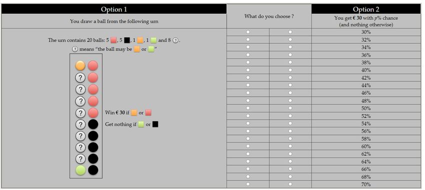
2.2. PE tasks
The second type of tasks our subjects were asked to complete were PE tasks. The best and
worst outcomes were 30 and 0 euros. We measured PEs for bets on the color of a ball drawn
from an Ellsberg urn. The urn contained balls of various colors (red, black, green, yellow, and
blue), but the proportions of yellow and green balls were unknown. Subjects were asked to make
a series of decisions between a given act and lotteries yielding 30 euros with probability p (see
6 In Table 2, we can see that CARA predicts ce( ) = ce( ) + 10 and ce( ) = ce( ) + 20. Obviously, it also predicts
2 1 3 1
ce(3 ) = ce(2 ) + 10, but we do not mention this test in the Table because it would be redundant. Throughout the paper,
redundant tests are omitted.316 A. Baillon, L. Placido / Journal of Economic Theory 181 (2019) 309–332
Table 2
Lotteries and tests.
Lottery Risk CARA [ce(i ) =] [ce(i ) =]
neutral [ce(i ) =] DARA [≥] DRRA [≤]
averse [≤] IARA [≤] IRRA [≥]
seeking [≥]
1 101/2 0 5 1 ce( )
3 4
2 201/2 10 15 ce(1 ) + 10
3 301/2 20 25 ce(1 ) + 20
4 301/2 0 15
5 151/2 10 12.5 1 ce( )
2 3
6 101/4 0 2.5 1 ce( )
3 8
7 201/4 10 12.5 ce(6 ) + 10
8 301/4 0 7.5
9 103/4 0 7.5
10 303/4 20 27.5 ce(9 ) + 20
11 153/4 10 13.75 1 ce( )
2 10
Fig. 2.2. PE-task.
Fig. 2.2 for a screenshot). We define the PE as the midpoint between the lowest p preferred to
the act and the highest p to which the act was preferred.
Table 3 describes the twelve acts and urns that we used to conduct the different tests for
ambiguity neutrality, CAAA and CRAA. For instance, act f1 wins 30 euros if a yellow ball is
drawn from an urn containing 20 balls, 5 being red, 5 being black, and the other 10 being yellow
or green (with at least one of each color).7 Ambiguity arose from the unknown proportions of
yellow and green balls in the urns. We specified that the proportions of yellow and green balls
7 The presence of at least one green and one yellow ball in the urn ensured that acts yielding = 30 0 and = 30 0
1 0
never occurred. This prevented certainty and impossibility effects from distorting our CAAA and CRAA tests. See
subsection 2.3.A. Baillon, L. Placido / Journal of Economic Theory 181 (2019) 309–332 317
Table 3
Acts and tests for ambiguity.
Act Winning color Known Unknown Tests
win 30 euros, # of balls R B L Y (≥ 1) Ambiguity CAAA [pe(fi ) =] CRAA [pe(fi ) =]
0 otherwise or neutral [pe(fi )=] DAAA [≥] DRAA [≤]
G (≥ 1) averse [≤] IAAA[≤] IRAA[≥]
seeking [≥]
f1 Y 20 5 5 – 10 1 pe(f )
2 6
f2 Y &R 20 5 5 – 10 pe(f1 ) + 14
f3 Y &R&B 20 5 5 – 10 pe(f1 ) + 12
f4 Y &R&B 60 5 5 40 10 1 pe(f ); 1 pe(f )
3 3 2 5
f5 Y &R&B 30 5 5 10 10
f6 Y 10 – – – 10
f7 G 20 5 5 – 10 1 − pe(f3 ) 1 pe(f )
2 12
f8 G&R 20 5 5 – 10 1 − pe(f2 ) pe(f7 ) + 14
f9 G&R&B 20 5 5 – 10 1 − pe(f1 ) pe(f7 ) + 12
f10 G&R&B 60 5 5 40 10 1 pe(f ); 1 pe(f )
3 9 2 11
f11 G&R&B 30 5 5 10 10
f12 G 10 – – – 10 1 − pe(f6 )
Y (R, B, L and G) indicates that the color of the ball is “yellow”, “red”, “black, “blue” or “green,” respectively.
were the same for all acts.8 It allows us to model the ambiguous (part of the) urn by the state
space S = {1, ..., 9} representing the number of yellow balls in the urn.9
Act f6 offers 10 s
chances of obtaining 30 euros for a given state s, and act f12 offers 10−s
10
chances of obtaining 30 euros. Hence, the two acts are complementary, which enables us to test
ambiguity aversion (see column 8 in Table 3). Comparing f1 and f2 , observe that f2 adds red to
yellow as a winning color and therefore increases the winning probability for all s by 14 . Under
the CAAA assumption, the PE should also increase by 14 (see column 9 in Table 3 for the other
CAAA tests). Comparing f1 and f6 , observe that the winning color remains the same but that
the urn for act f1 contains 10 more balls than the urn for act f6 . The probability of winning has
been halved in f1 with respect to f6 and thus should be the PE under the CRAA hypothesis (see
the last column of Table 3 for the other CRAA tests).
8 Ellsberg urns create ambiguity because subjects do not know the composition of the urn. We also implemented a
variation of these urns by relating the urn composition to naturally occurring events, namely, whether the Dutch stock
index (AEX) during the experiment would increase or decrease. For these acts, subjects were ambiguity neutral (at the
aggregate level). It could either be that they were not averse towards this particular source of uncertainty (Baillon and
Bleichrodt, 2015 and Baillon et al., 2018 found little to no ambiguity aversion for resembling sources of uncertainty
and similar subjects) or that they did not perceive that this source generated ambiguity. As a consequence, our tests
could not be applied. For the sake of completeness, details on this part of the experiment are reported in supplementary
material.
9 Alternatively, the state space could describe the color of the ball drawn from the urn. Yet, a state space describing
the number of yellow balls, as used here, is simpler to present, remains the same for all acts, and models a uniform
source of ambiguity. We describe the alternative state space(s) in Appendix A and show that our tests remain valid for a
general class of uncertainty-averse preferences if the subjects incorporates the objective information in their perception
of uncertainty.318 A. Baillon, L. Placido / Journal of Economic Theory 181 (2019) 309–332 2.3. Robustness to non-expected utility under risk The theoretical section of this paper is based on the Anscombe-Aumann framework, assum- ing expected utility under risk, but this assumption is usually violated in empirical studies. For instance, Allais (1953) famously showed that people tend to be too attracted by certainty (or impossibility). In the experiment, we avoided certainty and impossibility effects by excluding degenerate lotteries from the acts. This does not solve everything though and we need to assess the robustness of our experiment to non-expected utility. Many non-expected utility models exist but we will focus here on the most used one, Quiggin’s (1981) rank dependent utility (equiva- lently, Tversky and Kahneman’s (1992) prospect theory for gains). In this model, probabilities are weighted, which can bias tests that rely on PEs and shifts of probabilities. We will consider several forms of probability weighting and study the biases they imply. First, we can identify forms of weighting to which the tests are robust. Denote fi (s) = mpi,s 0 the lottery assigned by act fi to state s. With at least one green ball and one yellow ball in the urn, we ensured pi,s ∈ (0, 1) for all i and s. If subjects have a neo-additive weighting function, defined as a function that is linear on (0, 1), then the CAAA tests are still valid, as shown in Appendix C - Observation 4. The appendix also shows that the CRAA tests are robust to power weighting functions. Second, we can estimate the impact of other form of probability weighting. We focus on the popular weighting function proposed by Prelec (1998), w(p) = exp(−(−ln(p))ρ ), with ρ a cur- vature parameter. Expected utility corresponds to ρ = 1. Eliciting Prelec’s weighting function in many different countries, l’Haridon and Vieider (2019) found values of ρ ranging from 0.5 to 1 (with the exception of Nigerian students, for whom the value was 0.27). We assumed the smooth ambiguity model of Klibanoff et al. (2005) and studied the impact of ρ for values between 0.4 and 1.2. For each test described in Table 3, we computed how much the obtained probability equivalent differed from the predicted one (assuming CAAA or CRAA). For instance, if pe(f2 ) was 1.05 times pe(f1 ) + 14 , we said that it had a 5% bias. All computational details and assump- tions are reported in Appendix C. We assessed two cases: (i) if we had run the experiment with no restrictions on the number of green and yellow balls; (ii) with our restriction that there was at least one ball of each color (Y ≥ 1 & G ≥ 1). We found that the restrictions on Y and G more than halved the biases generated by probability weighting. For our CAAA tests, even extreme probability weighting (ρ = 0.4), rarely observed, would not create a bias of more than 5%. For CRAA, one type of tests is sensitive (comparing f6 and f12 to f1 and f7 ), the second type is fair, with biases of less than 5%, and the last one is very robust to Prelec’s probability weighting. This most robust type of tests compares an act with chance of winning between 11/30 and 19/30 to an act with chance of winning between 11/60 and 19/60. For such values, probability weighting seems to be negligible. To account for the risk of probability weighting to affect our results, we will report results in a conservative manner, requiring a deviation of more than 5% of the PEs to classify subjects as non-CAAA or non-CRAA. To classify subjects as CRAA / IRAA / DRAA, we will focus on the robust tests, excluding the comparisons of f6 and f12 to f1 and f7 . 2.4. Participants and organization To conduct the experiment, 78 participants were recruited at Erasmus University Rotterdam (mean age is 21.5; 60% are male). The ordering of the parts (risk and ambiguity) was counter- balanced between participants, and choice tasks were randomized within each part. We ran 8
A. Baillon, L. Placido / Journal of Economic Theory 181 (2019) 309–332         319

sessions on the same day, with 8 to 12 subjects each. A session began with general instructions,
which were read to all subjects who then entered their cubicles. The CE and PE tasks lasted
approximately 30 minutes. Afterward, subjects were paid as described in the next section.

2.5. Incentives

    We used the random incentive system with the slight modification that the choice that would
be played out was determined before the experiment began. For each session and before the
beginning of the experiment, a subject was asked to draw two envelopes in front of the other
subjects and to sign them. The first envelope was drawn from a pile of envelopes containing all
lotteries and acts of the experiment (as described in Tables 2, 3, and 7). The second envelope
was drawn from a pile of 21 envelopes, each containing a different number from 1 to 21, corre-
sponding to a row in the choice lists depicted in Fig. 2.1 or 2.2. At the end of the experiment, the
signed envelopes were opened and the corresponding choice was played out for real money. The
subjects received a show-up fee of 5 euros and an additional amount of up to 30 euros depend-
ing on their choices. On average, the subjects earned 21.50 euros for approximately one hour of
participation. Lotteries and acts were implemented with physical devices (a pair of 10-sided dice
for the lotteries and an urn for the acts). Subjects were informed that the proportions of yellow
and green balls were the same for all acts. In practice, an urn with only yellow and green balls
was prepared before the experiment, and depending on the act that was supposed to be played
for real, the corresponding number of red, black, and blue balls was added.
    Random incentives provided subjects with a mixture over acts and therefore, provided them
with a way to hedge against ambiguity. Overall, in our experiment, being paid for a choice involv-
ing Y as winning color was as likely as being paid for a choice involving G as winning color.
Ambiguity averse subjects who would perceive the whole experiment as one choice may then
behave as if they were ambiguity neutral (Oechssler and Roomets, 2014; Bade, 2015). Hence,
random incentives may lead to underestimate the prevalence of ambiguity aversion. Baillon et
al. (2014) argued that performing the randomization before the resolution of the uncertainty
(and even before choices are made) can mitigate this problem. We followed this procedure, even
though there is no guarantee that it eliminates hedging concerns.

3. Results

    From our initial sample of 78 subjects, eight who violated dominance in the choice lists
(choosing dominated lotteries or acts) at least three times were removed. In the aggregate analy-
sis, we report the results of two-tailed t-tests. Wilcoxon tests produced similar results.

3.1. Risk

   In a first step, we report the aggregate results of our tests of risk neutrality and constant abso-
lute and relative risk aversion. We measured risk attitude by the difference between the expected
value of the lottery E(i ) and the average certainty equivalent ce(i ). Table 4 shows that, at the
aggregate level, the subjects were risk seeking for lotteries with winning probability 14 and averse
for lotteries with winning probability 34 . For probability 12 , they were risk averse or neutral. This
pattern suggests that our subjects would be better represented by rank-dependent utility than by
expected utility. Appendix D reports the results of maximum likelihood estimation of expected
320 A. Baillon, L. Placido / Journal of Economic Theory 181 (2019) 309–332
Table 4
Tests of risk neutrality, CARA and CRRA.
Test for Risk neutrality [=0] p Result Conclusion
E(1 ) − ce(1 ) 0.46*** (0.14) aversion
E(2 ) − ce(2 ) 0.21 (0.16) neutral
E(3 ) − ce(3 ) 1 −0.1 (0.15) neutral
2
E(4 ) − ce(4 ) 2.71*** (0.52) aversion
E(5 ) − ce(5 ) −0.02 (0.08) neutral
E(6 ) − ce(6 ) −0.49*** (0.15) seeking
E(7 ) − ce(7 ) 1 −0.74*** (0.17) seeking
4
E(8 ) − ce(8 ) −0.90** (0.35) seeking
E(9 ) − ce(9 ) 1.11*** (0.21) aversion
E(10 ) − ce(10 ) 3 1.44*** (0.21) aversion
4
E(11 ) − ce(11 ) 0.93*** (0.10) aversion
Test for CARA [=0]
ce(2 ) − [ce(1 ) + 10] 0.23 (0.16) CARA
ce(3 ) − [ce(1 ) + 20] 0.55*** (0.17) DARA
ce(7 ) − ce(6 ) + 10 0.29 (0.19) CARA
ce(10 ) − ce(9 ) + 20 −0.31 (0.21) CARA
Test for CRRA [=0]
ce(1 ) − 13 ce(4 ) 1.33*** (0.42) IRRA
ce(5 ) − 12 ce(3 ) −0.05 (0.17) CRRA
ce(6 ) − 13 ce(8 ) 0.56 (0.38) CRRA
ce(11 ) − 12 ce(10 ) −0.42 (0.29) CRRA
*** , ** , and * indicate that the test is significant at 1, 5, and 10%, respectively. Not rejecting
the null hypothesis is interpreted as risk neutrality, CARA and CRRA. Standard errors are in
parentheses.
utility and of rank-dependent utility for neoadditive and Prelec probability weighting. Introduc-
ing probability weighting substantially increases the fit of the model and neo-additive weighting
fits the data slightly better than the Prelec weighting function. This result should be interpreted
with caution because the experiment was not designed to compare weighting functions but it is
reassuring for the CAAA tests because they are not affected by neo-additive weighting.
Neither CARA nor CRRA was rejected in three out of four tests. Only one of the CARA
tests is rejected in favor of DARA, and one of the CRRA tests is rejected in favor of IRRA.
For comparison, previous empirical results from the literature are mixed. Levy (1994) reported
experimental evidence in favor of DARA but not IRRA, but Eisenhauer (1997) found evidence
for IARA in an empirical study on life insurance. More comparable to our work, Holt and Laury
(2002) found that their experimental data conformed well to IRRA together with DARA (expo-
power utility function).
In a second step, we classified our subjects according to their risk behavior. For all classifica-
tions, we used a 5% error margin to account for the (im)precision of the choice lists. A subject
was classified as CARA (CRRA) if the conditions described in Table 2 were satisfied within
a 5% error margin on average. As seen in the aggregate results, the subjects were risk seeking
for small probabilities and risk averse for large probabilities. To classify subjects as, overall,A. Baillon, L. Placido / Journal of Economic Theory 181 (2019) 309–332 321
Table 5
Classification of subjects depending on their risk attitude.
IARA CARA DARA Total IRRA CRRA DRRA Total
Risk seeking 2 6 2 10 Risk seeking 6 2 2 10
Risk neutral 5 22 1 28 Risk neutral 5 17 6 28
Risk averse 7 22 3 32 Risk averse 14 11 7 32
Total 14 50 6 70 Total 25 30 15 70
(a) Risk attitude and absolute risk aversion (b) Risk attitude and relative risk aversion
IRRA CRRA DRRA Total IRRA CRRA DRRA Total
IARA 2 6 6 14 IARA 2 1 4 7
CARA 18 23 9 50 CARA 9 10 3 22
DARA 5 1 0 6 DARA 3 0 0 3
Total 25 30 15 70 Total 14 11 7 32
(c) Absolute and relative risk aversion (d) Absolute and relative risk aversion (risk averse
subjects only)
more risk averse or seeking, we only considered lotteries 1 to 5 , which involved a 12 chance
of winning. A subject was considered risk neutral if his CE was, on average, within 5% of the
expected value of the lotteries. Subjects whose CEs were lower (higher) than the expected values
by more/than 5% on average were classified as risk averse (seeking).
The results of the classification are reported in Table 5. A large majority of subjects (71%)
displayed CARA (panel (a)). CARA was satisfied by a majority of risk averse subjects (panel
(d)). In terms of relative risk attitude, CRRA was the most common pattern (43%), followed by
IRRA (36%).
3.2. Ambiguity
Table 6 reports the results of the tests for ambiguity neutrality and for constant absolute and
relative ambiguity aversion. At the aggregate level, all tests yielded results in favor of ambiguity
aversion. CAAA and CRAA were systematically rejected in favor of DAAA and DRAA but the
effect sizes are relatively small and still within the range of possible biases due to non-expected
utility under risk such as Prelec-style probability weighting. It is therefore crucial to explore
individual-level data to identify whether the rejection of CAAA and CRAA arises from a small
bias, possibly due to probability weighting and that all subjects exhibit, or from clear and strong
deviations of CAAA and CRAA for part of the sample.
Fig. 3.1 displays the PEs of complementary acts, whose sum should be 1 under ambiguity
neutrality. Many subjects are close to ambiguity neutrality but we see much more and much
stronger deviations in the direction of ambiguity aversion than in the direction of ambiguity
seeking. The sum of PEs of f6 and f12 is further away from 1 for many subjects than the sum of
other PEs for other complementary acts because f6 and f12 concerned the fully ambiguous urns.
Figs. 3.2 and 3.3 depict the PEs of all subjects. They illustrate the magnitude of the violations
of the CAAA and CRAA conditions at the individual level. In Fig. 3.2.a, the (green) circles
represent pe(f2 ) as a function of pe(f1 ), with the size of the circle representing the number of
subjects with this combination. The dashed line pe(f1 ) + 14 represents the CAAA hypothesis,
and a circle above (below) this line indicates DAAA (IAAA). The surrounding dark gray area
represents a ±5% error margin (which could be due to probability weighting, as illustrated in
Fig. C.1), and the light gray area represents a ±10% error margin. Similarly, the (red) squares322 A. Baillon, L. Placido / Journal of Economic Theory 181 (2019) 309–332
Table 6
Tests of ambiguity neutrality, CAAA and CRAA.
Test for ambiguity neutrality [=1] Result Conclusion
pe(f6 ) + pe(f12 ) 0.96* (0.023) aversion
pe(f1 ) + pe(f9 ) 0.95*** (0.013) aversion
pe(f2 ) + pe(f8 ) 0.97*** (0.012) aversion
pe(f3 ) + pe(f7 ) 0.94*** (0.013) aversion
Test for CAAA [=0]
pe(f2 ) − pe(f1 ) + 14 0.03*** (0.009) DAAA
pe(f3 ) − pe(f1 ) + 12 0.02* (0.012) DAAA
pe(f8 ) − pe(f7 ) + 14 0.03*** (0.009) DAAA
pe(f9 ) − pe(f7 ) + 12 0.04*** (0.012) DAAA
Test for CRAA [=0]
pe(f1 ) − 12 × pe(f6 ) −0.03*** (0.009) DRAA
pe(f4 ) − 13 × pe(f3 ) −0.01** (0.004) DRAA
pe(f4 ) − 12 × pe(f5 ) −0.01*** (0.003) DRAA
pe(f7 ) − 12 × pe(f12 ) −0.03*** (0.009) DRAA
pe(f10 ) − 13 × pe(f9 ) −0.02*** (0.004) DRAA
pe(f10 ) − 12 × pe(f11 ) −0.01*** (0.004) DRAA
*** , ** , and * indicate that the test is significant at 1, 5, and 10%, respectively. Not rejecting the
null hypothesis is interpreted as ambiguity neutrality, CAAA and CRAA. Standard errors are in
parentheses.
Fig. 3.1. Magnitude of ambiguity aversion. Notes: Both axes describe PEs. The line represents ambiguity neutrality and
the light (dark) gray areas a 10% (5%) error margin.
in panel (a) represent pe(f8 ) as a function of pe(f7 ). Panel (a) shows that CAAA is a good
approximation of the behavior of many subjects but that a substantial mass of subjects lays above
the gray area. Assuming CAAA for those subjects would imply an error of more than 10%
when predicting their behavior. The circles and squares in panel (b) represent the two CAAAA. Baillon, L. Placido / Journal of Economic Theory 181 (2019) 309–332 323
Fig. 3.2. Magnitude of violations of the CAAA conditions. Notes: Both axes describe PEs. The line represents CAAA
and the light (dark) gray areas a 10% (5%) error margin (in terms of ordinates). The percentages indicate the proportion
of subject who deviate from CAAA by more than 10% (more than 5% between brackets).
conditions when chances are increased by 1/2. For these PEs, CAAA does not seem to be a
bad approximation for a vast majority of subjects if we are willing to accept errors of up to
10%.
In Fig. 3.3, the dashed lines represent the CRAA conditions. The PEs should be multiplied,
which is represented by a line crossing the origin. Subjects above the CRAA line are DRAA, and
those below are IRAA. The dark (light) gray areas again represent a 5% (10%) error margin. In
all panels, a number of subjects approximately satisfy CRAA but a substantial mass of subjects
is located above the CRAA line, with a deviation of more than 10%. The results in panel (c)
should be taken with caution, because they correspond to the tests that were the least robust to
probability weighting according to our robustness analysis.
Table 7 reports the classification of subjects according to their ambiguity behaviors. We used
classification rules similar to those used for risk attitude and compatible with our robustness
analysis, with an error margin of 5% to reflect the possible impact of probability weighting.
For each subject, we computed the average deviation from the conditions given in Table 3 but
excluded the two CRAA tests that were especially sensitive to probability weighting. Subjects
were almost equally distributed between CAAA and DAAA (panel (a)). DRAA was found for
the majority of ambiguity-averse subjects, and most DAAA subjects were also DRAA. Some
subjects could be classified as ambiguity neutral (if they were slightly ambiguity averse for some
acts and slightly ambiguity seeking for others) and still classified as DAAA if the switch from
averse to seeking was consistent across tests. The DAAA-DRAA patterns was also confirmed for
ambiguity averse subjects (panel (d)).
3.3. Impact of wealth on ambiguity attitudes
Combining our results about risk and ambiguity, we could classify CARA subjects with the
definitions of Cerreia-Vioglio et al. (2017). A total of 50 subjects were identified as CARA. As324 A. Baillon, L. Placido / Journal of Economic Theory 181 (2019) 309–332 Fig. 3.3. Magnitude of violations of the CRAA conditions. Note: Both axes describe PEs. The line represents CRAA and the light (dark) gray areas a 10% (5%) error margin (in terms of ordinates). The percentages indicate the proportion of subject who deviate from CAAA by more than 10% (more than 5% between brackets). explained in Section 1.3, for risk neutral subjects, W-CAAA [W-DAAA,W-IAAA] agrees with CAAA [DAAA,CAAA]. Indeed, for subjects whose utility is linear, if the degree of ambiguity aversion remains constant when utility increases (CAAA) then it also remains constant when wealth increases (W-CAAA). A majority of risk neutral subjects were classified as W-CAAA, followed by W-DAAA (Table 8, panel (a)). For risk averse subjects, the equivalence between CAAA and W-CAAA does not hold any- more. For such subjects, W-CAAA is equivalent with CRAA. We therefore classified them using their relative ambiguity aversion, as described by Table 1. Risk averse CARA subjects exhibited mostly W-IAAA and W-CAAA in equal share. Table 8 reports the complete results.
A. Baillon, L. Placido / Journal of Economic Theory 181 (2019) 309–332                        325

Table 7
Classification of subjects depending on their ambiguity attitude.
                      IAAA       CAAA         DAAA   Total                              IRAA      CRAA        DRAA   Total
Ambiguity seeking      0          1            5      6         Ambiguity seeking        0         0           6      6
Ambiguity neutral      6         18           11     35         Ambiguity neutral        5        17          13     35
Ambiguity averse       4         10           15     29         Ambiguity averse         5         9          15     29
Total                 10         29           31     70         Total                   10        26          34     70
(a) Ambiguity attitude and absolute ambiguity aversion          (b) Ambiguity attitude and relative ambiguity aversion

               IRAA        CRAA          DRAA        Total                   IRAA            CRAA        DRAA        Total
IAAA            5           2             3          10         IAAA         2               1            1           4
CAAA            5          18             6          29         CAAA         3               4            3          10
DAAA            0           6            25          31         DAAA         0               4           11          15
Total          10          26            34          70         Total        5               9           15          29
(c) Absolute and relative ambiguity aversion                   (d) Absolute and relative ambiguity aversion
                                                               (ambiguity-averse subjects only)

Table 8
Classification of CARA subjects in terms of W-CAAA, W-DAAA, and W-IAAA.
                W-IAAA      W-CAAA        W-DAAA      Total                        W-IAAA W-CAAA W-DAAA Total
Risk seeking     1           1             4           6       Ambiguity seeking    2             0            2      4
Risk neutral     3           8            11          22       Ambiguity neutral    4            14            9     27
Risk averse     10           9             3          22       Ambiguity averse     8             4            7     19
Total           14          18            18          50       Total               14            18           18     50
(a) Risk attitude and impact of wealth                         (b) Ambiguity attitude and impact of wealth

    Overall, the impact of wealth on ambiguity generates a rich variety of behavior. Sadly, the
restriction to CARA decreases the sample size by almost a third and many CARA subjects were
also ambiguity neutral. For non-CARA subjects, we only know that the way their ambiguity
attitudes depend on wealth is irregular, and therefore, that their behavior is non-classifiable in
terms of W-CAAA, W-DAAA or W-IAAA. By contrast, studying the impact of changes of utility,
as in the previous subsection, has the advantage of identifying regularities that are useful in
applications about saving and prevention for instance.

4. Conclusion

   We designed simple tests of CAAA and CRAA based on variations of the Ellsberg examples.
At the aggregate level, we found evidence for DAAA and DRAA. The magnitude of the devia-
tions from CAAA suggests that relying on the common CAAA assumption to predict behavior
at higher utility levels would lead to errors of more than 10% for a substantial proportion of sub-
jects. CAAA and DAAA coexisted in almost equal shares in our sample of subjects. Our findings
seem to encourage the use of ambiguity models that are flexible enough to accommodate changes
in ambiguity attitudes at increased utility levels, such as the smooth ambiguity model (but ex-
cluding exponential and power smooth-ambiguity functions) and the new models of Ghirardato
and Siniscalchi (2015) and Xue (2018). Finally, combining our results about ambiguity with
those obtained for risk showed that an increase of wealth can have mixed effects on ambiguity
aversion.
326 A. Baillon, L. Placido / Journal of Economic Theory 181 (2019) 309–332
Appendix A. Alternative specification of the state space
Let S1 = {Y, G} be the state space for acts 6 and 12 and S2 = {Y, G, R, B} be the state
space for acts 1-3 and 7-9. F1 and F2 are the sets of acts, and 1 and 2 the set of all
measures over S1 and S2 , respectively. We assume that agents have uncertainty averse pref-
erences (UAP) as defined by Cerreia-Vioglio et al. (2011). Such preferences encompass many
ambiguity models in the literature satisfying ambiguity aversion (but that need not satisfy
CAAA or CRAA). According to UAP, v 1 (f 1 ) = min
P ∈1 G1 Eu (f 1 ) dP , P for f1 ∈ F1 and
v2 (f2 ) = minδ◦P ∈o2 G2 Eu (f2 ) dδ ◦ P , δ ◦ P for f2 ∈ F2 , where G1 and G2 are quasicon-
vex (reflecting ambiguity aversion) and increasing in their first variable (reflecting monotonicity).
Subjects were informed that, for acts 1-3 and 7-9, 5 red balls and 5 black balls would be added
to the urn. For consistency, we make the following assumptions:
• Subjects took the objective information into account; therefore, if P (R) = 14 or P (B) = 14 ,
then G2 (t, P ) = +∞.
• Subjects understood that adding red and black balls to the urn did not change the ambiguity
about the number of yellow (green) balls in the urn; therefore, for P satisfying P (R) =
P (B) = 14 , G2 (t, P ) = G1 (t, δ ◦P ) where δ ◦P is uniquely defined by δ ◦P (Y ) = 2 ×P (Y ).
Note that we also assume here that G1 and G2 are scaled in the same way.
This consistency assumption implies that v2 (f2 ) = minP ∈1 G1 Eu (f2 ) dδ ◦ P , P . We fix
u(30) = 1 and u(0) = 0.
• If f1 ∈ F1 , f2 ∈ F2 , f2 (Y ) = f1 (Y ), f2 (G) = f1 (G), and f2 (R) = f2 (B) = 300 0, then
v2 (f2 ) = minP ∈1 G1 P (Y )
2 Eu (f1 (Y )) + 2 − 2
1 P (Y )
Eu (f1 (Y )) , P = v1 12 f1 +
1
2 300 0 .
• If g1 ∈ F1 , g2 ∈ F2 , g2 (Y ) = g1 (Y ), g2 (G) = g1 (G), and g2 (R) = g2 (B) = 301 0, then
v2 (g2 ) = minP ∈1 G1 P (Y )
2 Eu (g1 (Y )) + 2 − 2
1 P (Y )
Eu (g1 (Y )) + 12 , P = v1 12 g1 +
1
2 301 0 .
As a consequence, under the assumption of subjects’ understanding and incorporating the objec-
tive information into their decisions, the valuations (and, therefore, the probability equivalents)
obtained for f2 and g2 are the same as those that would have been obtained for 12 f1 + 12 300 0
and 12 g1 + 12 301 0. Hence, we can still use them to test constant relative and absolute ambiguity
aversion. The same exercise could be performed for the state spaces of acts 4, 5, 10, and 11.
Appendix B. Application to the smooth ambiguity model
Under risk, CARA and CRRA correspond to exponential and power utility, respectively.
We show here that the definitions (and tests) that we use in this paper for ambiguity al-
low us to characterize the curvature of the smooth ambiguity function of Klibanoff et al.
(2005). Recall that f (s) = mps 0 for all s. We set u(m) = 1 and u(0) = 0, which implies that
Eu (f (s)) = smooth ambiguity model, the PEs satisfy the condition ϕ (pe(f )) =
ps . Under the
(S) μ(Q)ϕ Q(s)ps dQ, with ϕ the smooth ambiguity function and μ second order be-
s∈S
liefs over (S). This impliesA. Baillon, L. Placido / Journal of Economic Theory 181 (2019) 309–332 327
ϕ pe αf + (1 − α) = μ(Q)ϕ (1 − α) + α Q(s)ps dQ
(S) s∈S
and
ϕ pe(αf + (1 − α) ) = μ(Q)ϕ α Q(s)ps dQ.
(S) s∈S
It follows that we can apply the usual results for CEs under expected utility to our PEs under
the smooth model. CAAA is thus equivalent to ϕ being an exponential function and CRAA to
ϕ being a power function. This also shows that, unlike ambiguity models assuming CAAA, the
smooth model can accommodate a broader range of ambiguity attitudes if ϕ is not exponential.
Klibanoff et al. (2005, definition 6) defined CAAA as invariance of preferences to increases
in utility. Implementing a direct test of their definition would require observing utility first. Our
test does not rely on such additional measurements but still enables us to study the implication
of their definition (ϕ being exponential).
Appendix C. Deviations from expected utility under risk
Mixtures of acts and lotteries such as αf + (1 − α) gives corresponding mixtures of expected
utility values. In our design, we only use acts such that f (s) = mps 0. Hence, with u normal-
ized such that u(m) = 1 and u(0) = 0, we obtain Eu (f (s)) = ps , Eu αf (s) + (1 − α) =
αps + (1 − α), and Eu αf (s) + (1 − α) = αps . It is therefore crucial that Eu is linear in
probabilities to obtain the properties about probability equivalents introduced in the previous
subsections.
Now assume that expected utility under risk is replaced by rank-dependent utility (Quiggin,
1981). According to that model, with the same normalization of u, a lottery f (s) = mps 0 is
evaluated by w(ps ). The function w is the probability weighting function and is increasing with
w(0) = 0 and w(1) = 1. If w is nonlinear, then w (αps + (1 − α)) = αw(ps ) + (1 − α) may not
hold.
However, if w is linear on one interval of the probability domain, then the CAAA test based
on acts yielding probabilities within that interval are still valid. As noted by Cohen (1992) and
Webb and Zank (2011) (see also Chateauneuf et al., 2007), certainty effects can be accounted for
by rank-dependent utility models with w being neo-additive, i.e., w(p) = a−b 2 + (1 − a) ∗ p for
all p ∈ (0, 1). The neo-additive weighting functions generate jumps at 0 and 1, thus modeling
impossibility and certainty effects. However, it is linear on (0, 1) and we can make use of it to
test invariance to utility shifts.
The following observation will apply to models that combine rank-dependent utility for lotter-
ies with an ambiguity model. It can for instance be applied to a sort of “maxmin rank-dependent
utility”, that could be written as
min Q(s)w (ps ) (C.1)
Q∈C
s∈S328 A. Baillon, L. Placido / Journal of Economic Theory 181 (2019) 309–332
when f is of the form f (s) = mps 0 and with C ⊂ (S), the set of priors. Another example
would be Klibanoff et al.’s (2005) smooth ambiguity model, with non-expected utility for lotter-
ies where f is valued:
μ(Q)ϕ Q(s)w (ps ) dQ. (C.2)
(S) s∈S
Observation 4. Consider an ambiguity model that values risky lotteries by rank-dependent utility
with a neo-additive weighting function and that is invariant to utility shifts. Then Eq. (1.3) still
holds for f of the form f (s) = mps 0 with 0 < ps < (1 − α) (i.e. neither αf + (1 − α) nor
αf + (1 − α) assigns a sure outcome to any state.)
Proof. Under neo-additive rank-dependent utility for risk, an act f assigning a lottery mps 0
yields utility w(ps ) = a−b
2 + (1 − a)ps on state s. Act αf + (1 − α) yields utility 2 + (1 −
a−b
a)(αps + (1 − α)) on state s whereas act αf + (1 − α) only yields utility 2 + (1 − a)(αps ) on
a−b
state s. Hence, the utility on each state is higher by (1 − a)(1 − α) for the former act than for the
latter. We obtain a constant increase of utility across the state space. Now consider an ambiguity
model assigning pe(f ) to f . The value w(pe(f )) = a−b 2 + (1 − a) × pe(f ) can be interpreted
as the subjective value of the act, expressed in the unit of the risk model (rank-dependent util-
ity). Invariance to utility shifts means that adding (1 − a)(1 − α) to each state increases the
value of the act by exactly (1 − a)(1 − α). It must therefore imply w(pe(αf + (1 − α) )) =
w(pe(αf + (1 − α) )) + (1 − a)(1 − α). Solving a−b 2 + (1 − a) × pe(αf + (1 − α) )) =
2 + (1 − a) × pe(αf + (1 − α) )) + (1 − a)(1 − α) gives pe(αf + (1 − α) )) = pe(αf +
a−b
(1 − α) )) + (1 − α). 2
Our CRAA tests are also robust to some weighting functions. The next observation establishes
it.
Observation 5. Consider an ambiguity model that values risky lotteries by rank-dependent utility
with w(p) = bp c defined on [0, 1) and that is invariant to utility multiplication. Then Eq. (1.5)
still holds for f of the form f (s) = mps 0 with ps < 1.
Proof. Act f yields utility bpsc on state s whereas act αf + (1 − α) yields utility bα c psc on
state s. Hence, the utility on each state is multiplied by α c for the latter act with respect to
the former. Consider a model that is invariant to utility multiplication such as (C.1), i.e. mul-
tiplying the utility by α c on each state multiplies the value of the act by the same factor. It
must therefore imply α c × w(pe(f ))c = w(pe(αf + (1 − α)))). Solving α c × b(pe(f ))c =
b(pe(αf + (1 − α) ))c gives α × pe(f ) = pe(αf + (1 − α) )). Note that this reasoning holds
as long as all probabilities are strictly less than 1, that is, certainty is never reached on any state
of the world. 2
We do not have formal results for the Prelec weighting function but can compute how much it
biases the tests for given parameter values. Assume that the subjects’ behavior can be represented
by the smooth ambiguity model as in Eq. (C.2). For further tractability, we assume that μ(Q) =A. Baillon, L. Placido / Journal of Economic Theory 181 (2019) 309–332 329
Fig. C.1. Bias as a function of the probability weighting parameter.
1
|S| if there is s such that Q = 1s and μ(Q) = 0 otherwise. We obtain 1
|S| ϕ (w (ps )). With this
s∈S
formula, we can compute the probability equivalent of each act. We did so assuming ϕ linear
(such that it should satisfy both CAAA and CRAA), exponential (such that it should satisfy
CAAA), and power (such that it should satisfy CRAA). For the exponential and power functions,
we chose an arbitrary parameter (0.5) to illustrate the effect of the curvature of ϕ. Finally, for each
test described in Table 3, we computed how much the obtained probability equivalent differed
from the predicted one (assuming CAAA or CRAA). For instance, if pe(f2 ) was 1.05 times
pe(f1 ) + 14 , we said that it had a 5% bias.
Fig. C.1 displays the biases for all probability equivalents we could predict as a function of ρ,
the weighting function parameter. Continuous lines represent biases if we had run the experiment
with no restrictions on the number of green and yellow balls; dashed lines represent biases with
our restriction that there was at least one ball of each color (Y ≥ 1 & G ≥ 1).You can also read