Contextual Aware Joint Probability Model Towards Question Answering System
←
→
Page content transcription
If your browser does not render page correctly, please read the page content below
Contextual Aware Joint Probability Model Towards
                                                        Question Answering System

                                                              Liu Yang                                      Lijing Song
                                                   Department of Computer Science                  Department of Computer Science
                                                         Stanford University                             Stanford University
arXiv:1904.08109v1 [cs.CL] 17 Apr 2019

                                                     liuyeung@stanford.edu                           lisasong@stanford.edu

                                                                                       Abstract
                                                  In this paper, we address the question answering challenge with the SQuAD 2.0
                                                  dataset. We design a model architecture which leverages BERT’s [2] capability of
                                                  context-aware word embeddings and BiDAF’s [8] context interactive exploration
                                                  mechanism. By integrating these two state-of-the-art architectures, our system
                                                  tries to extract the contextual word representation at word and character levels, for
                                                  better comprehension of both question and context and their correlations. We also
                                                  propose our original joint posterior probability predictor module and its associated
                                                  loss functions. Our best model so far obtains F1 score of 75.842% and EM score
                                                  of 72.24% on the test PCE leaderboad.

                                         1    Introduction
                                         With increasing popularity of intelligent mobile devices like smartphones, Google Assistant, and
                                         Alexa, machine question answering is one of the most popular field of deep learning research. SQuAD
                                         2.0 [6] challenges a question answering system in two respects: first, to predict whether a question is
                                         answerable based on a given context; second, to find a span of answer in the context if the question
                                         is predicted as answerable. It augments the 100,000 questions in SQuAD 1.1 [7] with 50,000 more
                                         unanswerable questions written in purpose to look like answerable ones. Because of the existence of
                                         those unanswerable questions which account for 1/3 of the train set and 1/2 of the dev and test sets, we
                                         design an elaborate joint probability predictor layer on top of our BERT-BiDAF architecture to solve
                                         the answerable classification and span prediction problem in a probability inference way.
                                         There are many efforts tackling the question answer systems and some work already achieve human
                                         level performance. However, common practice of these works actually base on several weird
                                         assumptions which we argue that will introduce tough constraints to the model and limit the model’s
                                         representation capability.
                                         In this paper, we explicitly point out these weird assumptions and give a thorough discussion about
                                         their weakness. We propose our solution to model the question answer problem in a brand new joint
                                         probability way. Given a specific (question, context) pair, we try to make the model to learn the
                                         joint posterior distribution of the binary answerable or not variable and the start/end span variables.
                                         We propose a BERT-BiDAF [2][8] hybrid model to capture the question aware context information
                                         at both character and word levels with the expectation to gather strong signals to help our joint
                                         probability model make decisions.

                                         2    Related Work
                                         On SQuAD leaderboards, all the top works apply BERT word embedding layer. As a pre-trained
                                         bidirectional transformer language model released in late 2018, BERT [2] is highly respectable to
                                         produce context-aware word representation. Adding n-gram masking and synthetic self-training
techniques onto the BERT framework, the current state-of-art model has achieved near human F1 and
EM accuracy with ensembling. On top of BERT emdedding layer, we apply bidirectional attention
mechanism, because it co-attends to both paragraphs and questions simultaneously and is used
by all the top-ranking models for SQuAD. Among them, BiDAF [8] is one of the first and most
important models. The central idea behind BiDAF and its variants [5] is the Attention Flow layer,
that generates a question-aware context representation by incorporating both context-to-question and
question-to-context attentions.
Other competitive approaches to question answering include QANet [9] and Attention-over-Attention
(AoA) [1]. QANet speeds up training by excluding RNNs and using only convolution and self-
attention, where convolution models local interactions and self-attention models global interactions.
AoA models the importance distribution of primary attentions by stacking additional attentions on
top of the primary attentions.
3 Approach
In this section, we formally define the terminology "context" as the paragraph in which we want
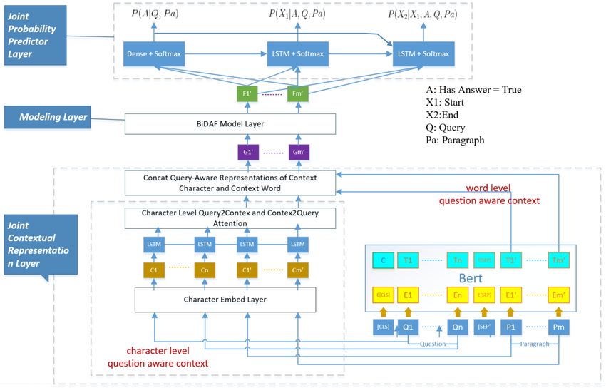
to find the answer while "question" as it literally is. We propose the Joint BERT-BiDAF Question
Answering neural model, Fig.1 illustrates its overall architecture. We keep the "Attention Flow layer"
of BiDAF [8] to produce the question aware context representation at character level. As BERT
[2] can directly provide question aware context at word level, we simply combine the two features
together and feed them into BiDAF’s "Modeling layer" [8] with the expectation to obtain mutually
enhanced context representation (mutual awareness of character/word features, mutual positional
interactions, etc.). Intuitively, the word piece strategy of BERT [2] doesn’t split the normal words,
thus including character embedding can be a good supplement.
In Fig.1, the top layer is our proposed joint probability prediction structure. Unlike the common
practice of inserting a "no-answer" token (e.g baseline and Bert squad) and making the start/end
position of the no-answer case converge to that special token, we try to model the joint distribution of
the binary variable A (has/no answer), the N (context length) value variables X1 (start) and X2 (end)
in a more natural way. We shall give a thorough discussion about this structure in section.3.1.4.
The purpose of introducing the new variable A is to make the model align to the causality that,
given a specific question and context, the existence of a valid span is depend on the
answerable property other than the other way around. It is a big change which result in that we can’t
unify the no-answer loss under the general position entropy loss [2][8], we must design new loss
functions which align to our joint probability structure. Loss function is essential since it exactly
determine every step of the learning update. It is quite trick but interesting to try to figure out a loss
function which value indeed reflect the model’s performance while consistent with the model’s design
philosophy. We shall discuss our loss function exploration in details in section.3.2.
What should be emphasized is that we don’t want to simply reproduce BERT’s success in question
answer problem on SQuAD 2.0 [2]. The main difference between our solution and BERT’s QA
solution 1 is BERT use representations of both question and context to vote for the span prediction
while we only use that of the context. What we really want to do is to verify our original ideas, to
test how well BERT can let the context "aware" the existence of question and to see whether the two
embeddings at different granularity can achieve mutual enhancement.
This section is scheduled in the following way: in section3.1, we discuss about our original model
architecture in general and our effort to implement this architecture. We go through the essential
layers and their back-end techniques but leave the BiDAF[8] details for reference reading. Especially
in section3.1.4, we shall focus on our original joint probability predictor and how we tackle the
answerable problem and the span prediction problem. In section3.2, we shall show several our
original loss functions and their considerations. In section3.3, we introduce the baseline we use and
in section3.4, we briefly summarize the workload of our project. Please keep in mind that we define
our terminology incrementally, once a symbol has been defined, it will be used throughout the rest of
paper.
1
https://github.com/huggingface/pytorch-pretrained-BERT/blob/master/examples/run_
squad.py
23.1 Model Architecture
As illustrated in Fig. 1, we keep the main framework of BiDAF [8] but replace its GloVe [4] word
embedding with BERT contextual word embedding [2] and stack joint probability predictor on top
of it. There are 3 hyper-parameters that determine the computational complexity of our system and
we formally define them to be dlstm , dchar_emb and dbert . dlstm is a uniform hidden dimension for
all LSTM components [3]. dchar_emb and dbert are the dimension of the character word embedding
(output of character level CNN [10]) and the hidden dimension of the BERTBASE [2], respectively.
3.1.1 Embedding Layer
Our embedding layer is built based on BERT base uncased tokenizer.
(i) Word Level Embedding: More precisely, this is token level embedding. Yet BERT doesn’t
split common words thus it is still can be treated as word representation.
(ii) Character Level Embedding: BERT split special words such as name entity into pieces
started with "##", e.g "Giselle" to [’gi’, ’##selle’]. However, each piece is still a character
string from which a dchar_emb dimensional embedding can be generated with character
CNN [10]. Note that "##" in word pieces is ignored.
3.1.2 Joint Contextual Representation Layer
In this layer, we denote the lengths of question and context as Lq and Lc respectively, the character
level representations of question and context are Rcq ∈ RLq ×dchar_emb and Rcc ∈ RLc ×dchar_emb
respectively. We apply the "Attention Flow Layer" of BiDAF[8] to obtain TChar ∈ R8dchar_emb ×Lc
as context representation conditioned on question at character level.
We simply keep the context part from the final encoder layer of BERTBASE to obtain TW ord ∈
Rdbert ×Lc as context representation conditioned on question at word level. We concatenate the two
representations together to produce the joint contextual representation Gctx = [TW ord , TChar ] ∈
R(8dchar_emb +dbert )×Lc .
Figure 1: The Joint BERT-BiDAF Question Answering Model
33.1.3 Modeling Layer
We keep the "BiDAF Modeling Layer"[8] for two reasons.
(i). Although BERT word TW ord can be treat it as positional aware representation but the
character feature TChar can not. We expect TW ord propagates the positional information to
TChar in the mixture process in this layer.
(ii). We want the fine granularity information captured at character level propagates to TW ord .
Actually we expect the two level representations aware the mutual existence and learn how
to cooperate to produce the augmented feature.
The output of the Modeling Layer is F ∈ R(2dlstm +8dchar_emb +dbert )×Lc
3.1.4 Joint Probability Predictor Layer
There are 3 components in our joint probability predictor layer which are responsible to compute
the P (A), P (X1 |A) (start position) and P (X2 |A, X1 ) (end position) respectively. We propose this
structure based on the observation that common practices highly rely on the special "sentry" token
and actually make a solid assumption that P (X1 = 0, X1 = 0|A = 0). We argue that assumption
like this introduces a tough constraint and the effort the model spends on push the (X1 , x2 ) to (0, 0)
will definitely impact the model’s internal mechanism to generate X1 , X2 condition on A = 1.
Our method gives up the special "sentry" token, we choose the natural domain of X1 , X2 to be
{0, 1, · · · , Lc − 1}2 , and relax the P (X1 = 0, X2 = 0|A = 0) constraint to P (X1 = i, X2 =
j|A = 0), ∀i > j, that is, the predicted start position should be larger than the predicted end position
condition on no-answer. The fact P (X1 = i, X2 = j|A = 1), ∀i ≤ j becomes a natural extension of
our concept. Thus we claim that our method does not introduce any inherent contradiction and any
bias assumption.
The connection of the 3 predictors are consistent with the chain rule, the P (X1 |A) predictor relies on
the P (A) predictor, while the P (X2 |A, X1 ) predictor relies on the other two both. Thus the structure
is expected to simulate the joint probability P (A, X1 , X2 ) = P (A)P (X1 |A)P (X2 |A, X1 ).
All the 3 predictors take the output F ∈ R(2dlstm +8dchar_emb +dbert )×Lc of the "Modeling Layer" as
input. For simplicity, we define f = 2dlstm + 8dchar_emb + dbert .
I. P (A) Predictor
In order to compute the binary classification logits, we use a self attention mechanism by setting a
learn-able parameter wA ∈ Rf , the attention vector attA ∈ RLc is computed by Eq.[1]
exp(wT F [:, i])
attA [i] = PLc −1 A , i ∈ {0, 1, · · · , Lc − 1]} (1)
T
k=0 exp(wA F [:, k])
We compute the context summary vector by SA = F attA ∈ Rf . Then we use a learn-able matrix
Wlogit ∈ R2×f to compute the classification logits lA = Wlogits SA ∈ R2 , thus we obtain P (A) as
Eq.[2]
exp(lA [0]) exp(lA [1])
P (A = 0) = , P (A = 1) = (2)
exp(lA [0]) + exp(lA [1]) exp(lA [0]) + exp(lA [1])
In order to propagate the decision of P (A) predictor to P (X1 |A) predictor, we use a learn-able
A
matrix Wprop ∈ R2dlstm ×f to generate a tuple (hA , cA ) = Wprop
A
SA to initialize the LSTM layer of
the P (X1 |A) predictor.
II. P (X1 |A) Predictor
By the bidirectional LSTM layer in P (X1 |A) predictor, we obtain M1 = LST M (F, (hA , cA )) ∈
R2dlstm ×Lc . We use a learn-able vector w1 ∈ R2dlstm to compute the distribution of X1 in Eq.[3]
exp(wT M1 [:, i])
P (X1 = i|A) = PLc −1 1 , i ∈ {0, 1, · · · , Lc − 1}) (3)
T
k=0 exp(w1 M1 [:, k])
4We use the P (X1 |A) ∈ RLc itself as attention to generate the context summary
S1 = M P (X1 |A) ∈ R2dlstm . We concatenate the two context summaries obtained so far
as Sjoint = [SA , S1 ] and propagate the decisions of predictors P (A) and P (X1 |A) to pre-
1
dictor P (X2 |A, X1 ) by initialize its bidirectional LSTM by (h1 , c1 ) = Wprop Sjoint . Here
1 2dlstm ×(f +2dlstm )
Wprop ∈ R is another learn-able matrix parameter in this predictor.
III. P (X2 |A, X1 ) Predictor
By the bidirectional LSTM layer in P (X2 |A, X1 ) predictor, we obtain M2 = LST M (F, (h1 , c1 )) ∈
R2dlstm ×Lc . We use a learn-able vector w2 ∈ R2dlstm to compute the distribution of X2 in Eq.[4]
exp(wT M2 [:, i])
P (X2 = i|A, X1 ) = PLc −1 2 , i ∈ {0, 1, · · · , Lc − 1}) (4)
T
k=0 exp(w2 M2 [:, k])
IV. How to Predict
For a specific instance D[m], from Eq. 2, Eq. 3 and Eq. 4 we have the joint posterior probability as
Eq. 5:
P (A = a, X1 = i, X2 = j|D[m]) = P (A = a|D[m])P (X1 = i|A = a, D[m])P (X2 = j|A = a, X1 = i, D[m])
a ∈ {0, 1}, (i, j) ∈ {0, 1, · · · Lc − 1}2
(5)
We find the maximal negative likelihood p0 = maxi>j {P (A = 0, X1 = i, X2 = j)|D} and the
maximal positive likelihood p1 = maxi≤j {P (A = 1, X1 = i, X2 = j|D)} . If p1 > p0 then we
predict the instance D[m] has answer, otherwise, D[m] has no answer. If D predicted as has answer,
then (start, end) = argmaxi≤j {P (A = 1, X1 = i, X2 = j|D[m])}.
3.2 Loss Function
Assume for a specific instance D[m], the ground truth is (A, X1 , X2 ) = (a, i, j). We propose our
first loss function of our joint probability predictor in Eq. 6. Intuitively, in addition to the normal
binary cross entropy, when an instance D[m] has no answer, we want the probability concentrates on
the maximum likelihood estimation (MLE); when an instance has answer, we just punish the position
loss as common practice.
loss1 (D[m]) = − log(P (A = a|D[m])) + 1(a = 0){−log(maxi>j {P (A = 0, X1 = i, X2 = j|D[m])})}
+ 1(a = 1){−log(P (X1 = i|A = 1, D[m]) − log(X2 = j|A = 1, X1 = i, D[m])}
(6)
For our second loss function, we introduce the distribution U(i, j) as Eq. 7. U(i, j) is a partial
uniform distribution whose probability mass concentrates in the confidence area of P (A = 0|D[m]).
(
2
,i > j
U(i, j) = (Lc −1)Lc (7)
0, i ≤ j
When an instance has no answer, we want the model produces a distribution P (X1 , X2 |D[m]) close
to U. With the Kullback-Leibler divergence, we give our loss2 as Eq. 8:
loss2 (D[m]) = − log(P (A = a|D[m])) + 1(a = 0){KL(U(X1 , X2 )||P (X1 , X2 |D[m]))}
+ 1(a = 1){−log(P (X1 = i|A = 1, D[m]) − log(X2 = j|A = 1, X1 = i, D[m])}
(8)
3.3 Baseline
Our baseline is a modified BiDAF [8] model with word-level embedding provided by cs224n teaching
staff 2 . With the default hyper-parameters, e.g learning rate, decay weight etc. after 30 epochs of
training we get the performance metrics of baseline listed in Table 1.
2
Chapter 4 in DFP Handout and repository cloned from https://github.com/chrischute/squad.git
53.4 Workload
In our project, we install pre-trained BERT from huggingface3 . When reusing the training framework
of the baseline, however, we totally change its tokenization logic in order to integrate BERT. We
write a lot of such foundation code to make the two different system consistent. We write all other
code to implement our proposed BERT-BiDAF hybrid architecture, our joint probability predictor
and loss functions. For ablation purpose, we also implement another answer/no-answer classifier as a
candidate for comparison.
4 Experiments
4.1 Dataset
The dataset we use is Stanford Question Answering Dataset 2.0 (SQuAD 2.0) [6], a reading compre-
hension dataset boosted with additional 50, 000 questions which can not be answered based on the
given context. The publicly available data are split into 129, 941, 6, 078, and 5, 915 examples acting
as the train/dev/test datasets respectively.
Performance is evaluated by two metrics: F1 and EM score. F1 is the harmonic average of precision
and recall. EM (Exact Match) measures whether the system output matches the ground truth answer
exactly, and is stricter than F1. AvNA (Answer vs. No Answer) is an auxiliary metric that measures
how well a model works on labeling a question as has-answer or no-answer.
4.2 Experimental Details
In our experiment, we use BERTBASE [2] which configuration (hidden_size=768, intermediate_-
size=3072, layers=12). For the 3 model complexity identifiers we defined in section3.1, we have
dbert = 768. In order to determine dchar_emb and dlstm and the learning rate, we do grid search
in the range lr ∈ {ke−5 |k ∈ {2, 5, 6, 7, 10}}, dchar_dim ∈ {16, 32, 64, 80}, dlstm ∈ {32, 64, 128}.
We have 60 setting here and for each setting we run 1 epoch on a Nvidia Titan V GPU and sort the
settings by their F1 scores. It takes us about 4 days to get a sorting list and we then fine tune the
model with 3 epochs by trying the high scored settings in order. Finally, we obtain our best model
with lr = 5e−5 , dchar_emb = 16, dlstm = 64.
Fig.2 depicts the performance of our model on dev dataset along with the training process going
on [tensorboard visual output in ’Relative’ mode]. The blue curves represent the baseline while the
yellow ones represent our best model. For all the 3 metrics AvNA, EM and F1, our model beats the
baseline by a significant margin. For the rightmost ’NNL’ subplot, we can identify that the baseline
tends to overfit the dataset in early stage of training, however, for our best model, the signals of
overfitting appear much latter.
Figure 2: Model Performance on dev-set During Training
We also conduct two experiments for ablation. In the first one, we set dchar_emb = 2, that actually
makes the effect of character level embedding negligible. Then the experiment shows both F1 and EM
scores punished by 2+ decrements. In the second one, because BERT[2] claims that its hidden state of
the final layer corresponding to ’[CLS]’ token can be used as the aggregated sequence representation
for classification task, we simply use it for binary answerable classification. In this case, experiment
3
https://github.com/huggingface/pytorch-pretrained-BERT
6shows AvNA decreases by 1.5 while EM and F1 both drop around 2, which indicates the advance of
our output layer.
4.3 Results
We submitted our best model so far to the test PCE leaderboard and obtained the results F1: 75.84,
EM: 72.24. However, in this section, in order to compare with other local implementation, we report
the performance data on dev set in Table 1. We list the performance data of the baseline, our best
model, and the two ablation experiments. The performance differences have been described in the
last section.
Although the overall performance differences are consistent to our arguments that character level
embedding can help and that the joint probability predictor has decent performance, we believe the
performance of our joint probability model can be improved by overcoming 2 difficulties. First, the
overfitting problem. We note that the overfitting problem is significant in our system in the last epoch.
Our best guess towards this problem is the unbalance parameter updating. As BERT uses a strategy
which pushes learning rate to 0 when approaching to the end of training. Thus the gradient may
vanish for BERT module but our upper stacked layers still keep learning, because they are closer to
the gradient source (loss function). This unbalance learning makes the BERT module and the upper
layer out of sync and the discrepancy within our system become bigger and bigger. Second, due to
the limitation of the hardware, we can’t run the size of batch as large as Google. Thus our parameter
updating suffers from the variance problem which makes our system unstable.
Table 1: Model Performance on Dev Set
Metrics
Model F1 EM AvNA
Baseline 59.94 56.55 66.90
Our Best Model 75.48 71.96 79.68
Without CharEmb 73.25 69.87 78.01
[CLS] AvNA Classifier 73.49 69.76 78.23
Human [6] 89.45 86.83 -
5 Qualitative Analysis of Model Errors
5.1 Error Type 1: Wrong Inference
Wrong inference happens when the question and context pair is interpreted incorrectly by our model,
and in some cases attention mechanism focuses on the wrong part of the context. This could happen
because of underfitting in embedding or bidirectional attention, or when the sentence that includes
the answer span is interpreted wrongly due to syntactic complication.
I. False positive example of wrong inference
When reading the long list of Harvard’s alumni, our system, same with original BERT, gets wrong on
many of questions similar to the following ones. When the question asks for "actor starred in The Men
in Black" (or "directer of Noah in 2014"), the system answers "Tatyana Ali" (or "Darren Aronofsky")
simply because s/he is an "actor" (or "film director") according to the context, although "The Men in
Black" or "Noah" is not even mentioned in the paragraph. Because of lack of well-trained embeddings
of entities like film titles, the attention flow layer only focuses on key words such as "actor" and
"director", and generates false positive results distracted by disturbance terms like "The Men in
Black" or "Noah".
Question: What actor starred in the Movie Saving Private Ryan? What actor starred in The Men in
Black? (two questions)
Context: ... comedian, television show host and writer Conan O’Brien; actors Tatyana Ali, Nestor
Carbonell, Matt Damon, ... (1. Harvard University in Appx. A)
Ground Truth: ; (respectively)
Prediction: Tatyana Ali; Tatyana Ali (respectively)
7II. False negative example of wrong inference
In the context, there is no appearance of the key word "status", but the question is looking for such
an answer. Our model fails to draw the correlation between the phrase and the word "status". This
implies insufficiency either in the word embedding of "status" or in the bidirectional attention.
Question: What status has the Brotherhood obtained in the Islamic world?
Context: Despite periodic repression, the Brotherhood has become one of the most influential
movements in the Islamic world ... (2. Islamism in Appx. A)
Ground Truth: one of the most influential movements
Prediction: N/A
5.2 Error Type 2: Imprecise Answer Boundaries
The model points to the right context part but results in imprecise answer span. More sophisticated
techniques to predict start/end positions will help.
I. Example of imprecise answer boundaries
The prediction gives an unnecessary word "that".
Question: What was Shrewsbury’s conclusion?
Context: ... Shrewsbury in 1970, who noted that the reported rates of mortality in rural areas during the
14th-century pandemic were inconsistent with the modern bubonic plague, leading him to conclude
that contemporary accounts were exaggerations... (3. Black Death in Appx. A)
Ground Truth: contemporary accounts were exaggerations
Prediction: that contemporary accounts were exaggerations
5.3 Error Type 3: Confusing Context
Meanwhile, our system also makes mistakes that are prone to human readers. Sometimes we don’t
even agree with the ground truth answers. This error happens because of ambiguous context and
tricky questions.
I. Example of confusing context with imprecise answer boundaries
We and our model don’t agree with the 3 ground truth answers and suspect it makes a coordination
attachment error. The context is confusing with four and’s in a single sentence.
Question: What gained ground when Arab nationalism suffered?
Context: ... Arab nationalism suffered, and different democratic and anti-democratic Islamist
movements inspired by Maududi and Sayyid Qutb gained ground. (4. Islamism in Appx. A)
Ground Truth: anti-democratic Islamist movements, anti-democratic Islamist movements inspired by
Maududi and Sayyid Qutb, anti-democratic Islamist movements
Prediction: different democratic and anti-democratic Islamist movements
II. Example of confusing context without any error
Here is another example in which we don’t agree with the ground truth answer, although our prediction
is exactly the same as the ground truth. According to the context (and China’s history), Kusala is
Tugh Temür’s brother, and was thought to be killed by El Temür; Tugh Temür stayed alive after his
brother’s death. Based on this comprehension, the right answer should be "No Answer" because Tugh
Temür was never killed in the paragraph.
Question: Who was thought to have killed Tugh Temur?
Context: ... Tugh Temür abdicated in favour of his brother Kusala, who was backed by Chagatai
Khan Eljigidey, and announced Khanbaliq’s intent to welcome him. However, Kusala suddenly died
only four days after a banquet with Tugh Temür. He was supposedly killed with poison by El Temür,
and Tugh Temür then remounted the throne. ... (5. Yuan Dynasty in Appx. A)
Ground Truth: El Temür (should be "No Answer")
Prediction: El Temür
86 Conclusion
In this paper, we propose our BERT-BiDAF hybrid architecture, thoroughly explain the intuition, and
show the theoretical derivation of our joint probability predictor and its loss functions. Furthermore,
we demonstrate that our ideas can obtain decent performance on a difficult and highly reputable
problem (SQuAD 2.0) and verify our arguments by ablation experiments. We learn much about model
design and how to conduct a effective learning. We identify that the overfitting and high variance
problems are the two main difficulties which prohibit us form further progress. Our next step is to dig
deeply into the difficulties we are facing and may take question representation into consideration.
Acknowledgments
Thanks to all the CS224 teaching staff for guidance and Microsoft Azure for their great generosity.
References
[1] Yiming Cui et al. “Attention-over-attention neural networks for reading comprehension”. In:
arXiv preprint arXiv:1607.04423 (2016).
[2] Jacob Devlin et al. “Bert: Pre-training of deep bidirectional transformers for language under-
standing”. In: arXiv preprint arXiv:1810.04805 (2018).
[3] Sepp Hochreiter and Jürgen Schmidhuber. “LSTM can solve hard long time lag problems”. In:
Advances in neural information processing systems. 1997, pp. 473–479.
[4] Jeffrey Pennington, Richard Socher, and Christopher D. Manning. “GloVe: Global Vectors
for Word Representation”. In: Empirical Methods in Natural Language Processing (EMNLP).
2014, pp. 1532–1543. URL: http://www.aclweb.org/anthology/D14-1162.
[5] Matthew E Peters et al. “Deep contextualized word representations”. In: arXiv preprint
arXiv:1802.05365 (2018).
[6] Pranav Rajpurkar, Robin Jia, and Percy Liang. “Know What You Don’t Know: Unanswerable
Questions for SQuAD”. In: arXiv preprint arXiv:1806.03822 (2018).
[7] Pranav Rajpurkar et al. “Squad: 100,000+ questions for machine comprehension of text”. In:
arXiv preprint arXiv:1606.05250 (2016).
[8] Minjoon Seo et al. “Bidirectional attention flow for machine comprehension”. In: arXiv
preprint arXiv:1611.01603 (2016).
[9] Adams Wei Yu et al. “Qanet: Combining local convolution with global self-attention for
reading comprehension”. In: arXiv preprint arXiv:1804.09541 (2018).
[10] Xiang Zhang, Junbo Zhao, and Yann LeCun. “Character-level convolutional networks for text
classification”. In: (2015), pp. 649–657.
A Appendix: Full Paragraphs in Analysis
1. Harvard University: Other: Civil rights leader W. E. B. Du Bois; philosopher Henry
David Thoreau; authors Ralph Waldo Emerson and William S. Burroughs; educators Werner
Baer, Harlan Hanson; poets Wallace Stevens, T. S. Eliot and E. E. Cummings; conductor
Leonard Bernstein; cellist Yo Yo Ma; pianist and composer Charlie Albright; composer
John Alden Carpenter; comedian, television show host and writer Conan O’Brien; actors
Tatyana Ali, Nestor Carbonell, Matt Damon, Fred Gwynne, Hill Harper, Rashida Jones,
Tommy Lee Jones, Ashley Judd, Jack Lemmon, Natalie Portman, Mira Sorvino, Elisabeth
Shue, and Scottie Thompson; film directors Darren Aronofsky, Terrence Malick, Mira Nair,
and Whit Stillman; architect Philip Johnson; musicians Rivers Cuomo, Tom Morello, and
Gram Parsons; musician, producer and composer Ryan Leslie; serial killer Ted Kaczynski;
programmer and activist Richard Stallman; NFL quarterback Ryan Fitzpatrick; NFL center
Matt Birk; NBA player Jeremy Lin; US Ski Team skier Ryan Max Riley; physician Sachin H.
Jain; physicist J. Robert Oppenheimer; computer pioneer and inventor An Wang; Tibetologist
George de Roerich; and Marshall Admiral Isoroku Yamamoto.
2. Islamism: Despite periodic repression, the Brotherhood has become one of the most
influential movements in the Islamic world, particularly in the Arab world. For many years
9it was described as "semi-legal" and was the only opposition group in Egypt able to field
candidates during elections. In the Egyptian parliamentary election, 2011–2012, the political
parties identified as "Islamist" (the Brotherhood’s Freedom and Justice Party, Salafi Al-Nour
Party and liberal Islamist Al-Wasat Party) won 75% of the total seats. Mohamed Morsi, an
Islamist democrat of Muslim Brotherhood, was the first democratically elected president of
Egypt. He was deposed during the 2013 Egyptian coup d’état.
3. Black Death: The plague theory was first significantly challenged by the work of British
bacteriologist J. F. D. Shrewsbury in 1970, who noted that the reported rates of mortality in
rural areas during the 14th-century pandemic were inconsistent with the modern bubonic
plague, leading him to conclude that contemporary accounts were exaggerations. In 1984
zoologist Graham Twigg produced the first major work to challenge the bubonic plague
theory directly, and his doubts about the identity of the Black Death have been taken up by a
number of authors, including Samuel K. Cohn, Jr. (2002), David Herlihy (1997), and Susan
Scott and Christopher Duncan (2001).
4. Islamism: The quick and decisive defeat of the Arab troops during the Six-Day War by
Israeli troops constituted a pivotal event in the Arab Muslim world. The defeat along with
economic stagnation in the defeated countries, was blamed on the secular Arab nationalism
of the ruling regimes. A steep and steady decline in the popularity and credibility of secular,
socialist and nationalist politics ensued. Ba’athism, Arab socialism, and Arab nationalism
suffered, and different democratic and anti-democratic Islamist movements inspired by
Maududi and Sayyid Qutb gained ground.
5. Yuan Dynasty: When Yesün Temür died in Shangdu in 1328, Tugh Temür was recalled to
Khanbaliq by the Qipchaq commander El Temür. He was installed as the emperor (Emperor
Wenzong) in Khanbaliq, while Yesün Temür’s son Ragibagh succeeded to the throne in
Shangdu with the support of Yesün Temür’s favorite retainer Dawlat Shah. Gaining support
from princes and officers in Northern China and some other parts of the dynasty, Khanbaliq-
based Tugh Temür eventually won the civil war against Ragibagh known as the War of the
Two Capitals. Afterwards, Tugh Temür abdicated in favour of his brother Kusala, who was
backed by Chagatai Khan Eljigidey, and announced Khanbaliq’s intent to welcome him.
However, Kusala suddenly died only four days after a banquet with Tugh Temür. He was
supposedly killed with poison by El Temür, and Tugh Temür then remounted the throne.
Tugh Temür also managed to send delegates to the western Mongol khanates such as Golden
Horde and Ilkhanate to be accepted as the suzerain of Mongol world. However, he was
mainly a puppet of the powerful official El Temür during his latter three-year reign. El
Temür purged pro-Kusala officials and brought power to warlords, whose despotic rule
clearly marked the decline of the dynasty.
10You can also read