SIGNAL MODEL BASED APPROACH TO JOINT JITTER AND NOISE DECOMPOSITION

Page created by Alice Wells
 
CONTINUE READING
SIGNAL MODEL BASED APPROACH TO JOINT JITTER AND NOISE DECOMPOSITION
SIGNAL MODEL BASED
­APPROACH TO JOINT JITTER
 AND NOISE ­DECOMPOSITION

White paper | Version 01.00 | Adrian Ispas, Julian Leyh, Andreas Maier, Bernhard Nitsch

First published at DesignCon 2020
ABSTRACT
           We propose a joint jitter and noise analysis framework for serial PAM transmission based
           on a parametric signal model. Our approach has several benefits over state-of-the-art
           methods. First, we provide additional measurements. Second, we require shorter sig-
           nal lengths for the same accuracy. Finally, our method does not rely on specific symbol
           sequences. In this paper, we show example measurement results as well as comparisons
           with state-of-the-art methods.

AUTHORS BIOGRAPHY
           Adrian Ispas received Dipl.-Ing. and Dr.-Ing. degrees in Electrical Engineering and
           Information Technology from RWTH Aachen University, Aachen, Germany, in 2007 and
           2013, respectively. Since 2013, he has been with ­Rohde & Schwarz GmbH & Co. KG,
           Munich, Germany, where he is now a Senior Development Engineer in the Center of
           Competence for Signal Processing.

           Julian Leyh obtained his M.Sc. degree in the field of Electrical Engineering from TU
           Munich in 2017 specializing in communications engineering. He then began his pro-
           fessional career as a member of the Center of Competence for Signal Processing at
           ­Rohde & Schwarz. His current focus is on time domain high-speed digital signal analysis.

           Andreas Maier received an M.S. degree in Electrical Engineering and Ph.D. degree
           from the Karlsruhe Institute of Technology (KIT), Germany in 2005 and 2011, respec-
           tively. In 2011, he joined ­Rohde & Schwarz, Munich, Germany. His areas of expertise are
           digital signal processing and signal integrity. He is a lecturer at the Baden-Wuerttemberg
           Cooperative State University Stuttgart, Germany.

           Bernhard Nitsch is the director of the Center of Competence of Signal Processing at
           ­Rohde & Schwarz in Munich, Germany. He and his team focus on signal processing algo-
            rithms and systems in the area of signal analysis, spectral analysis, power measurement,
            security scanners and oscilloscopes. Rohde & Schwarz products contain software, FPGA
            or ASIC based signal processing components developed in the Center of Competence.
            He joined ­Rohde & Schwarz in 2000 and holds a PhD degree in Electrical Engineering and
            Information Technology from Darmstadt University of Technology, Germany and an M.S.
            degree in Electrical Engineering from Aachen University of Technology, Germany. He is
            author of one book and seven technical papers and holds more than 25 patents.

ACKNOWLEDGEMENT
           We want to thank Thomas Kuhwald for initiating the development of the joint jitter and
           noise framework, Guido Schulze for motivating us to submit the paper to DesignCon and
           finally Andrew Schaefer, Guido Schulze and Josef Wolf for their valuable feedback on
           the paper.

2
CONTENTS
             1     Introduction....................................................................................................................................................4

             2     Signal model...................................................................................................................................................5

             3 Jitter and noise decomposition.....................................................................................................................6
           3.1 Source and analysis domains..........................................................................................................................6
           3.2 Decomposition tree..........................................................................................................................................7

             4 Joint jitter and noise analysis framework....................................................................................................8
           4.1 Estimation of model parameters......................................................................................................................9
           4.2 Analysis domains...........................................................................................................................................10

             5     Measurements..............................................................................................................................................11
           5.1     Statistical values and histograms..................................................................................................................11
           5.2     Duty cycle distortion and level distortion......................................................................................................11
           5.3     Autocorrelation functions and power spectral densities..............................................................................11
           5.4     Symbol error rate calculation........................................................................................................................11
           5.5     Jitter and noise characterization at a target SER..........................................................................................12

             6 Framework results........................................................................................................................................13
           6.1 Example analysis...........................................................................................................................................13
           6.2 Signal length influence.................................................................................................................................19

             7     Comparison with competing algorithms.....................................................................................................19

             8     Conclusion....................................................................................................................................................22

             9     References....................................................................................................................................................23

                          Rohde & Schwarz White paper | Signal model based a                                   ­ ecomposition 3
                                                                           ­ pproach to joint jitter and noise d
1 INTRODUCTION
          The identification of jitter and noise sources is critical when debugging failure sources in
          the transmission of high-speed serial signals. With ever increasing data rates accompa-
          nied by decreasing jitter budgets and noise margins, managing jitter and noise sources is
          of utmost relevance. Methods for decomposing jitter have matured considerably over the
          past 20 years; however, they are mostly based on time interval error (TIE) measurements
          alone [1, 2]. This TIE-centric view discards a significant portion of the information present
          in the input signal and thus limits the decomposition accuracy.

          The field of jitter separation was conceived in 1999 by M. Li et al. with the introduction
          of the Dual-Dirac method [3]. The Dual-Dirac method was augmented and improved over
          the next two decades. Originally, it was meant to isolate deterministic from random jit-
          ter components based on the probability density of the input signal’s TIEs. It uses the
          fact that deterministic and random jitter are statistically independent and that determin-
          istic jitter is bounded in amplitude, while random jitter is generally unbounded. Three
          years later, M. Li et al. reported that their Dual-Dirac method systematically overestimates
          the deterministic component [4]. Despite this flaw, modelling jitter using the Dual-Dirac
          model has maintained significance in commercial jitter measurement solutions due to its
          simplicity [5].

          Throughout the years, additional techniques were added to the original Dual-Dirac
          method to separate additional jitter sources such as intersymbol interference (ISI), peri-
          odic jitter (PJ) and other bounded uncorrelated (OBU) jitter. For example, PJ components
          can be extracted using the autocorrelation function [6] or the power spectral density
          [7, 8] of the TIEs, while the ISI part of deterministic jitter can be determined by averag-
          ing periodically repeating or otherwise equal signal segments [13]. Yet another method
          for estimating ISI makes use of the property that ISI can be approximately described as
          a superposition of the effect of individual symbol transitions on their respective TIE [12].
          Once the probability density function of one jitter component is known, any second com-
          ponent can be estimated from a mix of the two by means of deconvolution approaches,
          as long as the components are statistically independent of each other [9, 10, 11].

          Collectively, over 40 IEEE publications and more than 50 patents can be found on the
          topic of jitter analysis alone. Despite this, applications in industrial jitter measurements
          commonly use a combination of the previously described methods [14, 15, 16], all based
          solely on TIEs.

          In this paper, we first introduce a parametric signal model for serial pulse-amplitude mod-
          ulated (PAM) transmission that includes jitter and noise contributions. The key to this
          model is a set of step responses, which characterizes the deterministic behavior of the
          transmission system, similar to the impulse response in traditional communication sys-
          tems. Based on the signal model, we propose a joint jitter and noise analysis framework
          that takes into account all information present in the input signal. This framework relies
          on a joint estimation of model parameters, from which we readily obtain the commonly
          known jitter and noise components. Therefore, we provide a single mathematical base
          yielding the well-known jitter/noise analysis results for PAM signals and thus a consistent
          impairment analysis for high-speed serial transmission systems.

4
known jitter/noise analysis results for PAM signals and thus a consistent impairment
                                        analysis for high-speed
                                      Additionally,     we provideserial
                                                                     deeptransmission    systems.
                                                                            system insight   through the introduction of new mea-
                                      surements, such as what-if signal reconstructions based on a subset of the underlying
                                        Additionally, we provide deep system insight through the introduction of new
                                      impairments. These reconstructions enable the visualization of eye diagrams for a selec-
                                        measurements, such as what-if signal reconstructions based on a subset of the underlying
                                      tion   of jitter/noise
                                        impairments.     Thesecomponents,     thereby
                                                                reconstructions  enableallowing   informed
                                                                                        the visualization  ofdecisions  about
                                                                                                             eye diagrams   for the relevance
                                                                                                                                a selection
                                      ofofthe   selected   components.    Similarly,  we  determine   selective  symbol   error
                                            jitter/noise components, thereby allowing informed decisions about the relevance of  rate (SER)
                                                                                                                                        the
                                      and    bit error  rate (BER)  extrapolations   to allow  fast calculation  of (selective)
                                        selected components. Similarly, we determine selective symbol error rate (SER) and bit   peak-to-peak
                                      jitter
                                        errorandratenoise
                                                     (BER) amplitudes   at low
                                                             extrapolations     error rates.
                                                                             allowing  for a fast calculation of (selective) peak-to-peak

       Signal Model-Based Approach to a Joint Jitter &
                                        jitter and noise amplitudes at low error rates.
                                      The proposed framework is inherently able to perform accurate measurements even

                relativelyNoise           Decomposition
                The proposed framework is inherently able to perform accurate measurements even for
                                      using relatively short input signals. This is due to the significant increase in information
                          short input signals. This is due to the significant increase in information extracted
                                      extracted from the signal. Furthermore, our approach has no requirements regarding spe-
                from the signal. Furthermore, our approach has no requirements regarding specific input
                                      cific inputsequences,
                                       symbol      symbol sequences,     such as compliance
                                                             such as predefined  predefined patterns.
                                                                                              compliance
                                                                                                       On patterns.   On random
                                                                                                           the contrary,   the contrary,
                                                                                                                                     or
                                      the  randominput
                                       scrambled     or scrambled   inputencountered
                                                          data typically  data typically encountered
                                                                                     in real-world     in real-world
                                                                                                   scenarios is ideallyscenarios
                                                                                                                         suited to is
                                                                                                                                   theide-
                                      ally suited to the framework.
                                       framework.
                                                                                Abstract
2 SIGNAL MODEL
          2 Signal Model

                                      The    proposed joint jitter I.
                                       Theproposed                 andI NTRODUCTION
                                                                    andnoise
                                                                        noiseanalysis
                                                                               analysis framework
                                                                                      framework      is based
                                                                                                 is based  on aon   a signal
                                                                                                                 signal   modelmodel   for
                                                                                                                                 for serial
                                      serial
                                       PAMPAM  data data         II.This
                                                          transmission.
                                                     transmission.     S IGNAL
                                                                          This
                                                                          model  M
                                                                               modelODEL
                                                                                       assumes
                                                                                 assumes        the total
                                                                                           the total       signal,
                                                                                                      signal,        i.e. received
                                                                                                              i.e., the   the received   signal
                                                                                                                                    signal
                                       containing all
                                      containing    allcomponents,
                                                        components, totobebe

                                                   ∞

       Signal Model-Based        ∆ [k] · h (tApproach                        toy a+ Joint              Jitter &(1)
                                                   
                y(t) =                            − T [k] −  [k], s) +                     (t).                                                              (1)
                                                             s          sr          clk          h                 −∞         v

                              Noise  the vector Decomposition
                                                 k=−∞
                                                                                                               (1)
                                                                                                                                             
                 Here,s denotes      Here,      of the transmitted PAM symbol sequence 
                                           denotes the vector of the transmitted PAM symbol sequence          and                                and

      Signal Model-Based
              h Δ(t Ts[k]
                 Δ[k]
                    −      
                           [k] −
                             sr s
                                  [k],
                                s[k
                                       =   s)Approach
                                       1] 1
                                           clk
                                              the
                                               = hsymbol
                                                –
                 denotes the step response for the symbol
                                                     s
                                                          h T [k] −atto
                                                      (t −difference
                                                          –     the
                                                             vector 
                                                               t T [k]at
                                                                          symbol
                                                                       symbol   a
                                                                           [k], {s[k],
                                                                         time
                              response for the symbol vector at time , clk
                                                                               sr
                                                                              , 
                                                                                      Joint
                                                                                   index
                                                                                   difference
                                                                                      the
                                                                                             (t,
                                                                                            clk  s) Jitter
                                                                                       k∆h.[k]}).
                                                                                              Moreover,
                                                                                                    at
                                                                                             reference
                                                                                                         ℎ , 
                                                                                                       symbol
                                                                                                           h
                                                                                                       clock time
                                                                                                                   & (2)
                                                                                                                  index      .   ssr       denotes
                                                                                                            the reference clock time at symbol
                                                                                                                      clk
                                                                                                                                                    sr the step

                       k Noise y            Decomposition
                 at symbol index , and  the initial signal value. The disturbance sources are split into
                              index , and –∞ the initial            signal value. The disturbance sources are split into horizontal
                 horizontal  (time) and vertical    (signal level) parts:   is the total horizontal source
                              (time) and vertical (signal
                 disturbance and   is
                                                            ϵ [k] NPlevel)
                                                                       (h) −1 parts: h            is the total
                                                                                                                 horizontal source disturbance and
                                                      Abstract
                                               the total vertical source disturbance. Contrary to traditional
                                                           
                              ϵ v(t
        h [k] = h,P [k] + h,OBU  )  is the  total   vertical
                                        [k] + h,R systems,        source
                                                        [k] = we useA          disturbance.
                                                                                    stepsin(2πf     Contrary    to
                                                                                                        Th,l [k]of+  traditional
                                                                                                                      anφimpulse     communication         sys-     (3)
                                communication                                    a h,l    responseh,linstead              h,l ) + response
                                                                                                                                       h,OBU [k]to+model
                                                                                                                                                       h,R  [k]
                              tems,      we   use   a  step
                                the total signal. This is due response    to  instead
                                                                              the   fact  of
                                                                                          thatan animpulse
                                                                                                     impulse   response
                                                                                                                response     to
                                                                                                                              is  model
                                                                                                                                  neither  the
                                                                                                                                           able total
                                                                                                                                                 to     signal.
                                                                                                                                                     ensure
                                                                      l=0
                              This
                                signalis due   to the under
                                          continuity      fact that     an−1
                                                                  non-linear impulse
                                                                                   (in theresponse
                                                                                             signal levelis neither
                                                                                                             domain)   able   to ensure
                                                                                                                          horizontal        signal continuity
                                                                                                                                         disturbances    nor
                              under
                                able tononlinear        (insymbol
                                                                  N
                                                                     
                                                            the signal I.
                                                                    P (v)   I NTRODUCTION
                                                                             level domain)         horizontal    disturbances         nor able   to repro-
                                            reproduce                       Abstract
                                                                       transition
                                                                            Abstract
                                                                                      asymmetries.        The step    response includes       transmitter,
        v (t) = v,P (t) + v,OBU
                              duce
                                channel,(t)  +and
                                        symbol  v,R   (t) = receiver
                                                   transition
                                                     possibly     asymmetries. A
                                                                     II. S IGNAL   v,l sin(2πf
                                                                                effects, TheM
                                                                                            allstep
                                                                                                ODEL    t + φresult
                                                                                                       response
                                                                                                  ofv,lwhich    v,l )includes
                                                                                                                       +inv,OBU     (t) + v,Rchannel
                                                                                                                                   transmitter,
                                                                                                                             a data-dependent      (t).
                                                                                                                                                     signal and     (4)
                              possibly receiver effects, all of which result in a data-dependent signal disturbance,the
                                disturbance,       i.e.,  inter-symboll=0     interference.      Moreover,      the   step  response      depends    on     i.e.
                                symbol vector          in order toMoreover,
                                                                         account for       effects   like symbol      transition     dependencies     in the s in
                              intersymbol     III.∞system.
                                                      J ITTER
                                                interference.
                                                               InI.
                                                                              N OISE D ECOMPOSITION
                                                                      II NTRODUCTION
                                                                    AND
                                                                 I.the   NTRODUCTION
                                                                                       the   step    response     depends        on   the symbol     vector
                                transmission
                              order to account   for effects            following, we assume the step response to depend only on the
                                                                          like symbol transition dependencies in the transmission sys-
  A.    Source and Analysislast   Domains
                                  y(t)     = and the
                                       symbol            ∆slastII.
                                                              [k]
                                                               II.  · hS        − the  M
                                                                           (t transition:
                                                                       SsrIGNAL
                                                                   symbol           Tclk  [k]
                                                                                           ODEL
                                                                                       Mstep    −response
                                                                                                    h [k], s)to+depend
                                                                                                                      y−∞ +         (t).                             (1)
                              tem. In the following,            we assume IGNAL            ODEL                                onlyv on the last symbol
  B.    Decomposition Treeand the lastk=−∞      symbol transition:
                                              ∞
                                              ∞
                                   y(t)
                                    h sr  =
                                         (t − T
                                          = 1 clk
                                          ∞        ∆
                                                  [k]
                                                   ∞  [k]h··[k],
                                                   ∆ss−
                                                      [k]     h      s)−
                                                              hsrsr (t n=T     (t −−Tclk
                                                                            sr[k]
                                                                         Thclk        h [k],  −+
                                                                                          [k] s)    y−∞{s[k],
                                                                                                 h [k], + v (t).
                                                                                                              ∆s [k]}).                                       (2) (1)
                                                                                                                                                                  (1) (2)
                                   y(t)                            (t∂−   clk [k] − h [k], s) + y−∞ + v (t).
                          yR(h) (t) =        k=−∞
                                             k=−∞      ∆s [k] · n hsr (t − Tclk [k], {s[k], ∆s [k]}) · (−h,R [k])n .                                               (5)
                                              n!                     ∂t
                     Information Classification: General
                                         n=1     k=−∞
                                      We thus have up to N               ⋅ (N
                                                                 PAM NP (h)
                                                                          PAM−1    – 1) step responses for a signal of PAM order N            PAM        .
                                                                        
                              h sr (t  −  T clk [k] −   h [k], s)  =   h sr (t −  T     [k] − h [k],ϵ {s[k],
                                                                                                            [k]      ∆ϵsv[k]}).
                                                                                                                          (t )                     fur- (2)
                              h     The
                                   (t  − total
                                          T      horizontal
                                                [k]
            h [k] = h,P [k] sr+ h,OBUclk[k] +   − h,R
                                                      ∞
                                                              and
                                                            [k],
                                                          h [k] =s)vertical
                                                                     =   h sr  source
                                                                              (t −  T  disturbances
                                                                                      clk
                                                                                 Ah,lclk  [k] −
                                                                                       sin(2πfh,l   [k],  {s[k],
                                                                                                          h      and
                                                                                                  h Th,l [k] + φh,l  ∆ s ) + h,OBU [k] +are
                                                                                                                              ,
                                                                                                                         [k]}). respectively,
                                                                                                                                                h,R [k] (2) (3)
                                    ther decomposed as                  ∂
                              ỹR(h) (t) = −                 ∆s [k] · l=0hsr (t − Tclk [k], {s[k], ∆s [k]}) · h,R [k].                                   (6)
                                                                     NP∂t(v) −1
                                                   k=−∞          NP (h)
                                                                 NP    
                                                                        −1
                                                                    (h) −1
                                                                   
            
       h [k]
           [k] =
              v (t) =  
                = h,P [k]
                            (t)
                        [k] +
                        v,P     +    
                            + h,OBU [k]
                                        [k] +
                                      v,OBU   (t)  +  
                                              + h,R [k]
                                                       [k] =
                                                       v,R   (t)
                                                             =
                                                                  =         A    Av,l sin(2πf
                                                                            Ah,l sin(2πf
                                                                                  sin(2πfh,l T
                                                                                                 v,l t + φ
                                                                                               Th,l [k]
                                                                                                      [k] +
                                                                                                          +φ
                                                                                                             v,l )h,l
                                                                                                                   + v,OBU
                                                                                                              φ )) +
                                                                                                                                 (t) + +v,Rh,R
                                                                                                                      + h,OBU [k]
                                                                                                                                             (t).
                                                                                                                                    [k] +  [k]  [k]     (3) (4)
                                                                                                                                                         (3)
        h           h,P            h,OBU              h,R                         h,l             h,l h,l             h,l         h,OBU            h,R
                                                                    l=0 l=0
                                                                    l=0
                                             III.                   N OISE D ECOMPOSITION
                                                              J ITTER
                                                                  NP (v)AND
                                                                  NP
                                                                         −1
                                                                     (v) −1
                                                          
      
      A.  (t) = 
           Source    (t)
                   and   +  
                     (t) Analysis   (t) +  
                                     Domains    (t) =           A      sin(2πfv,l t + φv,l ) + v,OBU (t) + v,R (t).                           (4)
      vv (t) = v,P
                 v,P     + v,OBU
                              v,OBU (t) + v,R
                                            v,R (t) =           Av,l
                                                                   v,l sin(2πfv,l t + φv,l ) + v,OBU (t) + v,R (t).                       (3) (4)
                                                          l=0
      B. Decomposition Tree                               l=0

                                         III. J ITTER AND N
                                         III.  J ITTER   AND      OISE D
                                                               N OISE     D ECOMPOSITION
                                                                            ECOMPOSITION
 A.
 A.   Source
      Source and
               and Analysis
                     Analysis Domains
                                 Domains
                                     ∞         ∞
                                           1 &
                                        Rohde                  ∂ n | Signal model based a­ pproach to joint jitter and noise d­ ecomposition
                                                Schwarz White paper                                                                           5
 B.
 B.   Decomposition    y
      Decomposition Tree Tree
                         R(h) (t) =                 ∆  s [k] ·    n
                                                                    hsr (t − Tclk [k], {s[k], ∆s [k]}) · (−h,R [k])n .                             (5)
                                          n! n=1        k=−∞
                                                               ∂t
The horizontal and vertical periodic components ϵh,P [k] and ϵv,P (t ), respectively,
          are characterized by the amplitudes Ax,l , the frequencies fx,l and the phases ϕx,l for
          l = 0, … , NP(x) – 1 and x = {h,v}, respectively, and Th,l [k] denotes the relevant point in time
          for the horizontal periodic component l at symbol k. The terms ϵh,OBU [k] and ϵv,OBU (t ) des-
          ignate other bounded uncorrelated (OBU) 1) components, and the random components
          ϵh,R [k] and ϵv,R (t ) denote additive noise for the horizontal and vertical case, respectively.
          At this point, we do not impose any statistical properties on the random components.

3 JITTER AND NOISE DECOMPOSITION
          As introduced in section 2, various effects cause disturbances in transmitted data. The
          transmitter and the channel have the most influence on the step responses that deter-
          mine the data-dependent disturbance of the signal (intersymbol interference). Periodic
          and OBU disturbances make up the remaining deterministic and bounded components.
          Finally, there are random and unbounded disturbances such as thermal noise. Apart from
          being deterministic and bounded, very little information is available about OBU com-
          ponents at the receiver end. Therefore, we omit OBU components from now on. Their
          influence will be visible in the extracted random components.

          3.1 Source and analysis domains
          With the exception of data-dependent components, all disturbances are either of hori-
          zontal or vertical origin. The horizontal components constituting ϵh [k] originate at the
          transmitter, whereas the vertical components in ϵv (t ) may also be added in the channel or
          at the receiver end. The data-dependent components have their origin in the combination
          of the data, i.e. the transmitted symbols, and the step responses that overlap to build the
          signal. We thus define the source domain to be either “horizontal”, “vertical” or “data”.

          Analyzing the disturbances in the time domain is referred to as jitter analysis. Timing
          errors with respect to a reference clock signal are determined and analyzed. This is usu-
          ally done by means of the TIE. However, the disturbances can also be analyzed in the
          signal level domain, which is referred to as noise analysis. In this case, signal level errors
          with respect to reference levels are determined and analyzed at symbol sampling times
          given by a reference clock signal. Fig. 1 depicts the definition of the TIE and the level
          error (LE). The choice between jitter analysis and noise analysis is a choice of the analysis
          domain, which we accordingly define to be either “jitter” or “noise”.

          Fig. 1: TIE and LE definition

                                                                                                                            Signal level
                                                                                   LE
                                                                                                                            Reference level

                                                                                                                            Threshold level

                                                    TIE
                                                                                   Sampling time

                                                            Clock time

                                                  Transition point

          1)
               The word “other” in OBU refers to the nonperiodicity of the disturbance and the word “uncorrelated” to the nonexistence of
               any correlation between the disturbance and the symbol sequence.

6
hsr (t − Tclk [k] − h [k], s) =NP
                                                          h(h) −1− Tclk [k] − h [k], {s[k], ∆s [k]}).
                                                            sr (t                                                          (2
         h [k] = h,P 3.2
                       [k] +Decomposition
                              h,OBU [k] +tree
                                           h,R [k] =             Ah,l sin(2πfh,l Th,l [k] + φh,l ) + h,OBU [k] + h,R [k]
                         The decomposition tree of total jitter   l=0 and total noise is depicted in Fig. 2. It is important to
                                                          NP (h) −1
                         remember that, as shown in        Fig.
                                                               NP2,
                                                                  (v)horizontal
                                                                       −1          disturbances also have an influence in the
    h [k] =   h,P [k] +  
                         noise       [k]
                                 domain
                              h,OBU      +  
                                          and     [k] =
                                                vertical
                                              h,R        disturbancesA  h,l  sin(2πf
                                                                            in the jitter Th,lt[k]
                                                                                       h,ldomain.  + φh,lno
                                                                                                   Thus   ) +matter
                                                                                                              h,OBU [k] + ah,R
                                                                                                                    whether    jit-[k]                                 (3
           v (t) = v,P (t) + v,OBU (t) + v,R (t) =                      Av,l sin(2πf     v,l + φv,l ) + v,OBU (t) + v,R (t).
                         ter or a noise analysis is performed,
                                                            l=0
                                                                  l=0
                                                                      all disturbance components need to be accounted
                         for, i.e. for any analysis domain,      all
                                                          NP (v) −1  source
                                                           AND N OISE          domains are relevant. Moreover, it is generally
                         notv,OBU
                               possible        III.
                                         to directly  J
                                            v,R (t) mapITTER
                                                      = properties   Av,linsin(2πf   D ECOMPOSITION
                                                                               a source                                                                                (4
    v (t) = v,P (t) +              (t) +                                             v,ldomain
                                                                                          t + φv,lto
                                                                                                   )+measurements
                                                                                                       v,OBU (t) + in  an(t).
                                                                                                                     v,R  analy-
    A. Source and Analysis
                         sis domain.Domains
                                        Consider, e.g. thel=0 case of the horizontal random source disturbance ϵh,R [k]
                         only. Its effect on the signal level and thus the noise domain can be described by a Taylor
    B. Decomposition           Tree       III. J ITTER AND N OISE D ECOMPOSITION
                         series of ϵh,R [k] around the mean. For the zero-mean case, we obtain
A. Source and Analysis Domains
                               ∞        ∞
B. Decomposition Tree                1                 ∂n
                 yR(h) (t) =                  ∆s [k] · n hsr (t − Tclk [k], {s[k], ∆s [k]}) · (−h,R [k])n . (4)
                               n=1
                                    n! k=−∞             ∂t
                            ∞
                            1      ∞
                                                   ∂n
             yR(h) (t) =                 ∆
                                         ∞s [k] ·      hsr (t − Tclk [k], {s[k], ∆s [k]}) · (−h,R [k])n .
                                                      n ∂
                                                                                                                                                                       (5
                               n!
                   The first-order approximation
                                                   ∂t
                                                   of equation
                        ỹR(h)
                           n=1(t) =   −
                                   k=−∞        ∆s [k]  · hsr (t(4)−isTgiven  by{s[k], ∆s [k]}) · h,R [k].
                                                                       clk [k],
                                        k=−∞
                                                         ∂t
                                     ∞
                                                    ∂
                   ỹR(h) (t) = −         ∆s [k] · hsr (t − Tclk [k], {s[k], ∆s [k]}) · h,R [k].            (5)                                                       (6
                                    k=−∞
                                                    ∂t

                         We recognize that the horizontal random source disturbances are transformed to the
                         noise domain in a nonlinear manner that depends on the step responses and their deriva-
                         tives 2). Moreover, the inverse step of determining the source disturbance based on the
                         noise disturbance is nontrivial.

                         Fig. 2: Jitter and noise decomposition tree
                         a) Jitter analysis

                              Jitter analysis                    Unbounded
                                                                                                                                         Random horizontal
                                                                                                                                         jitter RJ(h)
                                                                                                       Random jitter RJ
                                                                                                                                         Random vertical
                                                                                                                                         jitter RJ(v)

                                  Total jitter TJ                Bounded
                                                                                                                                         Periodic horizontal
                                                                                                                                         jitter PJ(h)
                                                                                                       Periodic jitter PJ
                                                                                                                                         Periodic vertical
                                                                   Deterministic jitter DJ                                               jitter PJ(v)

                                                                                                       Data-dependent
                                                                                                       jitter DDJ

                              Noise analysis                     Unbounded
                                                                                                                                         Random horizontal
                                                                                                                                         noise RN(h)
                                                                                                       Random noise RN
                                                                                                                                         Random vertical
                                                                                                                                         noise RN(v)

                                  Total noise TN                 Bounded
                         2)
                              For jointly stationary ϵh,R [k] and s [k], and Tclk [k] = kTs with the constant symbol period Ts, the first-order
                                                                                                                                         Periodicapproximation
                                                                                                                                                    horizontal   (5)
                              is cyclostationary. Moreover, for PAM signals of order NPAM > 2 and Gaussian distributed ϵh,R [k], ỹR(h)     (t ) isPN(h)
                                                                                                                                         noise     not Gaussian dis-
                              tributed since the symbol difference Δ s [k] can take on values with different amplitudes.
                                                                                                       Periodic noise PN
                                                                                                                        Periodic vertical
                                       Rohde & Schwarz White paper | Signal
                                                          Deterministic       model based a
                                                                        noise DN                                        noise PN(v)
                                                                                          ­ pproach to joint jitter and noise  ­ ecomposition 7
                                                                                                                               d

                                                                                                       Data-dependent
Deterministic jitter DJ                       jitter PJ(v)

                                                                  Data-dependent
           Fig. 2: Jitter and noise decomposition tree            jitter DDJ

           b) Noise analysis

             Noise analysis            Unbounded
                                                                                      Random horizontal
                                                                                      noise RN(h)
                                                                  Random noise RN
                                                                                      Random vertical
                                                                                      noise RN(v)

                 Total noise TN        Bounded
                                                                                      Periodic horizontal
                                                                                      noise PN(h)
                                                                  Periodic noise PN
                                                                                      Periodic vertical
                                        Deterministic noise DN                        noise PN(v)

                                                                  Data-dependent
                                                                  noise DDN

4 JOINT JITTER AND NOISE ANALYSIS FRAMEWORK
           We propose a framework that encompasses a joint jitter and noise analysis and is based
           on the signal model introduced in section 2. Contrary to state-of-the-art methods, which
           transition from a signal to a TIE representation as a first step, our approach is based
           directly on the total signal. It thus does not discard any information present in the (total)
           signal by using a condensed representation like TIEs do. The core of our framework
           operates independently of the analysis domain (jitter or noise) and considers all source
           domains (horizontal, vertical and data). The jitter and noise results are derived from a joint
           set of estimated model parameters.

           Conceptually, the first step of the framework is to recover a clock that makes it possible
           to decode, i.e. recover, the data symbols. Based on the recovered clock signal and the
           decoded symbols, a joint estimation of model parameters is performed. Specifically, a
           coarse, partly spectrum based estimator recovers rough estimates of the frequencies and
           phases of the vertical periodic components as well as their number. These are then used
           for a fine, least-squares estimator that jointly determines the step responses and the peri-
           odic vertical components. The horizontal periodic components are similarly estimated.
           These estimates, along with the recovered symbols and clock, allow synthesis of signals
           with only selected disturbance components, e.g. the data-dependent signal. We then use
           the total and synthesized signals to transition to the analysis domains and calculate jitter
           and noise values, i.e. TIE and LE values, respectively. Fig. 3 shows a block diagram of the
           framework.

8
Fig. 3: Joint jitter and noise analysis framework

                                                                           Clock and data recovery                 Estimation: step responses             Signal synthesis             Jitter analysis
                                                                                                                   and periodic components

                                                                                                               Coarse estimation     Fine estimation
                                                                                                                                                                  SIGDD
                                                                  SIGT                                                  EST_PV_                        SYNTH_DD
                                                                             CLK_REC      DECODE                                      EST_SR_PV                                                    TIEX
                                                                                                                        COARSE
                                                                                                                                                                                          TIE
                                                                                                                                                                  SIGP(v)
                                                                                                                                                       SYNTH_PV

                                                                                                          TIEP(h) + R                                             SIGDD + P(h)
                                                                                                                        EST_PH_
                                                                                                                                        EST_PH         SYNTH_DD
                                                                                                                        COARSE

                                                                                                                                                                                                   LEX
                                                                                                                                                                                           LE

                                                                                                                                                                                       Noise analysis

                                                                  4.1 Estimation of model parameters
                                                                  The fine estimator that performs a joint estimation of the model parameters is at the core
                                                                             IV. J OINT
                                                                  of the framework   and isJ derived         N OISE
                                                                                                      as follows.
                                                                                              ITTER AND               A NALYSIS
                                                                                                                  First, we need toFtreat  the remaining horizon-
                                                                                                                                     RAMEWORK
                                        A. Estimation             tal disturbances ϵ
                                                                  of Model Parametersh, rem[k] as additive noise for the estimator. Their influence in the signal
                                                                  level domain is quantified as in (5) by linearizing (1) with respect to ϵh, rem[k]:

                                                                       ∞
                                       IV.
     IV. J OINT J ITTER AND N OISE A NALYSISJ OINT  J ITTER
                                             F RAMEWORK        AND  N
                                                (t) ≈ ỹh,rem (t) = − OISE A∆
                                                                            ˇNALYSIS     F RAMEWORK ˇ
                                         yh,rem                               s [k] · h(t − Ťclk [k], {š[k], ∆s [k]}) · h,rem [k]                                                                      (6)
             A. Estimation of Model Parameters
Model Parameters                                                      k=−∞

                                  ∞
                                                                 where š [k]Nis  the decoded
                                                                               P (v)−1
                                                                                             symbol, Δ̌ s [k] the corresponding symbol difference,
                                                           IV.
                                         ˇ s [k] · h(t − Ťclk    t,J{š[k],
                                                               h((v)  šOINT
                                                                        [k]=
                                                                           ,∆ˇ Jss [k]})
                                                                                   [k]
                                                                                      ∞
                                                                                   ITTER  
                                                                                       ) the  AND  [k]N OISE
                                                                                              impulse      ˇ A NALYSIS
                                                                                                        response,   and Τ̌ clk F
                                                                                                                   (7)         [k]RAMEWORK
                                                                                                                                   an estimated   clock time.
 rem (t)   ≈ ỹh,rem (t) = −
                                       y
                                         ∆    v,P (t) ≈ ỹP[k],
                                                (t) ≈ ỹh,rem (t) = −(t)                  · A  v,lˇsin(2π fv,l t + φ̌v,l ) + Av,l (∆
                                                                                             h,rem                                    ˇ f,v,l 2πt +
                                                                                       ∆s [k] · h(t − Ťclk [k], {š[k], ∆s [k]}) · h,rem [k]       ∆φ,v,l ) cos(2π fˇv,l t + φ̌v,l )
                                                                                                                                                                        (7)
                A. Estimation
                          k=−∞        ofh,rem
                                            Model Parameters            l=0k=−∞

       NP (v)−1
                           IV. J OINT J ITTERBy         ANDfurther   approximating
                                                                N OISE       A NALYSIS      theFvertical
                                                                                                   RAMEWORK sinusoidal components, we obtain
                                                             ∞
Estimation
 (t) =        ofAv,l
                 Model
                     sin(2πParameters
                            fˇv,l t + φ̌v,l ) + Av,l (∆
                                                     NPf,v,l
                                                        (v)−1 
                                                             2πt +∆             ∞
                                                                             ) cos(2π   fˇv,l t + φ̌v,l )    (8) ˇ
                                      y(t)    ≈  ỹ(t) 
                                                       =            ∆ˇ φ,v,l
                                                                         [k]   · h    (tˇ−s [k]Ť · [k],  {š[k],
         l=0          v,P (t) ≈ ỹPy(v)         = ≈ ỹh,remA
                                             (t)(t)
                                         h,rem                           − fˇv,l t∆
                                                               (t)v,l=sin(2π
                                                                       s           sr
                                                                                          + φ̌clk    h(t
                                                                                                     ) +  −
                                                                                                          A   Ťclk∆
                                                                                                            v,l (∆
                                                                                                                      s [k]})
                                                                                                                   [k],       +∆
                                                                                                                         {š[k], ˇy−∞  + ỹ· P (v) (t)[k]
                                                                                                                                    [k]})
                                                                                                                    f,v,l 2πt + ∆sφ,v,l ) cos(2π
                                                                                                                                                         + v,R (t) + ỹh,rem
                                                                                                                                               h,remfˇv,l t + φ̌v,l )   (7) (t).
                                                                                                                                                                        (8)
                                                                   k=−∞
                                                                                                 v,l                                                                                                      (7)
                                                                                           k=−∞
  ∞
                                                               l=0
                                                                ∞
                                                                                  IV. J OINT J ITTER AND N OISE A NALYSIS F RAMEWORK
           ˇ s [k] · y
           ∆         hh,rem    Ťclk≈
                       sr (t −(t)
                                                   ˇ s=
                                          {š[k],(t)
                                    [k],ỹh,rem   ∆   [k]})      ˇ sỹ[k]
                                                         − + y−∞ ∆
                                                                 +    P (v)·(t)
                                                                             h(t+−
                                                                                 v,RŤ(t)
                                                                                        clk [k], {š[k],
                                                                                            + ỹh,rem      ˇs(9)
                                                                                                      (t). ∆  [k]})· h,rem [k]                                                      (7)
 k=−∞
                                        A. Estimation
                                                 ∞
                                                          oftheModel
                                                        NP (v)−1
                                                          with           frequenciesParameters fv,l = ƒ̌v,l + Δf,v,l andĥthe      sr phases ϕv,l = ϕ̌ v,l + Δϕ,v,l split into coarse and
                                                       k=−∞
                       y(t)   ≈ ỹ(t)
                                   ≈ỹP=               ˇ [k] · hAsr (tparts  − Ťclk      flˇv,l t0,+…φ̌, v,l
                                                                                               = {š[k],     N∆ˇ)x̂s+= 1.v,l ŷThis    =2πt    +A
                                                                                                                                                       +
                                                                                                                                                      ỹP+y                             ˇv,lỹth,rem           (9)
                                                                                                                                                                                                                (8)
                       v,P (t)               (t) = ∆sremaining
                                            (v)                          v,l sin(2π   for[k],                       [k]})
                                                                                                                P(v) – A
                                                                                                                                + (∆yf,v,l
                                                                                                                                  −∞   yields
                                                                                                                                       −∞           the      ∆(t)
                                                                                                                                                           following
                                                                                                                                                           (v)   φ,v,l+) cos(2π
                                                                                                                                                                             v,R (t) f  +
                                                                                                                                                                            approximation          φ̌(t).
                                                                                                                                                                                                + of   the
                                                                                                                                                                                                      v,l ) total
                              NP (v)−1 sr k=−∞+ signal:
                                        ĥ                  l=0                                                       ∞          p̂
                              x̂ 
                                 = ŷ−∞  = A y                                   ≈A                          −           (10)   ˇ [k] · h(t −                                         ˇ s [k]}) · h,rem [k]
v,P (t) ≈ ỹP (v) (t) =                 p̂Av,l  sin(2π
                                                  ∞        fˇv,l tyh,rem
                                                                     + φ̌v,l(t)) +     ỹh,rem
                                                                                          v,l (∆
                                                                                                   (t)
                                                                                                     f,v,l
                                                                                                          =2πt
                                                                                                          ∞
                                                                                                                    +   ∆       ∆
                                                                                                                             φ,v,ls) cos(2π fv,l t clk
                                                                                                                                                         ˇ Ť +[k],   φ̌v,l{š[k],
                                                                                                                                                                             )          ∆
                                                                                                                                                                                      (8)
                                                                                                        
                                                                                                        ĥsr ˇ k=−∞
                       y(t) ≈l=0   ỹ(t) =             ∆ˇ s [k] · hsr (t −ŷŤDD          [k],
                                                                                      clk(t)     = {š[k],
                                                                                                             ∆∆  ˇ s [k] +
                                                                                                                   s [k]})     ·+ĥsry(t−∞   −+Tcdr   ỹP[k],
                                                                                                                                                           (v) (t)
                                                                                                                                                                 ∆ˇ s+     v,R
                                                                                                                                                                        [k])    +(t)    + ỹh,rem (t). (10)
                                                                                                                                                                                     ŷ−∞                       (9)
                                                                                                                                                                                                               (8)
                        ∞                                                                x̂   =       ŷ −∞ = A y
          ŷDD (t) =  ∞       ˇ s [k] · ĥsr (tk=−∞
                               ∆                 − Tcdr [k], ∆ ˇ s [k]) + ŷ−∞NP (v)−1 k=−∞               p̂               (11)
                                                                                                     NP (v) −1
y(t) ≈ ỹ(t) = k=−∞∆          ˇ s [k] · hsr (tv,P− (t)
                                                     Ťclk≈
                                                          [k], ỹP{š[k],
                                                                    (v) (t)  ∆ˇ= s [k]})       +   y
                                                                                                   A−∞
                                                                                                      v,l  +
                                                                                                           sin(2πỹ     fˇ (t)t + φ̌
                                                                                                                     P (v)v,l            v,R
                                                                                                                                            v,l )(t)
                                                                                                                                                   ++    Av,lỹh,rem
                                                                                                                                                                (∆f,v,l (t).2πt +     (9)∆φ,v,l ) cos(2π fˇv,l t + φ̌v
                       NP (v) −1                          The coarse          estimates
                                                                                ŷ        (t)   and
                                                                                                 =     the
                                                                                                         ĥ   above  Â   approximations
                                                                                                                              sin(2π         f ˆ    t  +  can
                                                                                                                                                            φ̂   be). used to perform            a (fine) joint
                     k=−∞                                                         ∞
                                                                                   P (v)
                                                                                       l=0                  sr           v,l                    v,l            v,l
                                                  ˆ       least-squares           estimation         of
                                                                                                     · −∞the    step
                                                                                                                 −       responses            and      the   vertical     periodic      components:
         ŷP (v) (t) =           Âv,l sin(2π fv,l t + φ̂v,l   ). (t) =
                                                             ŷDD                         x̂∆ˇ= s [k] ŷ  ĥsr (t
                                                                                                          l=0         = TA      +
                                                                                                                           (12)[k],         ˇ
                                                                                                                             cdr y ∆s [k]) + ŷ−∞                                                             (10)
                                                                                                                                                                                                             (11)
                         l=0                                         ∞                                  p̂
                                                                        ĥsr
                                                                                k=−∞
                                                                                   ˇ                                                           ˇ s [k]}) + y−∞ + ỹP (v) (t) + v,R (t) + ỹh,rem (
                                                y(t) ≈ ỹ(t)       =ŷ−∞  P  N  ∆  s A y sr −
                                                                                        [k]
                                                                                         −1   +·  h    (t  T            [k],−{š[k],
                                                                                                                 Ťclk[k]          T           ∆                                    (10)
                                                          x̂   =                    =                                                                   (v) [k]                                                (9)
                                                                                     (v)
                          Tsig,T [k] − Tsig,DD+P (v) [k]                                                       sig,T       (13)       sig,DD+P
                                                                       k=−∞        ∞                                 ˆ
                                                           ŷP (v) (t)p̂=                      Â  v,l sin(2π fv,l t + φ̂v,l ).
                                                                                             ˇ s [k] · ĥsr (t − Tcdr [k], ∆                 ˇ s [k]) + ŷ−∞                                                 (12)
 ins                              B. Analysis Domains        ŷDD (t) = l=0 ∆                                                                                                                               (11)
                                                     ∞ with the estimate vector x̂ containing the Nĥ
                                                                                k=−∞
                                                                                                                                        sr srestimates of the step responses in the
                                                             ˇ
                                                          vector      ĥ   ,  the    (v) −1 signalˇvalue estimate
                                                                                NPinitial                               x̂   =       ŷ −∞ , and
                                                                                                                                                 =A           +
                                                                                                                                                           the y estimates (11)     of the frequencies,
                        TIEX [k]  ŷDD
                                     = T(t)sig,X=[k] − Tcdr∆ [k]s [k] ·srĥsr (t   −Tsig,T
                                                                                        Tcdr [k][k],−  ∆T  s [k])     + (14)
                                                                                                                           ŷ−∞      [k]                                                                     (13)
                                                                                                        TIE         [k]
                                                                                                              sig,DD+Pˆ   =      T           [k]    −    T      [k]
                                                                                                                               + φ̂v,lp̂).components in the vector p̂ .
                                                                                                                                (v)
                                                                                                                                                                                                              (12)
                                                    k=−∞phases,
                                                           ŷP (v) (t)and  = amplitudes        Âv,lofsin(2π
                                                                                                         the verticalfv,l t periodic
                                                                                                                X                  sig,X                    cdr

                  B. Analysis DomainsNP (v) −1                                      l=0
                                                      
                         TIET [k]        TIED
                                      = (t)
                                 ŷP (v)        =[k] + TIERÂ   [k] sin(2π fˆ t + φ̂ ).                         ∞         (15)                                                     (12) d­ ecomposition 9
                                                                   v,l Rohde & Schwarzv,l            v,l paper | Signal   ˇ(16)                                           ˇ sjitter
                  TIEDD+P (h) [k] = TIEDD [k]l=0       + TIEP (h) [k]                   ŷ        White
                                                                                                 (t)    = TIE
                                                                                      Tsig,T [k] − Tsig,DD+P
                                                                                           DD                     T  [k] ∆        TIE
                                                                                                                           =s model
                                                                                                                                 [k]   ·D
                                                                                                                                     [k]  ĥbased
                                                                                                                                              [k]
                                                                                                                                              sr (t +a
                                                                                                                                                     ­−   TIE
                                                                                                                                                       pproach
                                                                                                                                                          TcdrR    to[k]
                                                                                                                                                                 [k],  joint
                                                                                                                                                                         ∆     [k])and+noise
                                                                                                                                                                                          ŷ−∞                (13)
                                                                                                                                 (v)
                  TIEDD+P (v) [k] = TIEDD [k] + TIEP (v) [k]                      TIE         [k]
                                                                                          XTIEDD+P  =    T   k=−∞
                                                                                                           sig,X(h)
                                                                                                                     [k]
                                                                                                                     [k]   −
                                                                                                                           (17)
                                                                                                                           =     TTIE
                                                                                                                                   cdr  [k]
                                                                                                                                          DD     [k]    +    TIE     P (h) [k]                               (14)
y(t) ≈
              y(t)   ≈ ỹ(t)
                       ỹ(t) =  =             ∆ss[k]
                                              ∆     [k] ·· hhsrsr(t (t −   − TTclk         [k], {š[k],
                                                                                      clk[k],      {š[k], ∆      ∆ss[k]})
                                                                                                                        [k]}) +      + yy−∞  −∞ +   + ỹỹPP(v)
                                                                                                                                                            (v)(t)
                                                                                                                                                                 (t) ++ v,R
                                                                                                                                                                           v,R(t)
                                                                                                                                                                               (t) +
                                                                                                                                                                                   + ỹỹh,rem (t). (9)
                                                                                                                                                                                         h,rem(t).    (9)
                 ∞        IV. J OINT J ITTER AND N OISE A NALYSIS F RAMEWORK
                                    k=−∞
                                    k=−∞
    ≈ ỹ(t) =of Model
 )stimation            ∆ˇ s [k] · hsr (t − Ťclk [k], {š[k], ∆                    ˇ s [k]}) + y−∞ + ỹP (v) (t) + v,R (t) + ỹh,rem (t).                                           (9)
                            Parameters
                                    IV. J OINT    TheJmatrix  ITTERAAND       + is the                
                                                                                                       A NALYSIS
                                                                                            Npseudoinverse
                                                                                                OISE                
                                                                                                                     of the           F RAMEWORK
                                                                                                                                            observation matrix and the vector y contains
                k=−∞                                                                                       ĥ
                                                                                                            ĥsrsr
   A. Estimation ofIV.   Model J OINTParameters
                                           J ITTERsamples   ANDofNthe       OISE     total A
                                                                                           x̂
                                                                                           x̂
                                                                                               signal.
                                                                                               NALYSIS
                                                                                               ==     
                                                                                                      ŷŷ−∞Based          on these
                                                                                                                    F RAMEWORK
                                                                                                                              A++yy
                                                                                                                                             estimates and the recovered (or input) clock
                                                                                                                                                                                                    (10)
                                                                                                                                                                                                    (10)
                                                                                                             −∞ =         =A
                                                  signal    ∞  Τ   
                                                                   cdr  [k]    ,     
                                                                                   the     data-dependent                    (DD)      and      the periodic vertical (P(v)) signals can be
imation of Model Parameters                       synthesized         ˇ ĥ   as
                                                                              sr                            p̂
                                                                                                             p̂                        ˇ
              yh,rem (t) ≈ ỹh,rem (t) = −                          ∆     s [k]· h(t −+Ťclk [k], {š[k], ∆s [k]}) · h,rem [k]                                                        (7)
                                                           x̂ =       ŷ ∞
                                                                           −∞ = A y                                                                                                (10)
                      yh,rem (t) ≈ ỹh,rem (t)∞= − p̂  k=−∞
                                                                                ∞ ∞∆ ˇ s [k] · h(t − Ťclk [k], {š[k], ∆                         ˇ s [k]}) · h,rem [k]                       (7)
                                                       
                                                    ŷŷDD                                   ˇˇ    [k] ·· ĥĥsrsr(t(t − − TTcdr                ˇ
                                                                                                                                                ˇ                                                   (11)
                                                                                                                                                                                                    (11)
                                                        DD(t)  (t)ˇ k=−∞
                                                                     ==                     ∆∆ [k]                                 ˇ [k],
                                                                                                                                       [k], ∆   ∆ss[k])
                                                                                                                                                     [k]) + + ŷŷ−∞
            yh,rem (t) ≈ N      (t) = −∞
                           ỹh,rem
                              P (v)−1                            ∆s [k] · h(t −ssŤclk [k],                          {š[k], cdr  ∆   s [k]}) · h,rem [k]
                                                                                                                                                                  −∞
                                                                                                                                                                                    (7)
                                                                           k=−∞
                                                                             k=−∞
 v,P (t) ≈ ỹP (v) (t) =
                                                                ˇ t + φ̌v,l ) + Av,l (∆f,v,l 2πt + ∆φ,v,l ) cos(2π fˇv,l t + φ̌v,l )                                                     (8)
                                     NPA       sin(2π       ˇfsv,l
                                                   k=−∞
                             ŷDD (t)    =v,l
                                         (v)−1              ∆    [k] · N    ĥNPsrP
                                                                                    (v)−1
                                                                                     (t
                                                                                    (v)   −1
                                                                                          − Tcdr [k], ∆            ˇ s [k]) + ŷ−∞                                                 (11)
                                                                      = fˇv,l t + φ̌Â                                                           ). ∆φ,v,l ) cos(2π fˇv,l t + φ̌v,l )           (8) (12)
                               l=0
       v,P (t) ≈ ỹP (v)
                       NP(t)(v)−1=               A
                                                 ŷŷPPv,l(v)
                                              k=−∞       (v) sin(2π
                                                              (t)
                                                               (t) =                                   ) sin(2π
                                                                                                Âv,lv,l
                                                                                                    v,l   +    Av,l (∆
                                                                                                          sin(2π        ffˆˆv,l tt +
                                                                                                                            v,lf,v,l+2πt    v,l+
                                                                                                                                        φ̂φ̂v,l ).                                                  (12)
                                                                                                                                                                                                     (10)
                           
P (t) ≈ ỹP (v) (t)=∞              Av,l        fˇv,l t + φ̌v,ll=0
                                        l=0 NP (v) −1
                                            sin(2π                                   ) + Av,l (∆f,v,l 2πt + ∆φ,v,l ) cos(2π fˇv,l t + φ̌v,l )
                                                                                    l=0
                                                                                                                                                                                    (8)
  (t) ≈ ỹ(t) =            ˇ
                           ŷ
                           ∆    [k] (t)
                                     · h  =
                                         sr (t −      Ť       Â
                                                              [k],     sin(2π
                                                                      {š[k],          ∆ˇ fˆ     t
                                                                                              [k]})   +   φ̂
                                                                                                          +     y  ).       +    ỹ         (t)   +         (t)   +  ỹ      (t). (12)  (9)
                                                  Theclkhorizontal periodic
                              P
                              s (v)                               v,l                       sv,l             v,l   −∞
                           l=0
                             ∞                                                                       components                are    estimated v,R
                                                                                                                                    P (v)
                                                                                                                                                         in a two-step  h,rem
                                                                                                                                                                            approach as above. More
                  k=−∞
       y(t) ≈ ỹ(t)
                  ∞
                      =             ∆ˇ s [k] · hprecisely,
                                                 l=0
                                                    sr (t − Ťclk     the  [k],      TT  sig,T [k]
                                                                                        sig,T
                                                                                      {š[k],
                                                                                estimation       [k]
                                                                                                   ∆     −
                                                                                                         −based
                                                                                                      ˇ is    TTsig,DD+P
                                                                                                         s [k]})
                                                                                                                   sig,DD+P
                                                                                                                       +ony−∞    the(v)+
                                                                                                                                    (v)  [k]
                                                                                                                                           [k]ỹ difference
                                                                                                                                        time    P (v) (t) + v,R (t) + ỹh,rem (t).             (9) (13)
                                                                                                                                                                                                    (13)
                                                                        ˇ 
         B.
 ) ≈ ỹ(t)B.=Analysis
              Analysis ˇ Domains
                       ∆  sDomains
                         k=−∞
                            [k] · hsr (t − Ťclk         [k],[k] {š[k],                                                                                                            (9)
                                                    Tsig,T             − Tĥ∆       sr
                                                                                       s [k]}) + y
                                                                                   sig,DD+P           (v) [k]
                                                                                                             −∞ + ỹP (v) (t) + v,R (t) + ỹh,rem (t).                            (13)              (11)
               k=−∞                                           x̂ = ŷ−∞  ĥ                 =A y     +
                                                                                                                                                                                      (10)
alysis Domains                                    where Τ          sig , T [k]  p̂   and Τsig ,
                                                                                                 sr
                                                                                                       DD + P(v) [k]       are the level crossing time of the total and the
                                                                           x̂ TIE=XXŷ[k]
                                                                                TIE           [k]
                                                                                               −∞=    =    T=
                                                                                                            Tsig,XA+[k]
                                                                                                               sig,X      y −
                                                                                                                         [k]     − TTcdr cdr[k]
                                                                                                                                             [k]                                               (10) (14)
                                                                                                                                                                                                    (14)
                                                  DD + P(v) ĥ            signal,
                                                                             sr            respectively.             Thus an estimate                 of the horizontal periodic (P(h)) contribu-
                                                  tion ∞x̂to  =the ŷlevel          = p̂
                                                                           −∞ crossing         A+ ytimes is obtained and the DD + P(h) signal can(10)                                be synthesized.
                                                   
                                               TIE           [k]ˇ   =      T  sig,X       [k]    −     T  cdr  [k]    ˇ                                                            (14)
                                                                                                                                                                                      (11)
                                                                   s [k]p̂· ĥsr (t − Tcdr [k], ∆s [k]) + ŷ−∞
                                ŷDD (t) =               X     ∆∞
                                                  Summarizing,                    TIE
                                                                                   TIEare
                                                                                   we       TT [k]
                                                                                               [k]able =
                                                                                                       =to   TIE
                                                                                                             TIE      D[k][k] +
                                                                                                                 synthesize
                                                                                                                      D          + TIETIE
                                                                                                                                       signals    [k]with a subset of the underlying source(15)
                                                                                                                                               R[k]
                                                                                                                                               R                                                    (15)
                                                k=−∞
                                         ŷDD (t)        =                  ∆ ˇ s [k] · ĥsr (t − Tcdr [k], ∆                      ˇ s [k]) + ŷ−∞                                             (11)
                                               Ndisturbances.
                                                ∞
                                                     P (v) −1TIE TIEDD+P  DD+P(h)
                                                                                 These [k]     what-if
                                                                                          (h) [k] =    = TIE   signal reconstructions
                                                                                                             TIE      DD[k]
                                                                                                                      DD      [k] + + TIE  TIEPP(h)      allow us to provide new measure- (16)
                                                                                                                                                    (h)[k]
                                                                                                                                                        [k]                                         (16)
                                                  mentsˇ k=−∞   with       selectable             disturbances.  ˇ             For    example,        it  is possible to construct        an eye
                            ŷDD   (t)   =      TIE         ∆ [k][k] =  ·   TIE
                                                                            ĥ      (t    −[k] T
                                                                                               ˆ  +     TIE
                                                                                                        [k],     ∆  [k][k])      +    ŷ                                           (15)
                                                                                                                                                                                   (11)
                                                                                                                                                                                      (12)measure- (17)
                                                               NTIE
                                                                 TIE                                   =+TIE TIE                    + TIE  TIE                                                      (17)
                               ŷP (v) (t) = diagram              Âwith       sr
                                                                             sin(2π           f[k]cdr
                                                                                                 v,l t=        φ̂v,lDD).
                                                            T  s                       D       [k]               R   s                   −∞
                                                                      v,l−1
                                                                          DD+P
                                                                           DD+P data(v)     disturbances
                                                                                          (v)                          and[k]
                                                                                                                      DD      [k]   +
                                                                                                                                chosen              (v)[k]
                                                                                                                                                periodic
                                                                                                                                                  P
                                                                                                                                                  P(v)  [k]disturbances only. The
                                              k=−∞ [k]
                                                                  P (v)
                                      TIEDD+P                        =      TIE  TIE
                                                                                   TIE        [k]     +    TIE                [k]                                                  (16)
                                        ŷP (v)   ments
                                              NP(t)
                                                 (v) −1
                                                       l=0
                                                         = carried Â
                                                        (h)                        out DD
                                                                                      v,l in
                                                                                           D    the =
                                                                                               [k]
                                                                                               [k]
                                                                                            sin(2π
                                                                                            D          =   fˆTIE
                                                                                                             TIE
                                                                                                        analysis     P
                                                                                                              v,l t DD+  domains
                                                                                                                       (h)
                                                                                                                      DD    φ̂[k]
                                                                                                                              [k]   + TIE
                                                                                                                                    +
                                                                                                                               v,l ).      TIE
                                                                                                                                            are PPdescribed
                                                                                                                                                    [k].
                                                                                                                                                    [k].          in the following sections.   (12) (18)
                                                                                                                                                                                                    (18)
                                      TIEDD+P          (v)   [k]    =      TIE        DD     [k]     +    TIE       P (v)   [k]                                                   (17)
                           ŷP (v) (t) = 4.2 Analysis         Âv,ll=0
                                                                       sin(2π  domains   fˆv,l t + φ̂v,l ).                                                                        (12)
                                                TIE     T  D  [k] = TIEDD
                                                            sig,T   [k]     −       T         [k] +(v)
                                                                                       sig,DD+P            TIEP [k].
                                                                                                                [k]                                                                   (13)
                                                                                                                                                                                   (18)
                                                  Based on the total and the synthesized signals, we move away from a signal-centric view
                                                l=0
                                                                     Tsig,T          LE
                                                                                      LE−
                                                                                    [k]      X[k]
                                                                                                [k]sig,DD+P
                                                                                                        == VVXX[k]   [k] −   − VVref ref[k][k]                                                 (13) (19)
                                                                                                                                                                                                    (19)
 nalysis Domains                                                                          the T                              [k]
                                                                                            X
                                                  in order to             obtain                 commonly(v)            known          jitter/noise values. Specifically, we determine              TIEs
                                                            defined
                                                            T     [k]as− T                                                                                               (13)
  B. Analysis Domains                                        sig,T       sig,DD+P (v) [k]
                                                            LE  X [k] = VX [k] − Vref [k]                                                                                (19)
alysis Domains                                              TIEX [k] = TLE
                                                                         LE   TT [k]
                                                                           sig,X [k]  − LE
                                                                                  [k] =
                                                                                      = LE     [k] + LE
                                                                                               [k] +
                                                                                        TcdrDD[k]    LERR[k]
                                                                                                         [k]                                                               (14)                  (20)
                                                                                                                                                                                                 (20)
                                                                                                                                                                                                  (12)

                                                              TIEX [k] = Tsig,X [k] − Tcdr [k]                                                (14)
                                                     where
                                                    LE        Τsig,XLE
                                                        T [k] =
                                                                     [k]Dis[k]
                                                                            the+level
                                                                                   LERcrossing
                                                                                        [k]       time of the signal X = {DD, DD + P(h), DD + P(v), D, T }.
                                                                                                                                     (20)
                                                   TIE
                                                     ForXthe
                                                      TIE      remaining
                                                          [k][k]=T      TIE[k]TIEs,
                                                                                 − we
                                                                                    Tcdrimpose
                                                                                         [k]      the following relationships:      (14)
                                                            T       =sig,X    D [k] + TIER [k]                                         (15)
                                                TIEDD+P (h) [k]TIE=T [k]TIE=DDTIE [k]D+[k]TIE
                                                                                            + PTIE
                                                                                                (h) [k]
                                                                                                     R [k]                             (16) (15)
                                                TIEDD+P
                                                     TIETDD+P
                                                    TIE    [k][k]   =   TIE=
                                                                       [k]
                                                                     TIE        TIE
                                                                                  [k]DD   TIE
                                                                                      + [k]   +  TIE[k]P (h) [k]                       (17) (16)
                                                                =(h)       D [k] + TIE    R [k]                                     (15)
                                                           (v)                DD              P (v)

                                              TIE     TIEDD+P
                                                     TIE    D [k]
                                                           [k]      =
                                                                = (v)   TIE=DD
                                                                       [k]
                                                                     TIE        TIE
                                                                               [k][k] +
                                                                                      TIE
                                                                                    +DD   TIE+
                                                                                          [k]    TIEP (v) [k]
                                                                                              P [k].
                                                                                                 [k]                                   (18) (17)
                                                                                                                                    (16)
                                                     DD+P (h)                        DD                    P (h)
                                               TIEDD+P (v) [k]TIED [k]DD
                                                               = TIE      TIE
                                                                       =[k]  +DDTIE [k]P (v) TIEP [k].
                                                                                         + [k]                               (17) (18) (13)
                                                    TIELE      = TIE
                                                        D [k][k]    VDD      +VTIE
                                                                         [k]−analysis,P [k].                                 (18)
                                                                                                                                (19) to refer-
                                                            X for=the
                                                     Similarly,         [k]
                                                                      noise
                                                                      X         ref [k] we determine LEs that are defined with respect
                                                            ence signal levels:
                                                                          LEX [k] = VX [k] − Vref [k]                                                                                  (19)
                                                            LE
                                                             LEXT[k]
                                                                  [k]=
                                                                     =VLE     −+
                                                                        X [k][k] VrefLE
                                                                                      [k] [k]                                                                            (19)
                                                                                                                                                                           (20)                   (14)
                                                                           D            R

                                                           where VLE
                                                                   X [k]
                                                                       T [k]    LED [k]
                                                                             = signal
                                                                         is the          + LE
                                                                                      value                                                  (20)
                                                                                               R [k] at the symbol sampling times for the signal
                                                                                            obtained
                                                           X = {DD, DD + P(h), DD + P(v), D, T } and Vref [k] is the reference value that depends on
                                                          LE T [k] = LED [k] + LER [k]                                               (20)
                                                           the current symbol value.

            10
LEX [k] = VX [k] − Vref [k]                                                          (19)
                           The remaining LEs are decomposed as in the TIE case, i.e. we use

                           LET [k] = LED [k] + LER [k]                                                           (20)              (15)
                                                                   TABLE I
                                                             S YNTHETIC S ETTINGS
                           and thus the remaining LEs can be computed.
           Property                                    Scenario 1                                     Scenario 2

5 MEASUREMENTS
           Data rate                                   5 Gbps                                         5 Gbps
           Sample rate                                 40 GSa/s                                       20 GSa/s
           Number of symbols                           300 k                                          Variable
           Modulation                                  NRZ, reference levels -1 and +1                NRZ, reference levels -1 and +1
           Symbol pattern Various measurements of         interest can be obtained based on theRandom
                                                       Random                                          TIEs and the LEs intro-
           Rate modulationduced in yection 4.2. TheTriangular
                                                         TIE statistics
                                                                   SSC   can
                                                                         with
                                                                      TABLE I  either
                                                                              -5000ppmbe computed
                                                                                         @  33 kHz   for
                                                                                                      Noneall values or for
           Step response asymmetry                     Fall  time > rise
                            specific subsets, e.g. rising or Sfalling    time
                                                                       edges.
                                                                 YNTHETIC
                                                                                                      None
                                                                                Similarly, the LE statistics can be computed
                                                                            S ETTINGS
           Periodic horizontal disturbance h,P        100 mUI pp @ 20 MHz                            200 mUI pp @ 20 MHz
                            for certain symbol values only. The measurements are briefly presented in the following
           Periodic
            Propertyvertical disturbance  v,P         0.1  pp  @ 100
                                                         Scenario 1    MHz                            0.02  pp @220 MHz
                                                                                                        Scenario
           Random           subsections.
                     horizontal disturbance h,R       205 mUI
            Data rate                                      Gbps rms                                   505 mUI
                                                                                                          Gbps rms
           Random
            Sample vertical
                     rate    disturbance v,R (SNR) 3040dB   GSa/s                                    3520dB
                                                                                                           GSa/s
                          5.1 Statistical values and histograms
           Number of symbols                              300 k                                       Variable
           Modulation We calculate common statistical               valueslevels
                                                          NRZ, reference    like the minimum,
                                                                                  -1 and +1    maximum,
                                                                                                      NRZ, peak-to-peak
                                                                                                            reference levelsvalue,
                                                                                                                             -1 and +1
           Symbol patternpower and standard deviation     Random
                                                            V. (SD)
                                                                 M EASUREMENTS                        Random
                                                                      for both the TIEs and the LEs. Furthermore, we use
           Rate modulation                                Triangular SSC with -5000ppm @ 33 kHz None
                          histogram plots to illustrate the shape of their distribution.
  A.   Statistical  Values
           Step response      and Histograms Fall time > rise time
                          asymmetry                                                                   None
           Periodic horizontal disturbance h,P           100 mUI pp @ 20 MHz                         200 mUI pp @ 20 MHz
  B.   Duty-Cycle    and5.2Level
           Periodic vertical     DutyDistortion
                                       cycle
                             disturbance v,Pdistortion and
                                                          0.1 level
                                                               pp @distortion
                                                                     100 MHz                          0.02 pp @ 20 MHz
           Random horizontal
                          In thedisturbance
                                   context of             20 mUI rms
                                                a jitter analysis,
                                             h,R                   the duty cycle distortion (DCD) is50calculated
                                                                                                         mUI rms as
           Random vertical disturbance v,R (SNR) 30 dB                                               35 dB
                           DCD =         max           {E{TIEDD |hsr,k }} −           min         {E{TIEDD |hsr,k }}               (16)    (2
                                      k=0,...,Nsr −1                             k=0,...,Nsr −1
                                                            V. M EASUREMENTS
   A. StatisticalLD[l]
                   Values     E {x} denotes the expectation of the random variable x and hsr,k the occurrence
                       = and
                      where
                           E{LE  Histograms
                                  DD |level = l + 1|} − E{LEDD |level = l}, l = 0, . . . , NPAM − 1.                                       (2
                      of the k-th step response with k = 0, … , Nsr – 1. The DCD value measures the impact of
   B. Duty-Cycle and Level Distortion
  C. Autocorrelationtwo Functions    and the
                           effects. First, Power        Spectral
                                               differences      in the Densities
                                                                         various step responses, e.g. rising and falling step
                      responses in the case of non-return-to-zero (NRZ) signals (NPAM = 2), and second, a mis-
  D. Symbol Error Rate Calculation
                      match in the signal level thresholds used for determining the TIEs.
                       DCD = max {E{TIEDD |hsr,k }} − min {E{TIEDD |hsr,k }}                                                               (
                                  k=0,...,Nsr −1                                 k=0,...,Nsr −1
                      The level distortion (LD)                       
                                                    for the eye opening l
                                 SER(u) =              Phist [lbin ] ·          pR (v − xhist [lbin ]) dv                                  (2
                  LD[l] = E{LEDD |level =                                v∈e(u)
                                                 lbin l + 1|} − E{LEDD |level = l}, l = 0, . . . , NPAM − 1. (17)                           (
  E.C. Jitter and Noise Characterization
        Autocorrelation  Functions and Power    at a Target
                                                         Spectral   SER Densities
                         is used in the context of noise analysis. It characterizes vertical distortion of the eye open-
   D. Symbol       Error ing
                          Rate
                             dueCalculation
                                  to data-dependent disturbances.

                                             TJ@SER = DJ + σ · c(SER)                                                                      (2
                           5.3 Autocorrelation functions and powerδδspectral
                                                                    
                                                                          RJ
                                                                             densities
                                                
                        Further information can be derived from a spectral view of the TIE and LE tracks. For
  F. Framework Results             SER(u) =            Phist [lbin ] ·        pR (v − xhist [lbin ]) dv                                    (
                        TIEs, a spectral view is not straightforward     to compute since symbol transitions do not
  G. Exemplary Analysis occur between every two
                                                 lbin                  v∈e(u)
                                                     symbols. Usually, this is handled by linear interpolation between
   E.Other
      Jitterstatistics:
              and Noise    Characterization
                        given TIEs. We proposeata different
                                                      a Targetapproach
                                                                    SER in order to avoid the introduction of artifacts.
                          First, compute the autocorrelation function of the TIE track by only considering the given
                          TIE values, then compute the power spectral density (PSD) based on the autocorrelation
  H. Signal Length        Influence            TJ@SER
                          function, thereby obtaining      = DJview
                                                      a spectral                                                                           (
                                                                 δδ + without  any interpolation artifacts.
                                                                      σRJ · c(SER)
                              VI. C OMPARISON AGAINST C OMPETING A LGORITHMS
   F. Framework Results5.4 Symbol error rate calculation
                                                    VII. C ONCLUSION
                       SER plots visualize how varying a single parameter affects the number of correctly
   G. Exemplary Analysis
                       decoded symbols by plotting ACKNOWLEDGMENT
                                                       the SER against the parameter in question. For a jitter anal-
      Other statistics:ysis, the SER is plotted against the sampling time offset used to decode the symbols,
                        while for a noise analysis, the parameter is the decision threshold level of the considered
   H. Signal     Length eye. Symbol errors occur, e.g. when signal transitions take place after the corresponding
                         Influence
                        symbol has been sampled or signal levels do not cross the threshold level of the desired
                        symbol,VI.
                                 respectively. The SERAisGAINST
                                     C OMPARISON                   C OMPETING
                                                          equivalent  to the BER forANRZ
                                                                                     LGORITHMS
                                                                                         signals.
                                                            VII. C ONCLUSION
                                  Rohde & Schwarz White paper | Signal model based a                                   ­ ecomposition 11
                                                                                   ­ pproach to joint jitter and noise d
                                                            ACKNOWLEDGMENT
Symbol pattern                               Random                                       Random
                Rate modulation                              Triangular SSC with -5000ppm @ 33 kHz None
                Step response asymmetry                      Fall time > rise time                        None
                                            Normally,
                Periodic horizontal disturbance   h,P to measure
                                                             100 mUIthe  pp SER,
                                                                            @ 20theMHzsystem under test is200
                                                                                                           usedmUItopp
                                                                                                                     transmit a known symbol
                                                                                                                        @ 20 MHz
                Periodic vertical disturbance
                                            sequence
                                               v,P          0.1 pp   @  100  MHz                         0.02  pp @  20 MHz
                                                       and to evaluate the symbol errors in the received signal. Repeating this mea-
                Random horizontal disturbance     h,R for a 20
                                            surement             mUI rms
                                                             number                                       50 mUI
                                                                         of values of the desired parameter        rmsthe SER plots. Such a
                                                                                                               yields
                Random vertical disturbance v,R (SNR) 30 dB                                              35 dB
                                            measurement setupTABLEusually
                                                                       I      interferes with the regular operation of the system under test
                                            and may Stherefore
                                                       YNTHETICbe   S ETTINGS
                                                                       difficult to accomplish or even yield different results. Additionally,
                                          SER measurements take a very long time for low SER values like 10–12.
   Property                                 Scenario 1         V. M EASUREMENTS Scenario 2
   Data rate                                5 Gbps                                           5 Gbps
       A. rate
   Sample   Statistical Values and Histograms
                                        We propose
                                            40 GSa/s a method to calculate SER plots20based       GSa/s on the jitter or noise values, i.e. the
   Number of symbols                    TIEs300
                                             or LEs,
                                                  k      respectively, and their statistics.Variable
                                                                                               To calculate an SER plot, first select a histo-
       B. Duty-Cycle and Level Distortion
   Modulation                               NRZ,
                                        gram   thatreference   levels
                                                      covers all       -1 anddeterministic
                                                                  desired     +1             NRZ, reference
                                                                                           components         levels
                                                                                                           with  bins-1representing
                                                                                                                        and +1      the desired
   Symbol pattern                           Random                                           Random
                                        analysis domain and a set of probability distribution parameters describing the desired
   Rate modulation                          Triangular SSC with -5000ppm @ 33 kHz None
   Step response asymmetry DCD = random           components
                                            Fall time    > rise timein the
                                                        {E{TIE
                                                                            same analysis domain.     For example, when the SER for all
                                                                                         minNone{E{TIEDD |hsr,k }}                            (21)
                                            max                    DD |hsr,k }} −
   Periodic horizontal disturbance h,P signal
                                            100disturbances
                                         k=0,...,N sr −1 pp @ 20plotted
                                                  mUI              MHz against the      sampling
                                                                                    k=0,...,N200    timeppoffset
                                                                                              sr −1mUI     @ 20 is  desired, we select the TIE
                                                                                                                  MHz
   Periodic vertical disturbance v,P       0.1 pp @
                                        histogram         100 MHz
                                                       covering                              0.02 ppand
                                                                  all deterministic components        @ 20theMHz
                                                                                                              TIE distribution covering all ran-
   Random horizontal disturbance h,R dom20components.
                                                 mUI rms        By choosing histograms and   50 mUI    rms
                                                                                                   distributions  that cover only part of the
   Random vertical disturbance v,R (SNR) 30 dB                                              35 dB
                         LD[l] = E{LEDD |levelsignal
                                    measured    =l+    1|} − E{LEwhat-if
                                                     perturbations, DD |level
                                                                          SER=  l}, can
                                                                              plots  l =be0,generated
                                                                                             . . . , NPAM
                                                                                                        that 1. the user(22)
                                                                                                          − allow
                                          to gain insight into how the SER would change if the user were to resolve certain signal
       C. Autocorrelation Functions   and issues.
                                integrity  PowerThe  Spectral
                                                        information Densities
                                                                         stored in the histogram is, for every bin l bin , the prob-
                                        V.   M  EASUREMENTS
                                ability of hitting that bin P hist [l bin] and the position of that bin x hist [l bin]. Assuming a
       D. Symbol Error Rate Calculation
Statistical Values and Histogramsprobability distribution pR of the random components, we get the SER
Duty-Cycle and Level Distortion                                    
                                 SER(u) =           Phist [lbin ] ·          pR (v − xhist [lbin ]) dv                             (23)
                                                                                                                                    (18)
                                                         lbin               v∈e(u)

       E. Jitter DCD       max {E{TIEDDat|hsr,k
                      = Characterization
                 and Noise           where e (u) = {xa
                        k=0,...,Nsr −1
                                                         }} − SER
                                                        Target
                                                     : position
                                                                    min {E{TIEDD |hsr,k }}
                                                                 x generates
                                                                k=0,...,N
                                                                                                                    (21)
                                                                          sr −1 a decoding error for parameter u } holds informa-
                                    tion about the error conditions. Note that while random disturbances are often assumed
                                    to be Gaussian distributed, this may not be the case in certain scenarios due to the non-
             LD[l] =   E{LEDD |levellinear
                                      =l+     1|}TJ@SER
                                           transformation  = DJ
                                                  − E{LEfrom
                                                           DD |level
                                                                 δδ +=
                                                                source    l},
                                                                       σtoRJ  · lc(SER)
                                                                                  = 0,domain
                                                                           analysis    . . . , N(see  − 1. 3.2).
                                                                                                 PAM section     (22)      (24)
Autocorrelation Functions
     F. Framework   Resultsand Power  Spectral
                                5.5 Jitter        Densities
                                           and noise characterization at a target SER
Symbol
     G.Error  Rate Calculation
         Exemplary  Analysis A number of secondary measurements are derived from the SER calculation. One of
                                         these is TJ@SER, the total jitter at a target SER. This value represents the jitter budget
            Other statistics:
                                                             has to anticipate when trying to reach a target SER. It can be iden-
                                         that a system designer
                                            
                       SER(u)           =tified as
                                                P the[lwidth
                                          hist bin       ] · of the SER
                                                              R      p (vvs.−sampling
                                                                               x [l time
                                                                        hist bin        ]) dvoffset plot at the desired SER.
                                                                                                                         (23)
       H. Signal Length Influence lbin                v∈e(u)
                                Another example is the Dual-Dirac value DJδδ from the Dual-Dirac model. The Dual-Dirac
                              VI.model
Jitter and Noise Characterization C OMPARISON
                                  at   a assumes   thatAthe
                                          Target SER     GAINST   C OMPETING
                                                            deterministic jitter canAonly
                                                                                      LGORITHMS
                                                                                          take on two discrete values and that
                                the relationship VII. C ONCLUSION
                                                    ACKNOWLEDGMENT
                                 TJ@SER = DJδδ + σRJ · c(SER)                                                   (24)        (19)

Framework Results                         holds, where the value c (SER) depends solely on the target SER. Sufficiently low SERs
 Exemplary Analysis                       need to be ensured for the above relationship to hold, otherwise the (Gaussian) random
                                          jitter does not dominate the total jitter.
Other statistics:
                                          For noise analysis, we compute the EH@SER value, which gives the eye height that is
 Signal Length Influence                  achieved at a target SER.

                     VI. C OMPARISON AGAINST C OMPETING A LGORITHMS
                                    VII. C ONCLUSION
                                   ACKNOWLEDGMENT

       12
6 FRAMEWORK RESULTS
         In this section, we present measurement results from the joint jitter and noise analy-
         sis framework presented in section 4. To make the vast amount of measurements and
         comparisons more accessible, we present a single scenario in section 6.1 and use a
         majority of the available results to track down a signal integrity issue and understand its
         implications. In section 6.2, we show how the length of the input signal affects the mea-
         surements and thus the framework’s performance. The scenarios used in this subsection
         are summarized in Table 1. We use a second order phase-locked loop (PLL) with a band-
         width factor of 500 and a damping factor of 0.7 for these scenarios.

         Table 1: Settings for synthetic scenarios

                  Property                                          Scenario 1                          Scenario 2
                  Data rate                                         5 Gbps                              5 Gbps
                  Sample rate                                       40 Gsample/s                        20 Gsample/s
                  Number of symbols                                 300k                                variable
                  Modulation                                        NRZ, reference levels: –1 and +1    NRZ, reference levels: –1 and +1
                  Symbol pattern                                    random                              random
                                                                    triangular SSC with –5000 ppm
                  Rate modulation                                                                       none
                                                                    at 33 kHz
                  Step response asymmetry                           fall time > rise time               none
                  Periodic horizontal disturbance ϵh, P             100 mUI pp at 20 MHz                200 mUI pp at 20 MHz
                  Periodic vertical disturbance ϵv, P               0.1 pp at 100 MHz                   0.02 pp at 20 MHz
                  Random horizontal disturbance ϵh, R               20 mUI RMS                          50 mUI RMS

                  Random vertical disturbance ϵv, R
                                                                    30 dB                               35 dB
                  (SNR)

         6.1 Example analysis
         Throughout this section, we use scenario 1 from Table 1, i.e. a synthetic 5 Gbps NRZ data
         signal with random symbols to show the framework’s capabilities.

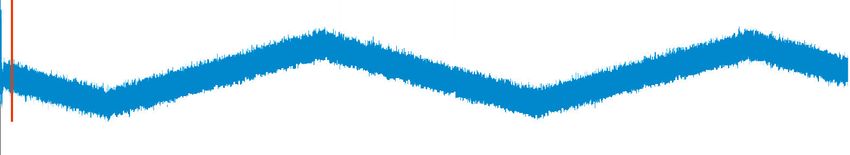
         Fig. 4 shows the data rate over time as recovered by the clock and data recovery (CDR).
         At the very start of the signal, the CDR’s locking behavior can be observed. After the
         lock time (indicated by the red line), the CDR follows a triangular modulation profile of
         –5000 ppm at 33 kHz. Such a modulation profile is commonly used for spread spectrum
         clocking (SSC) in, e.g. USB 3.0. Note that CDR misconfiguration happens quite frequently
         and is easily caught at this stage.

         Fig. 4: Symbol rate from CDR
                               1.005
         Rate [nominal rate]

                               1.000

                               0.995                                                                                         Symbol rate
                                                                                                                               Symbol rate
                                                                                                                             CDR lock time
                                                                                                                               CDR lock time
                               0.990
                                       0   0.2   0.4    0.6   0.8       1     1.2     1.4   1.6   1.8   2       2.2   2.4   2.6       2.8      3
                                                                                                                                  Symbol • (105)

                                   Rohde & Schwarz White paper | Signal model based a                                   ­ ecomposition 13
                                                                                    ­ pproach to joint jitter and noise d
The recovered clock can be used to produce eye diagrams not only of the total signal,
     but also of synthesized signals covering only a subset of the disturbances in the total
     signal. This allows the user to graphically assess the most severe causes of signal degra-
     dation and to acquire an expectation of what could be achieved in a given scenario once
     a certain issue is fixed. The variety of available synthetic eye diagrams improves upon
     the possibilities offered by state-of-the-art methods. Fig. 5 shows some of these eye dia-
     grams: a) the total signal, b) the data-dependent signal, c) the data-dependent signal
     with periodic horizontal disturbances and d) the signal with all deterministic components.
     We can see that the data-dependent component is responsible for most of the jitter and
     noise. Successively adding the periodic disturbances yields signals that approach the jit-
     ter and noise of the total signal.

     Fig. 5: Total and synthetic eye diagrams
      a) T                                             b) DD

      c) DD+P(h)                                       d) DD+P(h)+P(v)

     Deeper understanding of the individual jitter and noise components is obtained from TIE
     and LE histograms as in Fig. 6. These show the distribution of all timing and level errors
     for various components. Some effects can be seen more easily using TIE histograms
     for rising and falling edges and LE histograms for symbols 0 and 1. Subplot c) in Fig. 6
     shows that falling edges cause significantly more data-dependent jitter than their rising
     counterparts. Periodic jitter in e) adds a moderate amount of additional jitter. In the noise
     domain, data-dependent components dominate over periodic components. The random
     components in g) and h) show a close to Gaussian distribution.

14
Fig. 6: TIE and LE histograms
                     a) TIET                                                                  b) LET

Frequency

                                                                         Frequency
                                                   Rising                                                          Symbol 0
            2000                                   Falling                           4000                          Symbol 1

            1000                                                                      200

               0                                                                        0
                   –0.2         –0.1     0         0.1             0.2                      –0.4        –0.2   0    0.2        0.4
                                                             TIE [UI]                                                         LE

Frequency            c) TIEDD                                                                 d) LEDD

                                                                         Frequency
                                                                                     8000
                                                   Rising                                                          Symbol 0
            8000
                                                   Falling                              6                          Symbol 1
            6000
                                                                                        4
            4000
                                                                                        2
            2000

               0                                                                        0
                   –0.2         –0.1     0         0.1             0.2                      –0.4        –0.2   0    0.2        0.4
                                                             TIE [UI]                                                         LE

                     e) TIEP                                                                  f) LEP
Frequency

                                                                         Frequency
                                                                                     4000
            2000                                   Rising                                                          Symbol 0
                                                   Falling                                                         Symbol 1
                                                                                     3000

            1000                                                                     2000

                                                                                     1000

               0                                                                        0
                   –0.2         –0.1     0         0.1             0.2                      –0.4        –0.2   0    0.2        0.4
                                                             TIE [UI]                                                         LE

                     g) TIER                                                                  h) LER
Frequency

                                                                         Frequency

                                                   Rising                            6000                          Symbol 0
            3000                                   Falling                                                         Symbol 1
                                                                                     4000
            2000

            1000                                                                     2000

               0                                                                        0
                   –0.2         –0.1     0         0.1             0.2                      –0.4        –0.2   0    0.2        0.4
                                                             TIE [UI]                                                         LE

                   Rohde & Schwarz White paper | Signal model based a                                   ­ ecomposition 15
                                                                    ­ pproach to joint jitter and noise d
You can also read