BRAIN-LIKE REPLAY FOR CONTINUAL LEARNING WITH ARTIFICIAL NEURAL NETWORKS
←
→
Page content transcription
If your browser does not render page correctly, please read the page content below
Published as a workshop paper at “Bridging AI and Cognitive Science” (ICLR 2020)

B RAIN - LIKEREPLAY FOR CONTINUAL                                                       LEARNING
WITH ARTIFICIAL NEURAL NETWORKS

 Gido M. van de Ven1,2∗ , Hava T. Siegelmann3 & Andreas S. Tolias1,4
 1
     Center for Neuroscience and Artificial Intelligence, Baylor College of Medicine, Houston, US
 2
     Department of Engineering, University of Cambridge, UK
 3
     College of Computer and Information Sciences, University of Massachusetts Amherst, US
 4
     Department of Electrical and Computer Engineering, Rice University, Houston, US

                                                A BSTRACT
           Artificial neural networks suffer from catastrophic forgetting. Unlike humans,
           when these networks are trained on something new, they rapidly forget what was
           learned before. In the brain, a mechanism thought to be important for protecting
           memories is the replay of neuronal activity patterns representing those memories.
           In artificial neural networks, such memory replay has been implemented in the
           form of ‘generative replay’, which can successfully prevent catastrophic forget-
           ting in a range of toy examples. Scaling up generative replay to problems with
           more complex inputs, however, turns out to be challenging. We propose a new,
           more brain-like variant of replay in which internal or hidden representations are
           replayed that are generated by the network’s own, context-modulated feedback
           connections. In contrast to established continual learning methods, our method
           achieves acceptable performance on the challenging problem of class-incremental
           learning on natural images without relying on stored data.

1     I NTRODUCTION
Artificial neural networks (ANNs) are very bad at retaining old information. When trained on some-
thing new, these networks typically rapidly and almost fully forget previously acquired skills or
knowledge, a phenomenon referred to as ‘catastrophic forgetting’ (McCloskey & Cohen, 1989; Rat-
cliff, 1990; French, 1999). In stark contrast, humans are able to continually accumulate information
throughout their lifetime. A brain mechanism thought to underlie this ability is the replay of neu-
ronal activity patterns that represent previous experiences (Wilson & McNaughton, 1994; O’Neill
et al., 2010), a process orchestrated by the hippocampus but also observed in the cortex. This raises
the question whether adding replay to ANNs could help to protect them from catastrophic forgetting.
A straight-forward way to add replay to an ANN is to store data from previous tasks and interleave
it with the current task’s training data (Figure 1A; Rebuffi et al., 2017; Lopez-Paz & Ranzato, 2017;
Nguyen et al., 2018; Rolnick et al., 2019). Storing data is however undesirable for a number of
reasons. Firstly, from a machine learning perspective, it is a disadvantage to have to store data as it is
not always possible to do so in practice (e.g., due to safety or privacy concerns) and it is problematic
when scaling up to true lifelong learning. Secondly, from a cognitive science perspective, if we hope
to use replay in ANNs as a model for replay in the brain (McClelland et al., 1995), relying on stored
data is unwanted as it is questionable how the brain could directly store data (e.g., all pixels of an
image), while empirically it is clear that human memory is not perfect (Quiroga et al., 2008).
An alternative to storing data is to generate the data to be replayed (Figure 1B; Robins, 1995; Shin
et al., 2017). In particular, ‘generative replay’, in which a separate generative model is incrementally
trained on the observed data, has been shown to achieve state-of-the-art performance on a range of
toy examples (Shin et al., 2017; van de Ven & Tolias, 2018). Moreover, in the most difficult continual
learning scenario, when classes must be learned incrementally, generative replay is currently the only
method capable of performing well without storing data (van de Ven & Tolias, 2019).
An important potential drawback of generative replay, however, is that scaling it up to more chal-
lenging problems has been reported to be problematic (Lesort et al., 2019; Aljundi et al., 2019).
As a result, class incremental learning with more complex inputs (e.g., natural images) remains an

                                                      1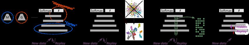
Published as a workshop paper at “Bridging AI and Cognitive Science” (ICLR 2020)

Figure 1: Overview of how current approaches of adding replay to ANNs could be mapped onto the
brain. (A) Exact or experience replay, which views the hippocampus as a memory buffer in which
experiences can simply be stored, akin to traditional views of episodic memory (Tulving, 2002; Con-
way, 2009). (B) Generative replay with a separate generative model, which views the hippocampus
as a generative neural network and replay as a generative process (Liu et al., 2018; 2019).

open problem in machine learning: acceptable performance on such problems has so far only been
achieved by methods that explicitly store data, such as iCaRL (Rebuffi et al., 2017). Here, our goal
is to find a scalable and biologically plausible way (i.e., without storing data) to make replay work
on such more realistic problems.

2   H OW DOES GENERATIVE REPLAY SCALE TO MORE COMPLEX PROBLEMS ?
To test how generative replay scales to problems with more complex inputs, we used the CIFAR-100
dataset (Krizhevsky et al., 2009) split up into 10 tasks (or episodes) with 10 classes each (Figure 2A).
It is important to note that this problem can be setup in multiple ways [or according to different
“scenarios”]. One option is that the network only needs to learn to solve each individual task,
meaning that at test time it is clear from which task an image to be classified is (i.e., the choice is
always just between 10 possible classes). This is the task-incremental learning (Task-IL) scenario
(van de Ven & Tolias, 2019) or the “multi-head” setup (Farquhar & Gal, 2018). But another, arguably
more realistic option is that the network eventually must learn to distinguish between all 100 classes.
Set up this way, it becomes a class-incremental learning (Class-IL) problem: the network must learn
a 100-way classifier, but only observes 10 classes at a time (van de Ven & Tolias, 2019). This more
challenging scenario is also referred to as the “single-head” setup (Farquhar & Gal, 2018).
On these two scenarios of split CIFAR-100, we compared the performance of generative replay (GR;
Shin et al., 2017), using a convolutional variational autoencoder (VAE; Kingma & Welling, 2013) as
generator, with that of established methods such as elastic weight consolidation (EWC; Kirkpatrick
et al., 2017), synaptic intelligence (SI; Zenke et al., 2017) and learning without forgetting (LwF;
Li & Hoiem, 2017). As baselines, we also included the naive approach of simply fine-tuning the
neural network on each new task (None; can be seen as lower bound) and a network that was always
trained using the data of all tasks so far (Joint; can be seen as upper bound). For a fair comparison,
all methods used similar-sized networks and the same training protocol (see Appendix for details).
When split CIFAR-100 was performed according to the Task-IL scenario, the methods EWC, SI and
LwF prevented catastrophic forgetting almost fully (Figure 2B). The standard version of generative
replay, however, failed on this task protocol with natural images even in the easiest scenario. When
performed according to the more realistic Class-IL scenario, the split CIFAR-100 protocol became
substantially more challenging and all compared methods (i.e., generative replay, EWC, SI and LwF)
performed very poorly suffering from severe catastrophic forgetting (Figure 2C).

3   B RAIN - INSPIRED REPLAY
The above results indicate that straight-forward implementations of generative replay break down
for more challenging problems. A likely reason is that the quality of the generated inputs that are
replayed is just too low (Figure 2D). One possible solution would be to use the recent progress in
generative modelling with deep neural networks (Goodfellow et al., 2014; van den Oord et al., 2016;
Rezende & Mohamed, 2015) to try to improve the quality of the generator. Although this approach
might work to certain extent, an issue is that incrementally training high-quality generative models is
very challenging as well (Lesort et al., 2019). Moreover, such a solution would not be very efficient,
since high-quality generative models can be computationally very costly to train and to sample from.

                                                   2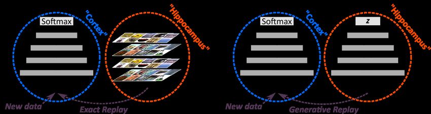
Published as a workshop paper at “Bridging AI and Cognitive Science” (ICLR 2020)
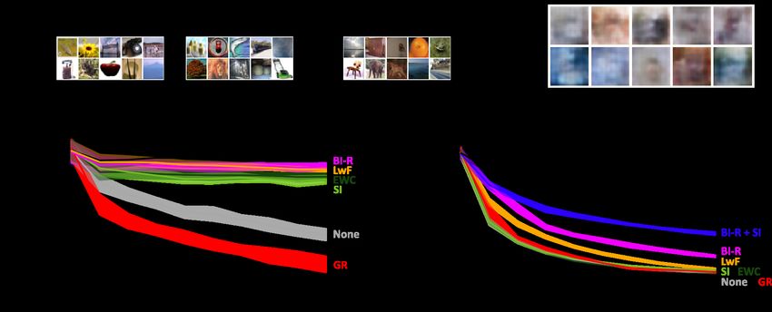
Figure 2: (A) Split CIFAR-100 performed according to two different scenarios. (B) In the Task-
IL scenario, most continual learning methods are successful, although standard generative replay
performs even worse than the naive baseline. With our brain-inspired modifications, generative re-
play outperforms the other methods. (C) In the Class-IL scenario, no existing continual learning
method that does not store data can prevent catastrophic forgetting. Our brain-inspired replay, es-
pecially when combined with SI, achieves reasonable performance on this challenging, unsolved
benchmark. (D) Examples of images replayed with standard generative replay during training on
the final task. Reported are average test accuracies based on all tasks / classes so far. Displayed are
means over 10 repetitions, shaded areas are ± 1 SEM. See main text for abbreviated method names.
Instead, we take the brain as example:
- Replay-through-feedback: For current versions of generative replay it has been suggested that
the generator, as source of the replay, is reminiscent of the hippocampus and that the main
model corresponds to the cortex (Figure 1B; Shin et al., 2017). Although this analogy
has some merit, one issue is that it ignores that the hippocampus sits atop of the cortex
in the brain’s processing hierarchy (Felleman & Van Essen, 1991). Instead, we propose
to merge the generator into the main model, by equipping it with generative backward or
feedback connections. The first few layers of the resulting model can then be interpreted as
corresponding to the early layers of the visual cortex and the top layers as corresponding to
the hippocampus (Figure 3A). We implemented this “replay-through-feedback” model as a
VAE with added softmax classification layer to the top layer of its encoder (see Appendix).
- Conditional replay: With a standard VAE, it is not possible to intentionally generate examples of
a particular class. To enable our network to control what classes to generate, we replaced
the standard normal prior over the VAE’s latent variables by a Gaussian mixture with a
separate mode for each class (Figure 3B; see Appendix). This makes it possible to generate
specific classes by restricting the sampling of the latent variables to their corresponding
modes. Additionally, for our replay-through-feedback model, such a multi-modal prior
encourages a better separation of the internal representations of different classes, as they
no longer all have to be mapped onto a single continuous distribution.
- Gating based on internal context: The brain processes stimuli differently depending on the con-
text or the task that must be performed (Kuchibhotla et al., 2017; Watanabe & Sakagami,
2007). Moreover, contextual cues (e.g., odours, sounds) can bias what memories are re-
played (Rasch et al., 2007; Rudoy et al., 2009; Bendor & Wilson, 2012). A simple but
effective way to achieve context-dependent processing in an ANN is to fully gate (or “in-
hibit”) a different, randomly selected subset of neurons in each hidden layer depending on
which task should be performed. This is the approach of context-dependent gating (Masse
et al., 2018). But an important disadvantage is that this technique can only be used when
information about context (e.g., task identity) is always available—i.e., also at test time,
which is not the case for class-incremental learning. However, we realized that in the
Class-IL scenario it is still possible to use context gates in the decoder part of our network
by conditioning on the “internal context” (Figure 3C; see Appendix). Because when pro-
ducing replay, our model controls itself from what class to generate samples, and based on
that internal decision the correct subset of neurons can be inhibited during the generative
3Published as a workshop paper at “Bridging AI and Cognitive Science” (ICLR 2020)
Figure 3: Our proposed brain-inspired modifications to the standard generative replay framework.
(A) Replay-through-feedback. The generator is merged into the main model by equipping it with
generative feedback connections (B) Conditional replay. To enable the model to generate specific
classes, the standard normal prior is replaced by a Gaussian mixture with a separate mode for each
class. (C) Gating based on internal context. For every class to be learned, a different subset of
neurons in each layer is inhibited during the generative backward pass. (D) Internal replay. Instead
of representations at the input level (e.g., pixel level), hidden or internal representations are replayed.
backward pass; while during inference (i.e., classifying new inputs) only the feedforward
layers, which are not gated, are needed.
- Internal replay: Our final modification was to replay representations of previously learned tasks
or classes not all they way to the input level (e.g., pixel level), but to replay them “inter-
nally” or at the “hidden level” (Figure 3D; see Appendix). The brain is also not thought
to replay memories all the way down to the input level. Mental images are for example
not propagated to the retina (Pearson et al., 2015). From a machine learning point of view
the hope is that generating such internal representations will be substantially easier, since
the purpose of the early layers of a neural network is to disentangle the complex input
level representations. A likely requirement for this internal replay strategy to work is that
there are no or very limited changes to the first few layers that are not being replayed.
From a neuroscience perspective this seems realistic, as for example the representations
extracted by the brain’s early visual areas are indeed not thought to drastically change in
adulthood (Smirnakis et al., 2005; Karmarkar & Dan, 2006). To simulate development, we
pre-trained the convolutional layers of our model on CIFAR-10, a dataset containing simi-
lar but non-overlapping images compared to CIFAR-100 (Krizhevsky et al., 2009). During
the incremental training on CIFAR-100, we then froze those convolutional layers and we
replayed only through the fully-connected layers. For a fair comparison, all other methods
also used pre-trained convolutional layers.
4 B RAIN - INSPIRED MODIFICATIONS ENABLE GENERATIVE REPLAY TO SCALE
To test the effectiveness of these neuroscience-inspired modifications, we applied the resulting
“brain-inspired replay” method on the same scenarios as before while using similar-sized networks.
We found that our modifications substantially improved the performance of generative replay. In the
Task-IL scenario, brain-inspired replay (BI-R) almost fully mitigated catastrophic forgetting and
outperformed EWC, SI and LwF (Figure 2B). In the Class-IL scenario, brain-inspired replay also
significantly outperformed the other methods, although its performance still remained substantially
under the “upper bound” of always training on the data of all classes so far (Figure 2C). Nevertheless,
we are not aware of any continual learning method that performs better on this challenging problem
without storing data. Finally, we found that combining our brain-inspired replay approach with SI
(BI-R + SI) substantially improved performance further, thereby further closing the gap towards the
upper bound of joint training (Figure 2C).
5 D ISCUSSION
We proposed a new, brain-inspired variant of generative replay in which internal or hidden represen-
tations are replayed that are generated by the network’s own, context-modulated feedback connec-
tions. As a machine learning contribution, our method is the first to perform well on the challenging
problem of class-incremental learning with natural images without relying on stored data. As a cog-
nitive science contribution, our method provides evidence that replay could indeed be a feasible way
for the brain to combat catastrophic forgetting.
4Published as a workshop paper at “Bridging AI and Cognitive Science” (ICLR 2020)
AUTHOR C ONTRIBUTIONS
Conceptualization, G.M.v.d.V, H.T.S. and A.S.T.; Formal analysis, G.M.v.d.V.; Funding acquisition,
A.S.T. and G.M.v.d.V.; Investigation, G.M.v.d.V.; Methodology, G.M.v.d.V.; Resources, A.S.T.;
Software, G.M.v.d.V.; Supervision, A.S.T.; Visualization, G.M.v.d.V.; Writing – original draft,
G.M.v.d.V.; Writing – review & editing, G.M.v.d.V., H.T.S. and A.S.T.
ACKNOWLEDGMENTS
We thank Mengye Ren, Zhe Li and Máté Lengyel for comments on various parts of this work, and
Johannes Oswald and Zhengwen Zeng for useful suggestions. This research project has been sup-
ported by an IBRO-ISN Research Fellowship, by the Lifelong Learning Machines (L2M) program
of the Defence Advanced Research Projects Agency (DARPA) via contract number HR0011-18-
2-0025 and by the Intelligence Advanced Research Projects Activity (IARPA) via Department of
Interior/Interior Business Center (DoI/IBC) contract number D16PC00003. Disclaimer: The views
and conclusions contained herein are those of the authors and should not be interpreted as neces-
sarily representing the official policies or endorsements, either expressed or implied, of DARPA,
IARPA, DoI/IBC, or the U.S. Government.
R EFERENCES
Rahaf Aljundi, Eugene Belilovsky, Tinne Tuytelaars, Laurent Charlin, Massimo Caccia, Min Lin,
and Lucas Page-Caccia. Online continual learning with maximal interfered retrieval. In Advances
in Neural Information Processing Systems, pp. 11849–11860, 2019.
Daniel Bendor and Matthew A Wilson. Biasing the content of hippocampal replay during sleep.
Nature Neuroscience, 15(10):1439–1447, 2012.
Martin A Conway. Episodic memories. Neuropsychologia, 47(11):2305–2313, 2009.
Carl Doersch. Tutorial on variational autoencoders. arXiv preprint arXiv:1606.05908, 2016.
Sebastian Farquhar and Yarin Gal. Towards robust evaluations of continual learning. arXiv preprint
arXiv:1805.09733, 2018.
Daniel J Felleman and David C Van Essen. Distributed hierarchical processing in the primate cere-
bral cortex. Cerebral Cortex, 1:1–47, 1991.
Robert M French. Catastrophic forgetting in connectionist networks. Trends in Cognitive Sciences,
3(4):128–135, 1999.
Ian Goodfellow, Jean Pouget-Abadie, Mehdi Mirza, Bing Xu, David Warde-Farley, Sherjil Ozair,
Aaron Courville, and Yoshua Bengio. Generative adversarial nets. In Advances in Neural Infor-
mation Processing Systems, pp. 2672–2680, 2014.
Karol Gregor, Ivo Danihelka, Alex Graves, Danilo Rezende, and Daan Wierstra. Draw: A recurrent
neural network for image generation. In International Conference on Machine Learning, pp.
1462–1471, 2015.
Geoffrey Hinton, Oriol Vinyals, and Jeff Dean. Distilling the knowledge in a neural network. arXiv
preprint arXiv:1503.02531, 2015.
Sergey Ioffe and Christian Szegedy. Batch normalization: accelerating deep network training by
reducing internal covariate shift. In International Conference on Machine Learning, pp. 448–
456, 2015.
Uma R Karmarkar and Yang Dan. Experience-dependent plasticity in adult visual cortex. Neuron,
52(4):577–585, 2006.
Diederik P Kingma and Jimmy Ba. Adam: A method for stochastic optimization. arXiv preprint
arXiv:1412.6980, 2014.
5Published as a workshop paper at “Bridging AI and Cognitive Science” (ICLR 2020)
Diederik P Kingma and Max Welling. Auto-encoding variational bayes. arXiv preprint
arXiv:1312.6114, 2013.
James Kirkpatrick, Razvan Pascanu, Neil Rabinowitz, Joel Veness, Guillaume Desjardins, Andrei A
Rusu, Kieran Milan, John Quan, Tiago Ramalho, Agnieszka Grabska-Barwinska, et al. Overcom-
ing catastrophic forgetting in neural networks. Proceedings of the National Academy of Sciences,
114(13):3521–3526, 2017.
Alex Krizhevsky, Geoffrey Hinton, et al. Learning multiple layers of features from tiny images.
Technical report, University of Toronto, 2009.
Kishore V Kuchibhotla, Jonathan V Gill, Grace W Lindsay, Eleni S Papadoyannis, Rachel E Field,
Tom A Hindmarsh Sten, Kenneth D Miller, and Robert C Froemke. Parallel processing by cortical
inhibition enables context-dependent behavior. Nature Neuroscience, 20(1):62–71, 2017.
Timothée Lesort, Hugo Caselles-Dupré, Michael Garcia-Ortiz, Andrei Stoian, and David Filliat.
Generative models from the perspective of continual learning. In International Joint Conference
on Neural Networks (IJCNN), pp. 1–8, 2019.
Zhizhong Li and Derek Hoiem. Learning without forgetting. IEEE Transactions on Pattern Analysis
and Machine Intelligence, 2017.
Kefei Liu, Jeremie Sibille, and George Dragoi. Generative predictive codes by multiplexed hip-
pocampal neuronal tuplets. Neuron, 99(6):1329–1341, 2018.
Yunzhe Liu, Raymond J Dolan, Zeb Kurth-Nelson, and Timothy EJ Behrens. Human replay spon-
taneously reorganizes experience. Cell, 178(3):640–652, 2019.
David Lopez-Paz and Marc’Aurelio Ranzato. Gradient episodic memory for continual learning. In
Advances in Neural Information Processing Systems, pp. 6467–6476, 2017.
Nicolas Y Masse, Gregory D Grant, and David J Freedman. Alleviating catastrophic forgetting
using context-dependent gating and synaptic stabilization. Proceedings of the National Academy
of Sciences, 115(44):E10467–E10475, 2018.
James L McClelland, Bruce L McNaughton, and Randall C O’Reilly. Why there are complementary
learning systems in the hippocampus and neocortex: insights from the successes and failures of
connectionist models of learning and memory. Psychological Review, 102(3):419, 1995.
Michael McCloskey and Neal J Cohen. Catastrophic interference in connectionist networks: The
sequential learning problem. In Psychology of learning and motivation, volume 24, pp. 109–165.
Elsevier, 1989.
Cuong V Nguyen, Yingzhen Li, Thang D Bui, and Richard E Turner. Variational continual
learning. In International Conference on Learning Representations, 2018. URL https:
//openreview.net/forum?id=BkQqq0gRb.
Joseph O’Neill, Barty Pleydell-Bouverie, David Dupret, and Jozsef Csicsvari. Play it again: reacti-
vation of waking experience and memory. Trends in Neurosciences, 33(5):220–229, 2010.
Joel Pearson, Thomas Naselaris, Emily A Holmes, and Stephen M Kosslyn. Mental imagery: func-
tional mechanisms and clinical applications. Trends in Cognitive Sciences, 19(10):590–602, 2015.
R Quian Quiroga, Gabriel Kreiman, Christof Koch, and Itzhak Fried. Sparse but not ‘grandmother-
cell’coding in the medial temporal lobe. Trends in Cognitive Sciences, 12(3):87–91, 2008.
Björn Rasch, Christian Büchel, Steffen Gais, and Jan Born. Odor cues during slow-wave sleep
prompt declarative memory consolidation. Science, 315(5817):1426–1429, 2007.
Roger Ratcliff. Connectionist models of recognition memory: constraints imposed by learning and
forgetting functions. Psychological Review, 97(2):285, 1990.
Sylvestre-Alvise Rebuffi, Alexander Kolesnikov, Georg Sperl, and Christoph H Lampert. icarl:
Incremental classifier and representation learning. In Conference on Computer Vision and Pattern
Recognition (CVPR), pp. 5533–5542, 2017.
6Published as a workshop paper at “Bridging AI and Cognitive Science” (ICLR 2020)
Danilo J Rezende and Shakir Mohamed. Variational inference with normalizing flows. In Interna-
tional Conference on Machine Learning, pp. 1530–1538, 2015.
Danilo Jimenez Rezende, Shakir Mohamed, and Daan Wierstra. Stochastic backpropagation and ap-
proximate inference in deep generative models. In International Conference on Machine Learn-
ing, pp. 1278–1286, 2014.
Anthony Robins. Catastrophic forgetting, rehearsal and pseudorehearsal. Connection Science, 7(2):
123–146, 1995.
David Rolnick, Arun Ahuja, Jonathan Schwarz, Timothy Lillicrap, and Gregory Wayne. Experience
replay for continual learning. In Advances in Neural Information Processing Systems, pp. 348–
358, 2019.
John D Rudoy, Joel L Voss, Carmen E Westerberg, and Ken A Paller. Strengthening individual
memories by reactivating them during sleep. Science, 326(5956):1079–1079, 2009.
Hanul Shin, Jung Kwon Lee, Jaehong Kim, and Jiwon Kim. Continual learning with deep generative
replay. In Advances in Neural Information Processing Systems, pp. 2994–3003, 2017.
Stelios M Smirnakis, Alyssa A Brewer, Michael C Schmid, Andreas S Tolias, Almut Schüz, Mark
Augath, Werner Inhoffen, Brian A Wandell, and Nikos K Logothetis. Lack of long-term cortical
reorganization after macaque retinal lesions. Nature, 435(7040):300–307, 2005.
Endel Tulving. Episodic memory: From mind to brain. Annual Review of Psychology, 53(1):1–25,
2002.
Gido M van de Ven and Andreas S Tolias. Generative replay with feedback connections as a general
strategy for continual learning. arXiv preprint arXiv:1809.10635, 2018.
Gido M van de Ven and Andreas S Tolias. Three scenarios for continual learning. arXiv preprint
arXiv:1904.07734, 2019.
Aaron van den Oord, Nal Kalchbrenner, and Koray Kavukcuoglu. Pixel recurrent neural networks.
In International Conference on Machine Learning, pp. 1747–1756, 2016.
Masataka Watanabe and Masamichi Sakagami. Integration of cognitive and motivational context
information in the primate prefrontal cortex. Cerebral Cortex, 17(suppl 1):i101–i109, 2007.
Matthew A Wilson and Bruce L McNaughton. Reactivation of hippocampal ensemble memories
during sleep. Science, 265(5172):676–679, 1994.
Matthew D Zeiler, Graham W Taylor, Rob Fergus, et al. Adaptive deconvolutional networks for mid
and high level feature learning. In International Conference on Computer Vision, pp. 2018–2025,
2011.
Friedemann Zenke, Ben Poole, and Surya Ganguli. Continual learning through synaptic intelligence.
In International Conference on Machine Learning, pp. 3987–3995, 2017.
7Published as a workshop paper at “Bridging AI and Cognitive Science” (ICLR 2020)
A PPENDIX
C ODE AVAILABILITY
Detailed, well-documented code that can be used to reproduce or build upon the re-
ported experiments will be available online at https://github.com/GMvandeVen/
brain-inspired-replay.
TASK PROTOCOL
The CIFAR-100 dataset (Krizhevsky et al., 2009) was split into ten tasks or episodes, such that each
task/episode consisted of ten classes. The original 32x32 pixel RGB-color images were normalized
(i.e., each pixel-value was subtracted by the relevant channel-wise mean and divided by the channel-
wise standard deviation, with means and standard deviations calculated over all training images), but
no other pre-processing or augmentation was performed. The standard training/test-split was used
resulting in 50,000 training images (500 per class) and 10,000 test images (100 per class).
N ETWORK ARCHITECTURE
For a fair comparison, the same base neural network architecture was used for all compared methods.
This base architecture had 5 pre-trained convolutional layers followed by 2 fully-connected layers
each containing 2000 nodes with ReLU non-linearities and a softmax output layer.
In the Task-IL scenario the softmax output layer was ‘multi-headed’, meaning that always only the
output units of classes in the task under consideration – i.e., either the current task or the replayed
task – were active; while in the Class-IL scenario the output layer was ‘single-headed’, meaning that
always all output units of the classes encountered so far were active.
The convolutional layers contained 16, 32, 64, 128 and 254 channels. Each layer used a 3x3 kernel,
a padding of 1, and a stride of 1 in the first layer (i.e., no downsampling) and a stride of 2 in the other
layers (i.e., image-size was halved in each of those layers). All convolutional layers used batch-norm
(Ioffe & Szegedy, 2015) followed by a ReLU non-linearity. For the 32x32 RGB pixel images used
in this study, these convolutional layers returned 256x2x2=1024 image features. No pooling was
used. To simulate development, the convolutional layers were pretrained on CIFAR-10, which is a
dataset containing similar but non-overlapping images and image-classes compared to CIFAR-100
(Krizhevsky et al., 2009). Pretraining was done by training the base neural network to classify the
10 classes of CIFAR-10 for 100 epochs, using the ADAM-optimizer (β1 = 0.9, β2 = 0.999) with
learning rate of 0.0001 and mini-batch size of 256.
T RAINING
The neural networks were sequentially trained on all tasks or episodes of the task protocol, with
only access to the data of the current task / episode. Each task was trained for 5000 iterations of
stochastic gradient descent using the ADAM-optimizer (β1 = 0.9, β2 = 0.999; Kingma & Ba,
2014) with learning rate of 0.0001 and a mini-batch size of 256.
G ENERATIVE REPLAY
For standard generative replay, two models were sequentially trained on all tasks: [1] the main
model, for actually solving the tasks, and [2] a separate generative model, for generating inputs
representative of previously learned tasks. See Figure 4 for a schematic.
Main model The main model was a classifier with the base neural network architecture. The loss
function used to train this model had two terms: one for the data of the current task and one for the
replayed data, with both terms weighted according to how many tasks/episodes the model had seen
so far:
1 1
Ltotal = Lcurrent + (1 − )Lreplay (1)
Ntasks so far Ntasks so far
8Published as a workshop paper at “Bridging AI and Cognitive Science” (ICLR 2020)
Figure 4: (A) Incremental training protocol with generative replay. On the first task (or episode), the
main model [M] and a separate generator [G] are trained normally. When moving on to a new task,
these two trained models first produce the samples to be replayed (see panel B). Those generated
samples are then replayed along with the training data of the current task, and both models are trained
further on this extended dataset. (B) To produce the samples to be replayed, inputs representative
of the previous tasks are first sampled from the trained generator. The generated inputs are then
labelled based on the predictions made for them by the trained main model, whereby the labels
are not simply the most likely predicted classes but vectors with the predicted probabilities for all
possible classes (i.e., distillation is used for the replay).
The loss of the current task was the standard classification loss. Because the replayed samples were
labelled with soft targets instead of hard targets, standard classification loss could not be used for
the replayed data and distillation loss was used instead (see below).
Generating a replay sample The data to be replayed was produced by first sampling inputs from
the generative model, after which those generated inputs were presented to the main model and
labelled with a target vector containing the class probabilities predicted by that model (Figure 4B).
There are however a few subtleties regarding the generation of these replay samples.
Firstly, the samples replayed during task T were generated by the versions of the generator and main
model directly after finishing training on task T − 1. Implementationally, this could be achieved
either by temporarily storing a copy of both models after finishing training on each task, or by
already generating all samples to be replayed during training on an upcoming task before training
on that task is started.
Secondly, as is common for distillation, the target probabilities predicted by the main model with
which the generated inputs were labelled were made ‘softer’ by raising the temperature T of the
softmax layer. That is, for an input x to be replayed during training of task K, the soft targets were
given by the vector ỹ with cth element equal to:
ỹc = pTθ̂(K−1) (Y = c|x) (2)
where θ̂ (K−1) is the vector with parameter values after finishing training on task K − 1 and pTθ is
the conditional probability distribution defined by the neural network with parameters θ and with
the temperature of the softmax layer raised to T . A typical value for this temperature is 2, which
was the value used here.
Thirdly, there were subtle differences between the two continual learning scenarios regarding which
output units were active when generating the soft targets for the inputs to be replayed. With the Task-
IL scenario, only the output units corresponding to the classes of the task intended to be replayed
were active (with the task intended to be replayed randomly selected among the previous tasks),
while with the Class-IL scenario the output units of the classes from up to the previously learned
task were active (i.e., classes in the current task were inactive and were thus always assigned zero
probability).
Distillation loss The training objective for replayed data with soft targets was to match the prob-
abilities predicted by the model being trained to these soft targets by minimizing the cross entropy
between them. For an input x labeled with a soft target vector ỹ, the per-sample distillation loss is
given by:
NXclasses
LD (x, ỹ; θ) = −T 2 ỹc log pTθ (Y = c|x) (3)
c=1
with temperature T again set to 2. The scaling by T 2 ensured that the relative contribution of this
objective matched that of a comparable objective with hard targets (Hinton et al., 2015).
9Published as a workshop paper at “Bridging AI and Cognitive Science” (ICLR 2020)
Generative model A symmetric variational autoencoder (VAE; Kingma & Welling, 2013;
Rezende et al., 2014) was used as generator. The VAE consisted of an encoder network qφ mapping
an input-vector x to a vector of stochastic latent variables z, and a decoder network pψ mapping
those latent variables z to a reconstructed or decoded input-vector x̃. We kept the architecture of
both networks similar to the base neural network: the encoder consisted of 5 pre-trained convolu-
tional layers (as described above) followed by 2 fully-connected layers containing 2000 ReLU units
and the decoder had 2 fully-connected layers with 2000 ReLU units followed by 5 deconvolutional
or transposed convolutional layers (Zeiler et al., 2011). Mirroring the convolutional layers, the de-
convolutional layers contained 128, 64, 32, 16 and 3 channels. The first four deconvolutional layers
used a 4x4 kernel, a padding of 1 and a stride of 2 (i.e., image-size was doubled in each of those
layers), while the final layer used a 3x3 kernel, a padding of 1 and a stride of 1 (i.e., no upsampling).
The first four deconvolutional layers used batch-norm followed by a ReLU non-linearity, while the
final layer had no non-linearity. The stochastic latent variable layer z had 100 Gaussian units (pa-
rameterized by mean µ(x) and standard deviation σ (x) , the outputs of the encoder network qφ given
input x) and the prior over them was the standard normal distribution.
Typically, the parameters of a VAE (collected here in φ and ψ) are trained by maximizing a vari-
ational lower bound on the evidence (or ELBO), which is equivalent to minimizing the following
per-sample loss function for an input x:
LG (x; φ, ψ) = Ez∼qφ (.|x) [− log pψ (x|z)] + DKL (qφ (.|x)||p(.))
(4)
= Lrecon (x; φ, ψ) + Llatent (x; φ)
2
whereby qφ (.|x) = N µ(x) , σ (x) I is the posterior distribution over the latent variables z de-
fined by the encoder given input x, p(.) = N (0, I) is the prior distribution over the latent variables
and DKL is the Kullback-Leibler divergence. With this combination of prior and posterior, it has
been shown that the “latent variable regularization term” can be calculated, without having to do
estimation, as (Kingma & Welling, 2013):
100
1 X (x) 2 (x) 2 (x) 2
Llatent (x; φ) = 1 + log(σj ) − µj − σj (5)
2 j=1
(x) (x)
whereby µj and σj are the j th elements of respectively µ(x) and σ (x) . To simplify the “recon-
struction term”, we made the output of the decoder network pψ deterministic, which is a modifica-
tion that is common in the VAE literature (Doersch, 2016; Gregor et al., 2015). We redefined the
reconstruction term as the expected binary cross entropy between the original and the decoded pixel
values:
Npixels
X
Lrecon (x; φ, ψ) = E∼N (0,I) xp log (x̃p ) + (1 − xp ) log (1 − x̃p ) (6)
p=1
whereby xp was the value of the pth pixel of the
original input image x and x̃p was the value of the
pth pixel of the decoded image x̃ = pψ z (x) with z (x) = µ(x) + σ (x) and ∼ N (0, I).
Replacing z (x) by µ(x) + σ (x) is known as the “reparameterization trick” (Kingma & Welling,
2013) and makes that a Monte Carlo estimate of the expectation in Eq. 6 is differentiable with respect
to φ. As is common in the literature, for this estimate we used just a single sample of for each
datapoint.
To train the generator, the same hyperparameters (i.e., learning rate, optimizer, iterations, batch size)
were used as for training the main model. Similar to the main model, the generator was also trained
1 1
with replay (i.e., LG G G
total = Ntasks so far Lcurrent + (1 − Ntasks so far )Lreplay ).
B RAIN - INSPIRED REPLAY
With the above described standard generative replay approach as starting point, we made the follow-
ing four modifications:
Replay-through-Feedback The “replay-through-feedback” (RtF) model was implemented as a
symmetric VAE with an added softmax classification layer to the final hidden layer of the encoder
10Published as a workshop paper at “Bridging AI and Cognitive Science” (ICLR 2020)
(i.e., the layer before the latent variable layer; Fig. 3A). Now only one model had to be trained. To
train this model, the loss function for the data of the current task had two terms that were simply
added: LRtF C G C
current = L + L , whereby L was the standard classification loss and L was the genera-
G
tive loss (see Eq. 4). For the replayed data, as for our implementation of standard generative replay,
the classification term was replaced by the distillation term from Eq. 3: LRtF D G
replay = L + L . The loss
terms for the current and replayed data were again weighted according to how many tasks/episodes
1 1
the model had seen so far: LRtF RtF RtF
total = Ntasks so far Lcurrent + (1 − Ntasks so far )Lreplay .
Conditional Replay To enable the network to generate examples of specific classes, we replaced
the standard normal prior over the stochastic latent variables z by a Gaussian mixture with a separate
mode for each class (Figure 3B):
NX
classes
pχ (.) = p(Y = c)pχ (.|c) (7)
c=1
with pχ (.|c) = N µc , σ c 2 I for c = 1, ..., Nclasses , whereby µc and σ c are the trainable mean and
standard deviation of the mode corresponding to class c, χ is the collection
of trainable means and
1
standard deviations of all classes and p(Y = c) = Categorical Nclasses is the class-prior. Because
of the change in prior distribution, the expression for analytically calculating the latent variable
regularization term Llatent in Eq. 5 is no longer valid. But for an input x labeled with a hard target
y (i.e., for current task data), because the prior distribution over the latent variables z reduces to the
mode corresponding to class y, it can be shown that Llatent still has a closed-form expression:
Llatent (x, y; φ, χ) = DKL (qφ (.|x)||pχ (.|y))
Z
qφ (z|x)
= − qφ (z|x) log dz
pχ (z|y)
= Ez∼qφ (.|x) [− log qφ (z|x)] + Ez∼qφ (.|x) [log pχ (z|y)] (8)
2
(x) 2
(x) y
J
1 X µ − µ + σ
(x) 2 y2 j j j
= 1 + log(σj ) − log(σj ) −
2 j=1 y 2
σj
whereby J is the dimensionality of the latent variables z (i.e., J = 100 for our experiments) and µyj
and σjy are the j th elements of respectively µy and σ y . The last equality is based on the following
two simplifications:
2
h i
Ez∼qφ (.|x) [− log qφ (z|x)] = Ez∼N (µ(x) ,σ(x) 2 I ) − log N z|µ(x) , σ (x) I
2
(x)
1
J z j − µj 1
J
2
(x)
X Y
J
= Ez∼N (µ(x) ,σ(x) 2 I ) + log (2π) σj
2 j=1 (x) 2 2
σj j=1
2
(x) (x) (x)
1 X µj + σj j − µj
J J
J 1X (x) 2
= E∼N (0,I) 2 + log(2π) + log σj
2 j=1 2 2 j=1
(x)
σj
J J
1X J 1X
(x) 2
= E∼N (0,1) 2 + log(2π) + log σj
2 j=1 2 2 j=1
J
1 X
(x) 2
= 1 + log(2π) + log σj
2 j=1
(9)
11Published as a workshop paper at “Bridging AI and Cognitive Science” (ICLR 2020)
h i
Ez∼qφ (.|x) [log pχ (z|y)] = Ez∼N (µ(x) ,σ(x) 2 I ) log N z|µy , σ y 2 I
2
1 XJ
zj − µyj 1 YJ
2
= Ez∼N (µ(x) ,σ(x) 2 I ) − 2
− log (2π)J σjy
2 j=1 σjy 2 j=1
2
(x) (x) y
1 X µj + σj j − µj J
J J
1X
y2
= E∼N (0,I) − 2 − log(2π) − log σ j
2 j=1 σjy 2 2 j=1
y 2 (x) 2
(x)
J
! J J
1 X µ j − µj
X σ j
X
2
=− + + J log(2π) + log σjy
2 j=1 σjy j=1 σj
y2
j=1
2
(x) y (x) 2
1 X µj − µj + σj
J
2
=− 2 + log(2π) + log σjy
2 j=1 σjy
(10)
However, for an input x labeled with a soft target ỹ (i.e., for replayed data), because the prior
distribution over the latent variables z is no a Gaussian mixture, there is no closed-form expression
for Llatent . We therefore resort to estimation by sampling, for which it is useful to express Llatent as:
Llatent (x, ỹ; φ, χ) = DKL (qφ (.|x)||pχ (.|ỹ))
Z
qφ (z|x)
= − qφ (z|x) log dz
pχ (z|ỹ)
= Ez∼qφ (.|x) [− log qφ (z|x)] + Ez∼qφ (.|x) [log pχ (z|ỹ)]
J (11)
1 X
(x) 2
= 1 + log(2π) + log σj +
2 j=1
NX
" !#
classes
c2
E∼N (0,I) log ỹc N µ(x) + σ (x) c
|µ , σ I
c=1
whereby the last equality uses Eq. 9 and the reparameterization z = µ(x) +σ (x) . Because of this
reparameterization, the Monte Carlo estimate of the final expectation in Eq. 11 is differentiable with
respect to φ.This expectation was again estimated with a single Monte Carlo sample per datapoint
(actually using the same sample as for the estimation of the expectation in Eq. 6 or Eq. 12).
When generating a sample to be replayed, the specific class y to be generated was first ran-
domly selected from the classes seen so far, after which the latent variables z were sampled from
N (µy , σ y 2 I). Although this meant that a specific class was intended to be replayed (and that class
could thus be used to label the generated sample with a hard target), it was still the case that the gen-
erated inputs were labelled with the (temperature-raised) softmax probabilities obtained for them by
a feedforward pass through the network.
Context gates To enable context-dependent processing in the generative part of our models, for
each class to be learned, a randomly selected subset of X% of the units in each hidden layer of the
decoder network was fully gated (i.e., their activations were set to zero; Figure 3C). The value of
hyperparameter X was set by a grid search (Figure 5). Note that thanks to the combination with
conditional replay, during the generation of the samples to be replayed, the specific classes selected
to be generated dictated which class-mask to use.
Internal Replay To achieve the replay of hidden or internal representations, we removed the de-
convolutational or transposed convolutional layers from the decoder network. During reconstruction
or generation, samples thus only passed through the fully-connected layers of the decoder. This
meant that replayed samples were generated at an intermediate level, and when our model encoun-
tered replayed data it let it enter the encoder network after the convolutional layers (Figure 3D).
The reconstruction term of the generative part of the loss function was therefore changed from the
12Published as a workshop paper at “Bridging AI and Cognitive Science” (ICLR 2020)
input level to the hidden level, and it was defined as the expected squared error between the hidden
activations of the original input and the corresponding hidden activations after decoding:
"N #
units 2
(x)
X
i-recon
L (x; φ, ψ) = E∼N (0,I) hi − h̃i (12)
i=1
(x)
whereby hi was the activation of the ith hidden unit when the original input image x was put
through the convolutional layers, and h̃i was the activation of the ith hidden unit after decoding
the original input: h̃ = p∗ψ z (x) with p∗ψ the decoder network without deconvolutational layers
and z (x) = µ(x) + σ (x) . The expectation in Eq. 12 was again estimated with a single Monte
Carlo sample per datapoint. To prevent large changes to the convolutional layers of the encoder, the
convolutional layers were pre-trained on CIFAR-10 (see below) and frozen during the incremental
training on CIFAR-100. For a fair comparison, pre-trained convolutional layers were used for all
compared methods.
OTHER CONTINUAL LEARNING METHODS AND BASELINES INCLUDED IN COMPARISON
SI / EWC For these methods a regularization term was added to the loss, with its strength con-
trolled by a hyperparameter: Ltotal = Lcurrent + λLregularization . The value of this hyperparameter
was set by a grid search (Figure 5). The way the regularization terms of these methods are calcu-
lated differs (Zenke et al., 2017; Kirkpatrick et al., 2017), but they both aim to penalize changes to
parameters estimated to be important for previously learned tasks.
LwF This method (Li & Hoiem, 2017) is very similar to our implementation of standard generative
replay, except that instead of using generated inputs for the replay, the inputs of the current task were
used. So there was no need to train a generator. As for our version of generative replay, these inputs
were replayed after being labeled with soft targets provided by a copy of the model stored after
finishing training on the previous task.
None As a naive baseline, the base neural network was sequentially trained on all tasks in the
standard way. This is also called fine-tuning, and can be seen as a lower bound.
Joint To get an upper bound, we sequentially trained the base neural network on all tasks while
always using the training data of all tasks so far. This is also referred to as offline training.
13Published as a workshop paper at “Bridging AI and Cognitive Science” (ICLR 2020)
Figure 5: Grid searches for EWC, SI, BI-R and BI-R + SI. Shown are the final average test set
accuracies (over all 10 tasks / based on all 100 classes) for the hyperparameter-values tested for
each method. Note that for the Task-IL scenario, combining BI-R with SI did not result in an
improvement, which is why for this scenario the performance of this combination is not reported in
the main text. For these grid searches each experiment was run once, after which 10 new runs with
different random seeds were executed using the selected hyperparameter-values to obtain the results
reported in the main text.
14You can also read