The climate impact of COVID-19-induced contrail changes - Recent
←
→
Page content transcription
If your browser does not render page correctly, please read the page content below
Atmos. Chem. Phys., 21, 9405–9416, 2021
https://doi.org/10.5194/acp-21-9405-2021
© Author(s) 2021. This work is distributed under
the Creative Commons Attribution 4.0 License.

The climate impact of COVID-19-induced contrail changes
Andrew Gettelman, Chieh-Chieh Chen, and Charles G. Bardeen
Climate and Global Dynamics and Atmospheric Chemistry, Observations and Modeling Laboratories,
National Center for Atmospheric Research, Boulder, CO, USA

Correspondence: Andrew Gettelman (andrew@ucar.edu)

Received: 9 March 2021 – Discussion started: 16 March 2021
Revised: 17 May 2021 – Accepted: 24 May 2021 – Published: 18 June 2021

Abstract. The COVID-19 pandemic caused significant eco-            1   Introduction
nomic disruption in 2020 and severely impacted air traffic.
We use a state-of-the-art Earth system model and ensembles         The COVID-19 pandemic lockdown caused lots of eco-
of tightly constrained simulations to evaluate the effect of the   nomic disruption in 2020. The reduction in greenhouse gases
reductions in aviation traffic on contrail radiative forcing and   (GHGs) and pollution (Le Quéré et al., 2020) likely impacted
climate in 2020. In the absence of any COVID-19-pandemic-          global temperatures (Forster et al., 2020). GHG reductions
caused reductions, the model simulates a contrail effective        would have resulted in cooling, and aerosol reductions would
radiative forcing (ERF) of 62 ± 59 mW m−2 (2 standard de-          have resulted in warming (Gettelman et al., 2021). One of the
viations). The contrail ERF has complex spatial and seasonal       hardest hit sectors was aviation, since it was a prime cause of
patterns that combine the offsetting effect of shortwave (so-      the rapid spread of the pandemic. Total flights dropped by
lar) cooling and longwave (infrared) heating from contrails        nearly 70 % (Fig. 1) during the height of lockdown in spring
and contrail cirrus. Cooling is larger in June–August due to       2020 and had still not recovered to their pre-pandemic levels
the preponderance of aviation in the Northern Hemisphere,          by the end of 2020.
while warming occurs throughout the year. The spatial and             Aircraft have many environmental impacts, including cli-
seasonal forcing variations also map onto surface tempera-         mate impacts. As recently reviewed by Lee et al. (2021),
ture variations. The net land surface temperature change due       global aviation warms the planet through both CO2 and
to contrails in a normal year is estimated at 0.13 ± 0.04 K        non-CO2 contributions. Global aviation contributes 3.5 % to
(2 standard deviations), with some regions warming as much         total anthropogenic radiative forcing, but non-CO2 effects
as 0.7 K. The effect of COVID-19 reductions in flight traf-        comprise about two-thirds of the net radiative forcing. The
fic decreased contrails. The unique timing of such reduc-          largest single contribution to aviation radiative forcing is
tions, which were maximum in Northern Hemisphere spring            contrails and contrail cirrus, with an estimated 2018 impact
and summer when the largest contrail cooling occurs, means         of 0.06 W m−2 (60 mW m−2 ) with high uncertainty.
that cooling due to fewer contrails in boreal spring and fall         The 2020 changes in air traffic likely resulted in reduc-
was offset by warming due to fewer contrails in boreal sum-        tions in contrail frequency (Schumann et al., 2021b). Aircraft
mer to give no significant annual averaged ERF from con-           contrails create linear condensation trails that can evolve and
trail changes in 2020. Despite no net significant global ERF,      persist in supersaturated air as contrail cirrus. Like other cir-
because of the spatial and seasonal timing of contrail ERF,        rus clouds, the resulting clouds scatter solar (shortwave –
some land regions would have cooled slightly (minimum              SW) radiation back to space, cooling the planet. Contrails
−0.2 K) but significantly from contrail changes in 2020. The       also absorb and re-emit infrared (longwave – LW) radiation
implications for future climate impacts of contrails are dis-      from the Earth at colder temperatures, warming the planet.
cussed.                                                            The net effect depends on the cirrus microphysical and radia-
                                                                   tive properties, and the variation in SW radiation. Integrating
                                                                   over space and time, the net effect of contrails is to warm
                                                                   the planet (Lee et al., 2021) through a balance of the long-
                                                                   wave (warming) and shortwave (cooling). Thus, reductions

Published by Copernicus Publications on behalf of the European Geosciences Union.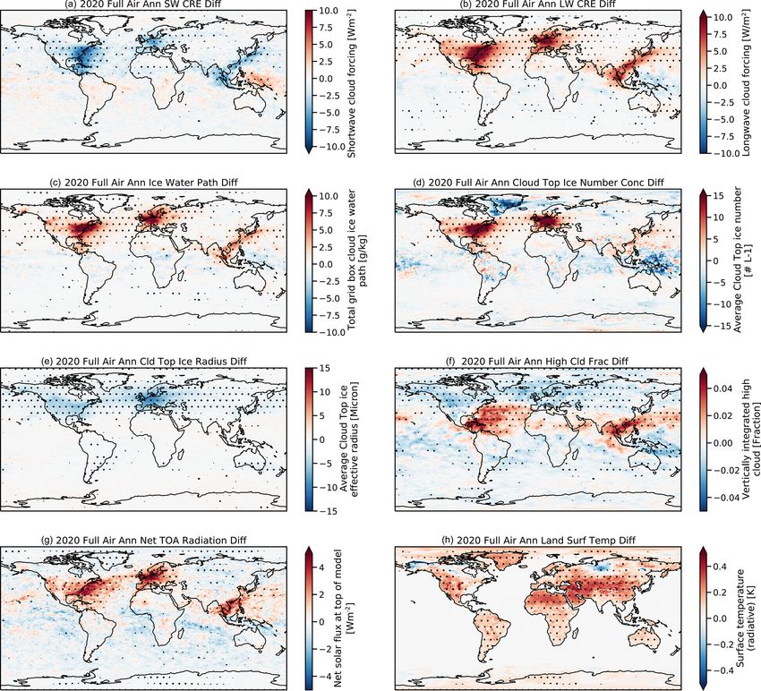
9406                                       A. Gettelman et al.: The climate impact of COVID-19-induced contrail changes

in contrails due to COVID-19 would be expected to cool the        cloud then becomes part of the model hydrologic cycle and
planet.                                                           can persist and evolve or evaporate as subsequent time steps
   This study will document the updated version of the con-       lasting from 30 min to many hours. The model can, thus, sim-
trail model that is publicly available as part of the Commu-      ulate linear contrails (representing a small cloud fraction in a
nity Earth System Model, version 2.2, and its contrail effec-     model grid box), their evolution into contrail cirrus, and their
tive radiative forcing (ERF) for a “normal” aviation in year      effect on the background environment and existing clouds.
2020 with no pandemic reductions. We then use estimates of        For this study, we focus only on the impact of aviation wa-
the changes in aviation emissions for the full year of 2020 to    ter vapor emissions. Aviation aerosols may have substantial
estimate changes in the contrail ERF due to the COVID-19          effects on subsequent cloud formation (Gettelman and Chen,
pandemic. ERF includes fast temperature adjustments due to        2013) but are highly uncertain (Lee et al., 2021), and we will
changes in cloud formation and is the usual metric for un-        focus solely on the effects of water vapor.
derstanding and assessing changes in the Earth’s radiation           For CESM, we use the standard 32 levels (to 3 hPa) ver-
budget.                                                           tical and ∼ 1◦ horizontal resolution. Winds are nudged, as
   Section 2 contains the methodology of the model and sim-       described by Gettelman et al. (2020) and Gettelman et al.
ulations, Sect. 3 contains results of the simulations, and con-   (2021). The model time step is 1800 s. Winds and op-
clusions are in Sect. 4.                                          tional temperatures are relaxed to NASA Modern-Era Ret-
                                                                  rospective analysis for Research and Applications, version 2
                                                                  (MERRA2; Molod et al., 2015), available every 3 h. The lin-
2     Model and methods                                           ear relaxation time is 24 h. CESM2 has a fully interactive
                                                                  land surface model (the Community Land Model, version 5;
2.1    Model                                                      Danabasoglu et al., 2020). Sea surface temperatures (SSTs)
                                                                  are fixed to MERRA2 SST, and there is no interactive ocean.
Simulations use the Community Earth System Model, ver-               These simulations permit temperature adjustment. Result-
sion 2 (CESM2; Danabasoglu et al., 2020). The atmospheric         ing radiative flux perturbations constitute an ERF. We also
model in CESM is the Community Atmosphere Model ver-              conduct sensitivity tests, as discussed below, where tempera-
sion 6.2 (CAM6; Gettelman et al., 2020). CAM6 uses a de-          tures are nudged to MERRA2.
tailed two-moment cloud microphysics scheme (Gettelman               We have compared the results to previous contrail simu-
and Morrison, 2015) coupled to an aerosol microphysics and        lations with this model and others, as well as with obser-
chemistry model (Liu et al., 2016), as described by Gettel-       vations. The pattern of the resulting contrail changes (illus-
man et al. (2019).                                                trated below) to cloud fraction are very similar to the pre-
   To the standard version of CESM, we add the contrail           vious model documented in CAM5 (Chen and Gettelman,
parameterization of Chen et al. (2012) that was developed         2013, their Fig. 5), with peak effects in Northern Hemi-
for CAM5. Since the ice cloud microphysics and aerosols           sphere mid-latitudes. The radiative forcing of the CAM6
are not substantially different between CAM5 and CAM6,            simulations (discussed in detail below) is larger than in
the translation is straightforward. As described by Lee et al.    (Chen and Gettelman, 2013) due to the (a) smaller (100 vs.
(2021), we adjust the assumed emission ice particle diame-        300 m) initial contrail area and (b) smaller initial ice crys-
ter to 7.5 µm from the original parameterization (10 µm) to       tal sizes (7.5 vs. 10 µm diameter). The radiative forcing pat-
better align with the observations. The representation of con-    tern and magnitude matches Bock and Burkhardt (2019, their
trails in CESM, described by Chen et al. (2012) and Chen and      Fig. 2a) qualitatively and quantitatively. This is consistent
Gettelman (2013), adds aviation emissions of water vapor. A       with the intercomparison between contrail simulation mod-
specified mass of water vapor is emitted based on a data set      els that was recently conducted as part of the review by Lee
of total aircraft distance traveled, assuming a contrail diam-    et al. (2021). The CAM6 contrail model results also compare
eter of 100 m over the grid box length and standard emis-         well to observations and simulations of contrails by Schu-
sion indices for commercial aircraft (see Chen et al., 2012       mann et al. (2021a), who analyzed differences in clouds be-
for details). If the temperature and humidity conditions indi-    tween 2020 and 2019. The CAM6 results have the same sign
cate contrail formation (Appleman, 1953; Schumann, 1996),         of cloud changes as observed and simulated in Schumann
then the vapor is converted to ice crystals with a specified      et al. (2021a). This yields further confidence in the CAM6
initial particle size of 7.5 µm (assuming small spherical ice     model estimates presented below.
crystals), yielding an ice number concentration increase. If
conditions do not imply contrail formation, then water va-        2.2   Emissions data
por is added. The vapor or ice is then is part of the fully
conservative CESM hydrologic cycle with all microphysical         To simulate aviation emissions for 2020 with and without
processes active. When ice is formed, a 100 m wide cloud          COVID changes, we modify existing aviation inventories
is added to the cloud fraction (for 100 km horizontal resolu-     used with CESM. We take the Aviation Climate Change Re-
tion, the cloud fraction added is thus 0.1 % per aircraft). The   search Initiative (ACCRI) 2006 inventory (Wilkerson et al.,

Atmos. Chem. Phys., 21, 9405–9416, 2021                                             https://doi.org/10.5194/acp-21-9405-2021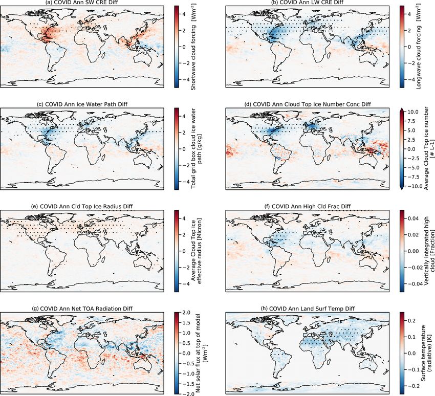
A. Gettelman et al.: The climate impact of COVID-19-induced contrail changes                                                      9407

Figure 1. (a) Daily total flights from 2016–2020. (b) Map of 2020 flight level water vapor emissions (micrograms per kilogram per day –
µg kg−1 d−1 ). (c) Monthly average flights for each year and the 2016–2019 average (thick black line). (d) Scaled weekly estimate of the
COVID-19-affected flight fraction for 2020.

2010) used with earlier versions of CESM (CAM5) (Chen                 use weekly averages, since there is a strong weekly cycle in
et al., 2012; Gettelman and Chen, 2013). We focus only on             flights (Fig. 1a). Using daily averages would have required
water vapor emissions and contrails. We do not consider               removing a weekly cycle to create scaling factors and then
the effects of aviation aerosols in this study. The ACCRI             re-imposing it and assuming it was unchanged during the
2006 inventory was developed based on detailed flight track           pandemic. The analysis yields a scaling value for every week
data. The distribution of flight level water vapor emissions          of 2020 from our reference (scaled-up 2006 emissions), as
is shown in Fig. 1b. We make the assumption that air traffic          illustrated in Fig. 1d. The first few weeks of 2020 were nor-
has increased significantly since 2006, but that the flight lo-       mal, then reductions started in February 2020, due to restric-
cations and relative density have not changed drastically. In         tions in China and Asia, and then in March (around week
some rapidly developing regions of the planet, such as China,         12) as most nations introduced a lockdown period and most
this assumption will result in some additional uncertainty.           commercial flights were halted. Total aviation declined by
   To estimate the 2020 emissions, we estimate the growth             two-thirds from what would have been expected. Recovery
in fuel use since 2006 as being equal to the growth in total          was rapid for about 10–15 weeks until the middle of 2020,
aircraft distance traveled using data from Lee et al. (2021).         and since then recovery has slowed, reaching approximately
Lee et al. (2021) report 54.7 × 10⁶ km of travel in 2018              75 %–80 % of the expected value by the end of 2020. Note
and 33.2 × 10⁶ km in 2006. The scaling from 2006 to 2018              that this value is total flights, including commercial (pas-
is then 1.58. We evaluate 2018–2020 increases in aviation             senger and cargo), private, and military (with transponders)
emissions against aircraft movement data for total (commer-           flights. The total load factor on passenger flights has de-
cial, private, and military) flights from Flightradar24 from          creased, so the total passenger miles flown is different to this.
2016–2020 (available at https://www.flightradar24.com/data/           But it is total flights that are most relevant for water vapor
statistics; last access: 15 January 2021; illustrated in Fig. 1).     emissions.
These data show growth over the last few years of 9 % per                We then have a scaling factor for 2020 from 2006 (1.88)
year. We, thus, use a 9 % per year increase over 2018–2020            and weekly modifications to that factor for COVID-19-
(2 years) to generate a scaling from 2006 to 2020 of 1.88             impacted emissions. These aviation water vapor emissions
(88 % increase from 2006) in a scenario without any COVID-            are used in our simulations to initiate contrails. All other
19-induced reductions in aviation.                                    emissions come from the Shared Socioeconomic Pathway
   In order to determine the perturbation due to the COVID-           (SSP) 245 emissions for 2019–2020 and are the same for all
19 lockdown, we use daily data for total flights for each day         simulations.
of 2020, provided by Flightradar24 and illustrated in Fig. 1a,
and compare these data to a scaled-up average of previous
years (2016–2019), which is 9 % above 2019 (Fig. 1c). We

https://doi.org/10.5194/acp-21-9405-2021                                                Atmos. Chem. Phys., 21, 9405–9416, 2021
9408                                        A. Gettelman et al.: The climate impact of COVID-19-induced contrail changes

2.3    Simulations                                                 lines; mapped to the 2020 annual cycle), which has the same
                                                                   aviation emissions but different meteorology. It is clear that
Full aviation simulations with 10 ensemble members are             the land surface temperature takes about 4 months to come
launched from 1 January 2019 to 31 December 2020                   to equilibrium with the forcing (Fig. 2h), but the other fields
(2 years), with a small temperature perturbation (10−10 K).        are all similar for all months.
The initial perturbation results in a slightly different atmo-        Aviation contrails (full air − no air) cause increases in
sphere evolution for each ensemble member. Nudging keeps           the negative SW cloud radiative effect (CRE), a net cooling
the atmosphere in a similar “weather” state. The perturba-         (Fig. 2a), and a LW CRE warming (Fig. 2b; green, orange,
tion samples random fluctuations within that state. Critically,    and purple dashed lines). The opposite effects are seen when
this enables estimates of the statistical significance of dif-     COVID-19 reductions (COVID − full Air) in contrails are as-
ferences. We compared 10 and 20 ensemble members, and              sessed (blue and red dashed lines). There is an annual cycle
found that 10 members did not change the standard deviation        in the SW CRE (Fig. 2a) with a peak cooling in the Northern
or significance levels for full aviation emissions. We define      Hemisphere (NH) summer, when maximum sunlight occurs
the statistical significance for maps with the false discovery     in the regions of maximum emissions at NH mid-latitudes.
rate (FDR) method of Wilks (2006), which reduces patterned         The LW CRE (Fig. 2b) has virtually no annual cycle. The
noise. We use the standard deviation across the ensembles          COVID-19 emissions changes should then be noted in the
to estimate uncertainty of and variability in global-averaged      context of this annual cycle. The LW CRE changes due to
quantities. A similar methodology was used to examine non-         COVID-19 reductions (Fig. 2b; blue solid and red dashed
aviation COVID-19-related aerosol emissions perturbations          lines) clearly show differences that map directly to the tem-
by Gettelman et al. (2021).                                        poral evolution of aviation reductions (Fig. 1d). The phase of
   We run simulations with full aviation water vapor emis-         the SW CRE (Fig. 2a) and LW CRE (Fig. 2b) for the COVID
sions (full air) and no aviation water vapor emissions (no         case do not exactly line up (peak SW in August; peak LW in
air). We can analyze 2019 and 2020 effects with different          April). This is because of the convolution between reductions
meteorology in the 2-year simulations. As will be noted be-        (Fig. 1d), with the peak in the SW contrail effect (Fig. 2a).
low, the land surface takes a few months to react to adjusted         The ice water path (IWP), due to full contrail effects
forcing (Fig. 2g), but the other variables adjust quickly (see     (Fig. 2c), has a small annual cycle and is similar to LW CRE
Sect. 3.1). We also run an ensemble of 20 members, restarted       (Fig. 2b), which is sensitive to ice mass. The ratio of the LW
on 1 January 2020, with COVID-19-reduced aviation water            CRE change to IWP change is similar for the 2020 full air
vapor emissions (COVID) for 2020. A total of 20 ensemble           (1.6), 2019 full air (1.6) and COVID (1.8) ensembles. There
members are used due to the smaller perturbation. Finally, we      is little change relative to the variability in global average
also run a pair of 2020 ensembles with temperature nudging         cloud top ice number (Fig. 2D), but this masks the regional
(full air T nudge; COVID T nudge) to explore how the evo-          variability which will be discussed below (Sect. 3.2). The
lution of temperature may affect the results.                      average size of ice crystals decreases due to aviation con-
                                                                   trails (Fig. 2e) and, correspondingly, increases when aviation
                                                                   contrails are reduced. This is expected as contrails add small
3     Results
                                                                   (7.5 µm initial diameter) ice crystals into the model.
First, we analyze global mean results by month in Sect. 3.1.          The changes in the high cloud (above 400 hPa) fraction
We focus on the differences between ensembles with and             are small (Fig. 2f). Few of the changes are significantly dif-
without aviation or COVID-19-affected aviation for key cli-        ferent from zero and mostly occur only in the summer pe-
mate parameters. Then we assess the spatial and seasonal dis-      riod for full aviation emissions. There is a different annual
tribution of these parameters (Sect. 3.2). This puts the overall   cycle when temperature nudging is used (Fig. 2f; purple).
global values into an important context for assessing contrail     These global changes mask the spatial and vertical structure
ERF and COVID-19 reductions in contrails. For clarity in           in cloud field changes that we will analyze in Sect. 3.3.
dates, we will refer to the COVID-19-affected aviation sim-           The top of atmosphere (TOA) radiative flux (Fig. 2g)
ulations in the figures as “COVID”. Finally, we look in more       is a residual of positive LW CRE and negative SW CRE,
detail at cloud changes and the effects of temperature nudg-       with potential additional components due to possible ef-
ing on the climate response to aviation contrails (Sect. 3.3).     fects of clouds on clear sky aerosols and surface temperature
                                                                   changes. In general, the LW CRE dominates; aviation con-
3.1    Global mean results                                         trails are a net warming effect over the annual cycle (Table 1),
                                                                   assessed at 33 or 90 mW m−2 , depending on meteorology
Figure 2 illustrates monthly global mean quantities from the       for 2020 and 2019 respectively. Combining the means and
simulations. Shaded regions are 2 standard deviations (±2σ )       standard deviations yields an estimate of 62 ± 59 mW m−2
across the ensemble. Global annual mean quantities are pro-        (±2σ range). This is very similar to the estimate from Lee
vided in Table 1. Figure 2 shows dates in 2020 but also il-        et al. (2021) for 2018. Note that the COVID-19-reduced avi-
lustrates the differences in the 2019 spin-up year (green solid    ation emissions have offsetting LW and SW effects due to

Atmos. Chem. Phys., 21, 9405–9416, 2021                                              https://doi.org/10.5194/acp-21-9405-2021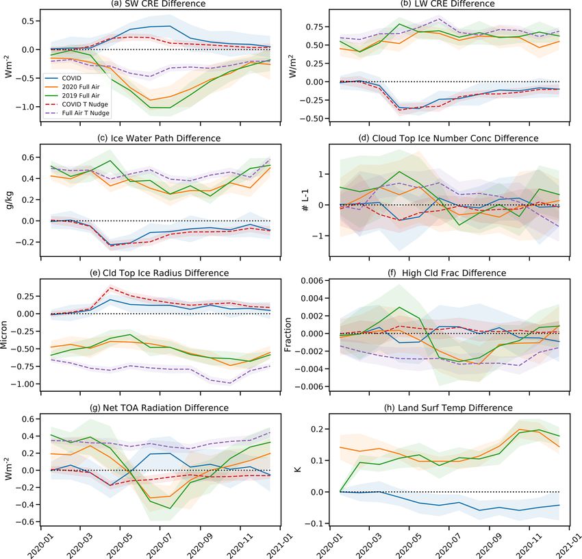
A. Gettelman et al.: The climate impact of COVID-19-induced contrail changes                                                     9409

the timing of the aviation reductions such that the net global         The result of all of these changes is significant increases in
effect is actually positive but not distinguishable from zero       TOA radiative flux (Fig. 3g) over parts of the Northern Hemi-
(27 ± 58 mW m−2 ).                                                  sphere that are in or adjacent to flight lanes. Note that there
   Even with these effects, there are very small but potentially    are some significant remote decreases in TOA flux in regions
significant changes in land surface temperature (Fig. 2h).          with decreasing high clouds and negative LW and positive
Note that, because of limited land area and seasonal evolu-         SW effects. So not only do LW and SW CRE effects of con-
tion, the land surface temperature changes may differ from          trails cancel, but there are spatial regions of increasing and
net global TOA radiation changes. Note that these simula-           decreasing TOA flux. The resulting TOA fluxes over land
tions assume zero temperature change over the ocean and,            lead to increases in land surface temperature nearly every-
thus, do not include slow ocean feedbacks. However, the ob-         where, peaking in the subtropical regions of Africa and Asia
served ocean temperatures are consistent (no additional forc-       at 0.7 K. The pattern is not dependent on specific meteorol-
ing) with full aviation effects for 2019. Since the ocean ad-       ogy; similar patterns of warming are seen in western North
justment time to any forcing is long, and the perturbations         America, subtropical Africa, the Middle East, and Asia with
are much smaller than the variability in radiative forcing, any     2019 meteorology (not shown).
imbalance due to fixed ocean temperatures should be a small            The pattern of warming is due to the seasonal cycle, illus-
effect well within the uncertainty envelope of the ensemble.        trated in Fig. 4. The lack of a significant annual mean warm-
The 2019 simulations (Fig. 2h; green line) illustrate that the      ing signal over eastern North America and reduced signal
equilibration of the land surface takes 4 months or so. Af-         over Europe is due to the seasonal cycle. There is warming
ter 4 months, the 2020 and 2019 results are nearly identi-          in winter (December–February) over Europe and moderate
cal for surface temperature. The atmospheric fields equili-         warming over the USA, with cooling at higher latitudes. In
brate much more rapidly, as seen in the similarity between          summer (June–August), however, there is significant cooling
the green (2019) and orange (2020) lines in Fig. 2a–g. The          over eastern North America and northern Europe. This arises
spatial structure will be assessed below. Thus, aviation con-       from the seasonal cycle of TOA flux (Fig. 2g), which is nega-
trails cause a significant land surface temperature warming         tive in Northern Hemisphere summer due to strong SW CRE
averaged over the “normal” (no COVID-19 reductions) 2020            cooling from contrails (Fig. 2a), while the LW warming is
annual cycle of 0.13 ± 0.04 K. The COVID-19 reductions in           more constant over the year (Fig. 2b). The TOA SW affects
aviation caused a cooling over land of −0.03 ± 0.03 K, even         land temperatures directly in the absence of clouds, while the
though there is no significant net TOA radiation difference         LW is filtered through the atmosphere; hence, the TOA net
(Fig. 2g and Table 1). This is understandable, based on the         radiation affects the surface differently in different seasons.
patterns of TOA flux, which are discussed below (Sect. 3.2).           The changes due to COVID-19 reductions in contrails
                                                                    (Fig. 5) are as expected, i.e., they are smaller and of the
3.2   Spatial patterns                                              opposite sign to the full contrail effect (Fig. 3) as contrails
                                                                    are reduced. The contour intervals in Fig. 5 are smaller than
Figure 3 illustrates the annual average spatial distribution of     Fig. 3, so some of the ensemble variability (noise) appears,
the climate quantities in Fig. 2 for the effect of full aviation    especially in the tropics (e.g., Fig. 5g). In general, similar
contrails. Stippling indicates statistical significance at the      patterns are seen in SW CRE (Fig. 5a), LW CRE (Fig. 5b),
90 % level using the FDR methodology (Wilks, 2006). The             IWP (Fig. 5c), ice number (Fig. 5d), and ice effective radius
expected pattern for many of the climate impacts matches the        (Fig. 5e). The high cloud differences are small (Fig. 5f) but
distribution of aircraft flight tracks (Fig. 1b), with peaks over   also similar and opposite to full contrail effects. There is lit-
eastern North America, Europe and Southeast and East Asia,          tle significance to annual TOA radiation changes (Fig. 5g).
as well as the North Atlantic and North Pacific oceans. A           Surface temperature over land cools as contrails are reduced
majority of the effects occur over the Northern Hemisphere.         (Fig. 5h). This has a similar and opposite pattern to the full
Contrails induce a cooling due to the SW CRE (Fig. 3a) and          contrail effects, including warming over the eastern USA and
a co-incident warming due to LW CRE (Fig. 3b). This arises          cooling over the western USA and in subtropical Africa and
due to increases in the IWP (Fig. 3c). There are significant        Asia, with the largest magnitude change −0.2 K. The cool-
regional increases in ice number concentration (Fig. 3d), not       ing is due to compensating SW and LW effects that vary by
evident in the global averages (Fig. 2d), which are concen-         season (Fig. 2).
trated where the IWP increases. The ice crystal size decreases         In all these cases, the level of significance is small, indicat-
(Fig. 3e) in a more diffuse but monotonic pattern, leading to a     ing that the signal due to COVID-19-induced changes in con-
more consistent global decrease (Fig. 2e). A high cloud frac-       trails is smaller than variability in most regions. This makes
tion has a more complex pattern of increases in the subtrop-        comparisons to observations difficult. However, recent work
ics at flight altitudes, with decreases at higher latitudes over    (Quas et al., 2021) found that in the regions of highest air
most of the Northern Hemisphere. This will be examined in           traffic density there was a 9 % decrease in expected cirrus
more detail in Sect. 3.3 together with the vertical structure of    cloud fraction in 2020. An analysis of MAM (March–May)
cloud fraction and IWP changes.                                     for high cloud coverage (Fig. 5f) shows decreases in cirrus

https://doi.org/10.5194/acp-21-9405-2021                                              Atmos. Chem. Phys., 21, 9405–9416, 2021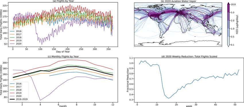
9410                                           A. Gettelman et al.: The climate impact of COVID-19-induced contrail changes

Figure 2. Global monthly mean differences between sets of ensembles. Reductions due to COVID-19 aviation changes (COVID − full air;
blue line), all aviation in 2020 (full air − no air; orange line), all aviation using 2019 meteorology (full air − no air; green line), COVID-19
changes with temperature nudging (COVID − full air; red dashed line), and full aviation with temperature nudging (full air − no air; purple
dashed line). (a) Shortwave (SW) cloud radiative effect (CRE). (b) Longwave (LW) CRE. (c) Ice water path. (d) Cloud top ice number
concentration (Cld top Ni). (e) Cloud top ice effective radius (Cld top Rei). (f) High cloud fraction (cld fract). (g) Net top of atmosphere
(TOA) radiation difference. (h) Land surface temperature difference. Shading indicates 2 standard deviations of global means across the
ensembles.

Table 1. Global annual mean differences in the fields shown in Fig. 2. Uncertainties are 2 standard deviations across each ensemble.

       Field             Units            2020 full air       2019 full air   Full air T nudge             COVID      COVID T nudge
       SW CRE            mW m−2            −446 ± 40           −471 ± 65            −290 ± 20            165 ± 47              91 ± 17
       LW CRE            mW m−2             558 ± 22            620 ± 28             675 ± 19           −153 ± 24            −171 ± 17
       TOA flux          mW m−2              33 ± 35             90 ± 50              32 ± 16             27 ± 58             −69 ± 18
       IWP               g m−2          0.36 ± 0.019        0.41 ± 0.017         0.45 ± 0.010     −0.086 ± 0.018        −0.11 ± 0.011
       Cld top Ni        L−1             0.07 ± 0.26         0.26 ± 0.29          0.20 ± 0.16      −0.032 ± 0.27       −0.150 ± 0.123
       Cld top Rei       µm            −0.52 ± 0.032       −0.53 ± 0.029        −0.79 ± 0.013      0.083 ± 0.030         0.14 ± 0.015
       High cld fract    Fraction     −0.001 ± 0.001      −0.003 ± 0.006        −0.27 ± 0.033      −0.01 ± 0.067         0.03 ± 0.035
       Land surf         K              0.134 ± 0.04        0.116 ± 0.03        −0.032 ± 0.03      −0.02 ± 0.004        0.004 ± 0.004

Atmos. Chem. Phys., 21, 9405–9416, 2021                                                       https://doi.org/10.5194/acp-21-9405-2021
A. Gettelman et al.: The climate impact of COVID-19-induced contrail changes 9411
Figure 3. Annual mean maps of differences in full air − no air for 2020. (a) Shortwave (SW) cloud radiative effect (CRE). (b) Longwave
(LW) CRE. (c) Ice water path. (d) Cloud top ice number concentration. (e) Cloud top ice effective radius. (f) High cloud fraction. (g) Net
top of atmosphere (TOA) radiation difference. (h) Land surface temperature difference. Stippled regions are significant differences using an
FDR test at 90 % confidence.
coverage up to 4 %–5 %, which is smaller than but consistent ter, results in decreasing relative humidity (not shown) and,
with observations. hence, decreases cloud fraction (Fig. 6a).
Nudging temperature alters the cloud response (Fig. 6d),
with a larger decrease in clouds at mid-latitudes and reduced
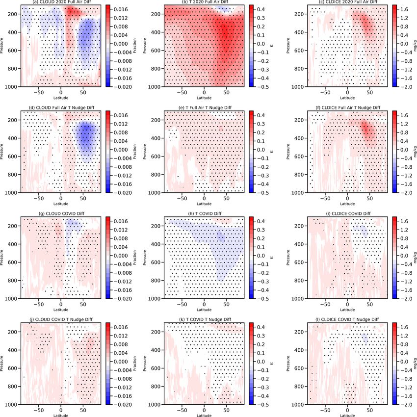
3.3 Cloud changes and effects of temperature nudging increases in cloudiness in the subtropics. The cloud ice mass
response is similar with (Fig. 6c) or without (Fig. 6f) tem-
perature nudging. The high cloud increases near the Equator
The spatial (Fig. 3f) and temporal (Fig. 2f) pattern of high
are in the subtropics and mostly zonal (Fig. 3f) and may be
cloud changes due to contrails shows significant effects
associated with temperature increases allowing more water
away from flight routes. The vertical structure of the cloud
vapor and then cloud ice to be present. This highlights the
changes, along with temperature and ice water path, are
subtle challenges of describing a radiative forcing, and why
shown in Fig. 6. Aviation water vapor causes increases in
we use ERF that includes these local temperature responses.
cloud ice mass concentrations (Fig. 6c). This can increase or
COVID-19 changes in clouds and ice without (Fig. 6g, h, j)
decrease the cloudiness (Fig. 6a) depending on the tempera-
and with (Fig. 6k, l, m) temperature nudging are similar to
ture (and humidity) response. Without temperature nudging,
full aviation effects but are smaller and of the opposite sign.
there is local warming due to LW absorption by cloud ice
(Fig. 6b). The increase in temperature and cloud ice (Fig. 6c),
some of which comes from forming contrails in supersat-
urated air and the subsequent uptake of environmental wa-
https://doi.org/10.5194/acp-21-9405-2021 Atmos. Chem. Phys., 21, 9405–9416, 20219412 A. Gettelman et al.: The climate impact of COVID-19-induced contrail changes
Figure 4. Seasonal mean maps of differences in full air − no air for 2020. The left column (a, c, e, g) shows the TOA radiation, and the
right column (b, d, f, h) shows the land surface temperature. (a, b) December–February (DJF), (c, d) March–May (MAM), (e, f) June–
August (JJA), and (g, h) September–November (SON). Stippled regions are significant differences using an FDR test at 90 % confidence.
4 Discussion and conclusions important to understand and demonstrate a significant com-
plexity in the assessment of aviation contrail impacts. This
These simulations of aviation contrails and the effect of arises because of the seasonality of SW radiation (Fig. 2a)
COVID-19-induced reductions provide some interesting mapped onto the seasonality of flights (Fig. 1), which results
new perspectives on the effect of contrails on climate. in net contrail cooling from June to September (Fig. 2g and
Contrail effective radiative forcing (ERF) is estimated at Fig. 4e) but strong global (Fig. 2g) and regional (Fig. 4a)
62 ± 59 mW m−2 (2σ ) for current (2020) aviation in the ab- heating effects in December–February. This is an underap-
sence of any COVID-19-pandemic-caused reductions. The preciated part of the contrail ERF and may have implications
variability range is due to the ensemble spread and differ- for mitigation strategies.
ences in year-to-year meteorology, indicating that the value The spatial and seasonal forcing variations also map onto
may vary from year to year. A more complete analysis of in- land surface temperature variations, resulting in smaller an-
terannual variability should be conducted but is beyond the nual temperature changes than might be expected. In western
scope of this study. This range is well in line with recent as- Europe, for example, peak net radiation differences occur in
sessments of contrail ERF (Lee et al., 2021). The specific fall and winter when radiation is a smaller part of the surface
differences between 2020 and 2019 compare well to obser- energy budget, so little temperature change results. In eastern
vations and contrail simulations of Schumann et al. (2021a). North America, the SW cooling effects of contrails dominate
The net contrail ERF has complex spatial and seasonal in spring and summer, while LW effects occur more strongly
patterns and is a residual of SW cooling and LW heating in fall and winter, such that there is little annual temperature
components nearly 10 times the net effect. The patterns are
Atmos. Chem. Phys., 21, 9405–9416, 2021 https://doi.org/10.5194/acp-21-9405-2021A. Gettelman et al.: The climate impact of COVID-19-induced contrail changes 9413 Figure 5. Annual mean maps of differences for COVID − full air for 2020. (a) Shortwave (SW) cloud radiative effect (CRE). (b) Longwave (LW) CRE. (c) Ice water path. (d) Cloud top ice number concentration. (e) Cloud top ice effective radius. (f) High cloud fraction. (g) Net top of atmosphere (TOA) radiation difference. (h) Land surface temperature difference. Stippled regions are significant differences using an FDR test at 90 % confidence. change. The largest temperature changes are found over sub- in summer, giving no significant annual averaged ERF from tropical Africa, away from flight routes, but these regions are contrail changes in 2020. Despite no net significant global perhaps affected by high cloud increase due to the remote ERF, there are some land regions that cooled significantly effects of aviation. and up to −0.2 K from what would have been expected with The temperature changes resulting from these small ERFs baseline aviation contrails. These reductions occurred in the are much smaller than climate variability in a fully coupled same regions as large contrail temperature changes in the system. For this study, ocean temperatures are fixed, which subtropical Northern Hemisphere. is fine in the short term and for small ERF estimates. With The patterns of surface warming and cooling are not ex- this caveat, there are significant increases in temperature over actly coincident with contrail ERF, indicating distributed ef- most land regions due to contrails, with an annual average fects through the climate system. These effects should be fur- over land of 0.13 ± 0.04 K. The peak annual temperature ther tested and not just with a coupled land surface (as has change is 0.7 K in the Northern Hemisphere subtropics. been done here) but with a coupled ocean. However, this will The effect of COVID-19 reductions in flight traffic introduce additional climate noise as well, so is a subject for (Fig. 1d) decreased contrails. The unique timing of such future work. reductions, which were maximum in Northern Hemisphere This study has not considered any impacts of changes to summer, when the largest contrail cooling occurs, means that aviation aerosol emissions, largely sulfate (SO4 ) and black warming reductions due to fewer contrails in the spring and carbon (BC). Aviation aerosols are highly uncertain, which fall were offset by cooling reductions due to fewer contrails is why we chose to focus on aviation water vapor. Note that https://doi.org/10.5194/acp-21-9405-2021 Atmos. Chem. Phys., 21, 9405–9416, 2021
9414                                             A. Gettelman et al.: The climate impact of COVID-19-induced contrail changes

Figure 6. Annual zonal mean latitude height plots differences in cloud fraction (a, d, g, k), temperature, T (b, e, h, l), and cloud ice mixing
ratio (c, f, j, m). The panels show COVID − full air (a, b, c), no aviation − full air (d, e, f), no aviation − full aviation T nudged (g, h, i), and
COVID − full aviation with T nudging (k, l, m). Stippled regions are significant differences using an FDR test at 90 % confidence.

aviation aerosols affect only subsequent cloud formation and                 be confirmed and are not yet quantified – even in recent as-
not initial contrails and contrail cirrus. In CESM, aviation                 sessments (Lee et al., 2021).
aerosols, especially SO4 , tend to mix downward to affect liq-                  This study provides estimates based on unique and de-
uid clouds below (Gettelman and Chen, 2013). The net effect                  tailed modeling frameworks to elucidate small changes in
of the aviation aerosols is cooling, so COVID-19 reductions                  the climate system with ensembles of constrained simula-
would likely cause a net warming. The seasonality is similar                 tions. One important question is whether any of these sim-
to the SW effects here. But these effects have not been in-                  ulated changes due to COVID-19 aviation reductions can be
cluded because there is a wide divergence in the outcomes,                   seen in observations. The pattern and timing of radiation and
depending on the model and the background state of cirrus                    warming changes might yield sufficient fingerprints in instru-
cloud microphysics. These aerosol mechanisms have yet to                     mental records of anomalies during 2020 to be able to tease
                                                                             out these effects, and this an interesting avenue for future

Atmos. Chem. Phys., 21, 9405–9416, 2021                                                          https://doi.org/10.5194/acp-21-9405-2021
A. Gettelman et al.: The climate impact of COVID-19-induced contrail changes 9415
research. Preliminary work (Quas et al., 2021) indicates ob- References
served decreases in cloud fraction in 2020 in high traffic re-
gions consistent with these simulations. This is one avenue Appleman, H. S.: The Formation of Exhaust Condensation Trails
for a comparison of these simulations to the observations. by Jet Aircraft, B. Am. Meteorol. Soc., 34, 14–20, 1953.
Bock, L. and Burkhardt, U.: Contrail cirrus radiative forcing
Other analyses are possible, and simulation results are avail-
for future air traffic, Atmos. Chem. Phys., 19, 8163–8174,
able to the community for further analysis. https://doi.org/10.5194/acp-19-8163-2019, 2019.
What does this analysis mean for the future climate im- Chen, C.-C. and Gettelman, A.: Simulated radiative forcing from
pact of contrails? The cancellation between LW and SW in- contrails and contrail cirrus, Atmos. Chem. Phys., 13, 12525–
dicates that the spatial and seasonal distribution of flights 12536, https://doi.org/10.5194/acp-13-12525-2013, 2013.
may change the contrail ERF. Local effects in space and time Chen, C. C., Gettelman, A., Craig, C., Minnis, P., and Duda, D. P.:
may not be the same as global impacts due to the timing Global Contrail Coverage Simulated by CAM5 with the Inven-
of contrails and solar insolation. If flights increase in trop- tory of 2006 Global Aircraft Emissions, J. Adv. Model. Earth Sy.,
ical regions where there is more SW radiation throughout the 4, M04003, https://doi.org/10.1029/2011MS000105, 2012.
year, this might decrease the ERF of contrails (more cool- Danabasoglu, G., Lamarque, J.-F., Bacmeister, J., Bailey, D. A.,
ing). But it also may mean more flights in regions suscepti- DuVivier, A. K., Edwards, J., Emmons, L. K., Fasullo, J., Gar-
cia, R., Gettelman, A., Hannay, C., Holland, M. M., Large,
ble to contrails, such as the upper troposphere (through re-
W. G., Lauritzen, P. H., Lawrence, D. M., Lenaerts, J. T. M.,
gions of ice supersaturation). An updated aviation emissions Lindsay, K., Lipscomb, W. H., Mills, M. J., Neale, R., Ole-
database (more recent than the scaled 2006 ACCRI inventory son, K. W., Otto-Bliesner, B., Phillips, A. S., Sacks, W., Tilmes,
used here) and projections would be useful to begin these as- S., van Kampenhout, L., Vertenstein, M., Bertini, A., Dennis,
sessments. The results here also indicate that the seasonal cy- J., Deser, C., Fischer, C., Fox-Kemper, B., Kay, J. E., Kinni-
cle could be used as a contrail mitigation strategy, whereby son, D., Kushner, P. J., Larson, V. E., Long, M. C., Mickel-
one would not want to alter or reduce contrails in regions and son, S., Moore, J. K., Nienhouse, E., Polvani, L., Rasch, P. J.,
during certain times of the year with larger SW cooling. and Strand, W. G.: The Community Earth System Model Ver-
sion 2 (CESM2), J. Adv. Model. Earth Sy., 12, e2019MS001916,
https://doi.org/10.1029/2019MS001916, 2020.
Code and data availability. Simulation output and modified code ESCOMP: CAM: The Community Atmosphere Model, GitHub,
used in this analysis are available at https://doi.org/10.5281/zenodo. available at: https://github.com/ESCOMP/CAM/tree/cam6_2_
4584078 (Gettelman, 2021). Simulations are based on CAM6.2, 022, last access: 11 June 2021.
which is available from https://github.com/ESCOMP/CAM/tree/ Forster, P. M., Forster, H. I., Evans, M. J., Gidden, M. J., Jones,
cam6_2_022 (ESCOMP, 2021). C. D., Keller, C. A., Lamboll, R. D., Quéré, C. L., Rogelj, J.,
Rosen, D., Schleussner, C.-F., Richardson, T. B., Smith, C. J.,
and Turnock, S. T.: Current and Future Global Climate Impacts
Resulting from COVID-19, Nat. Clim. Change, 10, 913–919,
Author contributions. AG designed the study, did the main simula-
https://doi.org/10.1038/s41558-020-0883-0, 2020.
tions and analysis, and wrote the paper. CCC modified the code, did
Gettelman, A.: Simulations of Contrails Under COVID-
the preliminary simulations and analysis, and helped edit the paper.
19 Effects, Zenodo [data set and code], Zenodo,
CGB assisted with the data sets and editing of the paper.
https://doi.org/10.5281/zenodo.4584078, 2021.
Gettelman, A. and Chen, C.: The Climate Impact of Avi-
ation Aerosols, Geophys. Res. Lett., 40, 2785–2789,
Competing interests. The authors declare that they have no conflict https://doi.org/10.1002/grl.50520, 2013.
of interest. Gettelman, A. and Morrison, H.: Advanced Two-Moment Bulk
Microphysics for Global Models. Part I: Off-Line Tests and
Comparison with Other Schemes, J. Climate, 28, 1268–1287,
Acknowledgements. The National Center for Atmospheric Re- https://doi.org/10.1175/JCLI-D-14-00102.1, 2015.
search is funded by the U.S. National Science Foundation. Thanks Gettelman, A., Hannay, C., Bacmeister, J. T., Neale, R. B., Pen-
to Flightradar24 for access to the total flight data. Thanks to dergrass, A. G., Danabasoglu, G., Lamarque, J.-F., Fasullo,
David S. Lee, for the discussion and analysis of aviation emissions J. T., Bailey, D. A., Lawrence, D. M., and Mills, M. J.: High
growth. Thanks also to Ulrich Schumann, for the detailed discus- Climate Sensitivity in the Community Earth System Model
sions of the recent work on observing cloud changes during 2020. Version 2 (CESM2), Geophys. Res. Lett., 46, 8329–8337,
https://doi.org/10.1029/2019GL083978, 2019.
Gettelman, A., Bardeen, C. G., McCluskey, C. S., Järvi-
Review statement. This paper was edited by Pedro Jimenez- nen, E., Stith, J., Bretherton, C., McFarquhar, G., Twohy,
Guerrero and reviewed by Donald Wuebbles and one anonymous C., D’Alessandro, J., and Wu, W.: Simulating Obser-
referee. vations of Southern Ocean Clouds and Implications for
Climate, J. Geophys. Res.-Atmos., 125, e2020JD032619,
https://doi.org/10.1029/2020JD032619, 2020.
Gettelman, A., Gagne, D. J., Chen, C.-C., Christensen, M. W., Lebo,
Z. J., Morrison, H., and Gantos, G.: Machine Learning the Warm
https://doi.org/10.5194/acp-21-9405-2021 Atmos. Chem. Phys., 21, 9405–9416, 20219416 A. Gettelman et al.: The climate impact of COVID-19-induced contrail changes Rain Process, J. Adv. Model. Earth Sy., 13, e2020MS002268, Quaas, J., Gryspeerdt, E., Vautard, R., and Boucher, O.: Climate https://doi.org/10.1029/2020MS002268, 2021. Impact of Aircraft-Induced Cirrus Assessed from Satellite Ob- Le Quéré, C., Jackson, R. B., Jones, M. W., Smith, A. J. P., Aber- servations before and during COVID-19, Environ. Res. Lett., 16, nethy, S., Andrew, R. M., De-Gol, A. J., Willis, D. R., Shan, Y., 064051, https://doi.org/10.1088/1748-9326/abf686, 2021. Canadell, J. G., Friedlingstein, P., Creutzig, F., and Peters, G. P.: Schumann, U.: On Conditions for Contrail Formation from Aircraft Temporary Reduction in Daily Global CO2 Emissions during the Exhausts (Review Article), Meteorol. Z., 5, 4–23, 1996. COVID-19 Forced Confinement, Nat. Clim. Change, 10, 647– Schumann, U., Bugliaro, L., Dörnbrack, A., Baumann, R., and 653, https://doi.org/10.1038/s41558-020-0797-x, 2020. Voigt, C.: Aviation Contrail Cirrus and Radiative Forcing Over Lee, D. S., Fahey, D. W., Skowron, A., Allen, M. R., Burkhardt, U., Europe During 6 Months of COVID-19, Geophys. Res. Lett., Chen, Q., Doherty, S. J., Freeman, S., Forster, P. M., Fuglestvedt, 48, e2021GL092771, https://doi.org/10.1029/2021GL092771, J., Gettelman, A., De León, R. R., Lim, L. L., Lund, M. T., Millar, 2021a. R. J., Owen, B., Penner, J. E., Pitari, G., Prather, M. J., Sausen, Schumann, U., Poll, I., Teoh, R., Koelle, R., Spinielli, E., Molloy, R., and Wilcox, L. J.: The Contribution of Global Aviation to An- J., Koudis, G. S., Baumann, R., Bugliaro, L., Stettler, M., and thropogenic Climate Forcing for 2000 to 2018, Atmos. Environ., Voigt, C.: Air traffic and contrail changes over Europe during 244, 117834, https://doi.org/10.1016/j.atmosenv.2020.117834, COVID-19: a model study, Atmos. Chem. Phys., 21, 7429–7450, 2021. https://doi.org/10.5194/acp-21-7429-2021, 2021b. Liu, X., Ma, P.-L., Wang, H., Tilmes, S., Singh, B., Easter, R. C., Wilkerson, J. T., Jacobson, M. Z., Malwitz, A., Balasubrama- Ghan, S. J., and Rasch, P. J.: Description and evaluation of a nian, S., Wayson, R., Fleming, G., Naiman, A. D., and Lele, new four-mode version of the Modal Aerosol Module (MAM4) S. K.: Analysis of emission data from global commercial avi- within version 5.3 of the Community Atmosphere Model, ation: 2004 and 2006, Atmos. Chem. Phys., 10, 6391–6408, Geosci. Model Dev., 9, 505–522, https://doi.org/10.5194/gmd-9- https://doi.org/10.5194/acp-10-6391-2010, 2010. 505-2016, 2016. Wilks, D. S.: On “Field Significance” and the False Dis- Molod, A., Takacs, L., Suarez, M., and Bacmeister, J.: Development covery Rate, J. Appl. Meteor. Climatol., 45, 1181–1189, of the GEOS-5 atmospheric general circulation model: evolution https://doi.org/10.1175/JAM2404.1, 2006. from MERRA to MERRA2, Geosci. Model Dev., 8, 1339–1356, https://doi.org/10.5194/gmd-8-1339-2015, 2015. Atmos. Chem. Phys., 21, 9405–9416, 2021 https://doi.org/10.5194/acp-21-9405-2021
You can also read