Experimental demonstration of a generalized Fourier's Law for non-diffusive thermal transport
←
→
Page content transcription
If your browser does not render page correctly, please read the page content below
Experimental demonstration of a generalized Fourier’s Law for
                                                                                        non-diffusive thermal transport

                                                            Chengyun Huaa ,1 Lucas Lindsay,2 Xiangwen Chen,3 and Austin J. Minnicha                3

                                                                          1
                                                                              Environmental and Transportation Science Division,
arXiv:1902.10020v1 [cond-mat.mtrl-sci] 26 Feb 2019

                                                                     Oak Ridge National Laboratory, Oak Ridge, TN 37831, USA
                                                                                    2
                                                                                        Materials Science and Technology Division,
                                                                     Oak Ridge National Laboratory, Oak Ridge, TN 37831, USA
                                                                                3
                                                                                    Division of Engineering and Applied Science,
                                                                  California Institute of Technology, Pasadena, California 91125,USA
                                                                                                (Dated: February 27, 2019)

                                                                                                       Abstract
                                                         Phonon heat conduction over length scales comparable to their mean free paths is a topic of
                                                     considerable interest for basic science and thermal management technologies. Although the failure
                                                     of Fourier’s law beyond the diffusive regime is well understood, debate exists over the proper
                                                     physical description of thermal transport in the ballistic to diffusive crossover. Here, we derive
                                                     a generalized Fourier’s law that links the heat flux and temperature fields, valid from ballistic
                                                     to diffusive regimes and for general geometries, using the Peierls-Boltzmann transport equation
                                                     within the relaxation time approximation. This generalized Fourier’s law predicts that thermal
                                                     conductivity not only becomes nonlocal at length scales smaller than phonon mean free paths,
                                                     but also requires the inclusion of an inhomogeneous nonlocal source term that has been previously
                                                     neglected. We demonstrate the validity of this generalized Fourier’s law through direct comparison
                                                     with time-domain thermoreflectance (TDTR) measurements in the nondiffusive regime without
                                                     adjustable parameters. Furthermore, we show that interpreting experimental data without this
                                                     generalized Fourier’s law leads to inaccurate measurement of thermal transport properties.

                                                     a
                                                         To whom correspondence should be addressed. E-mail: huac@ornl.gov; aminnich@caltech.edu

                                                                                                           1
I.    INTRODUCTION

     Fourier’s law fails when a temperature gradient exists over a length scale comparable
to or smaller than the mean free paths (MFPs) of heat carriers. In this regime, the heat
flux and temperature fields may differ from the predictions of heat diffusion theory based
on Fourier’s law. These discrepancies have been observed at a localized hotspot created
by a doped resistor thermometer in a suspended silicon membrane[1] and more recently in
optical pump-probe experiments including soft x-ray diffraction from nanoline arrays,[2, 3]
transient grating,[4] and thermoreflectance methods.[5–12] In particular, due to the absence
of scattering the transport properties become nonlocal, in contrast to Fourier’s law in which
the heat flux at a certain location is determined by the temperature gradient only at that
location.
     Lattice thermal transport in crystals is generally described by the Peierls-Boltzmann
equation (PBE), first derived by Peierls,[13] from which the thermal conductivity is given
in terms of the microscopic properties of phonons.[13, 14] However, solving the PBE for a
general space-time dependent problem remains a challenging task due to the high dimension-
ality of the integro-differential equation. Thus, most prior works have determined solutions
of the PBE in certain limiting cases.
     Guyer and Krumhansl[15] first performed a linear response analysis of the PBE, deriving
a space-time-dependent thermal conductivity by assuming the Normal scattering rates were
much larger than Umklapp scattering rates, and they applied their solution to develop a
phenomenological coupling between phonons and elastic dilatational fields caused by lattice
anharmonicity. Hardy and coworkers reported a rigorous quantum-mechanical formulation
of the theory of lattice thermal conductivity using a perturbation method that included
both anharmonic forces and lattice imperfections.[16–18] This quantum treatment of lattice
dynamics was then verified by both theoretically and experimentally demonstrating the
presence of Poiseuille flow and the second sound in a phonon gas at low temperatures when
Umklapp processes may be neglected.[19–23] The variational principle was also used to
solve the PBE with Umklapp scattering incorporated.[24, 25] Levinson developed a nonlocal
diffusion theory of thermal conductivity from a solution of the PBE with three-phonon
scattering in the low frequency limit.[26]
     Advances in computing power have enabled the numerical solution of the PBE with

                                             2
inputs from density functional theory, fully ab initio. For instance, bulk lattice thermal
conductivities are now routinely computed from first principles using an iterative solution of
the PBE[27–31] or from variational approaches.[32] Chaput[33] presented a direct solution
to the transient linearized PBE with an imposed constant temperature gradient. Cepellotti
and Marzari[34] introduced the concept of a ”relaxon”, an eigenstate of the symmetrized
scattering operator of the PBE first used by Guyer et. al.[15] and Hardy[21]. They applied
this treatment to solve steady-state problems in two-dimensional systems with a constant
temperature gradient imposed in one direction[35].
   Solving the PBE with the full collision operator, even in its linearized form, is diffi-
cult for complicated geometries. Therefore, various theoretical frameworks based on a
simplified PBE have been developed to describe nonlocal thermal transport for general
problems. Non-diffusive responses observed in experiments[4–6, 8, 36, 37] have been ex-
plained using the phonon-hydrodynamic heat equation[38], a truncated Levy formalism[39],
a two-channel model in which low and high frequency phonons are described by the PBE
and heat equation[40], and a Mckelvey-Shockley flux method[41]. Methods based on solv-
ing the PBE under the relaxation time approximation (RTA), where each phonon mode
relaxes towards thermal equilibrium at a characteristic relaxation rate, have been devel-
oped to investigate nonlocal transport in an infinite domain[42–45], a finite one-dimensional
slab[46, 47], and experimental configurations such as transient grating[45, 48] and thermore-
flectance experiments[49–51]. An efficient Monte Carlo scheme has been used to solve the
PBE under the RTA in complicated geometries involving multiple boundaries[52–54].
   In the diffusion regime, Fourier’s law is a relation between heat flux and temperature
fields, independent of the specific problem. In the nondiffusive regime, obtaining such a
relation is more complicated because the transport is inherently nonlocal. The works de-
scribed above solve the PBE for problems with specific boundary conditions or inputs. Thus,
despite these efforts, a description generalizing Fourier’s law for arbitrary geometries and
linking the heat flux and temperature fields in all transport regimes is not available.
   Here, we derive a generalized Fourier’s law to describe non-diffusive thermal transport
for general geometries using the linearized PBE within the RTA. The generalized Fourier’s
law requires the inclusion of an inhomogeneous nonlocal term arising from the source or the
boundary conditions of the particular problem. By including the inhomogeneous contribu-
tion to the heat flux, the space- and time-dependent thermal conductivity is independent

                                             3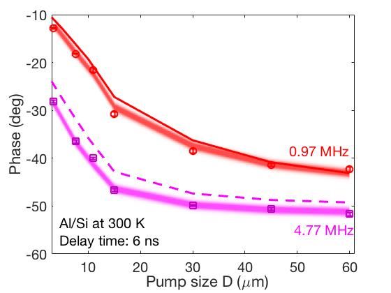
of the specific geometry or inputs. This generalized Fourier’s law is validated by favorable
comparisons with a series of TDTR measurements in the non-diffusive regime. We also show
that neglecting the inhomogeneous contribution to the heat flux leads to inaccurate mea-
surement of thermal transport properties in the non-diffusive regime. Our work provides a
unified description of heat transport for a wide range of problems from ballistic to diffusive
regimes.

II.     THEORY

      A.   Governing Equation

      We begin by briefly reviewing the derivation of the transport solution to the PBE. The
mode-dependent PBE under the relaxation time approximation for transport is given by
                  ∂gµ (x, t)                       gµ (x, t) − g0 (T (x, t))
                             + vµ · ∇gµ (x, t) = −                           + Q̇µ (x, t),    (1)
                     ∂t                                       τµ
where gµ (x, t) = ~ωµ (fµ (x, t) − f0 (T0 )) is the deviational energy distribution function at
position x and time t for phonon states µ (µ ≡ (q, s), where q is the wavevector and s is the
phonon branch index). f0 is the equilibrium Bose-Einstein distribution, and g0 (T (x, t)) =
~ωµ (f0 (T (x, t)) − f0 (T0 )) ≈ Cµ ∆T (x, t), where T (x, t) is the local temperature, T0 is the
global equilibrium temperature, ∆T (x, t) = T (x, t) − T0 is the local temperature deviation
from the equilibrium value, and Cµ = ~ωµ ∂f 0
                                         ∂T T0
                                              | is the mode-dependent specific heat. Here,
we assume that ∆T (x, t) is small such that g0 (T (x, t)) is approximated to be the first
term of its Taylor expansion around T0 . Finally, Q̇µ (x, t) is the heat input rate per mode,
vµ = (vµx , vµy , vµz ) is the phonon group velocity vector, and τµ is the phonon relaxation
time.
      To close the problem, energy conservation is used to relate gµ (x, t) to ∆T (x, t) as
                                   ∂E(x, t)
                                            + ∇ · q(x, t) = Q̇(x, t),                         (2)
                                     ∂t
where E(x, t) = V −1       gµ (x, t) is the total volumetric energy, q(x, t) = V −1 µ gµ (x, t)vµ
                         P                                                         P
                             µ

is the directional heat flux, and Q̇(x, t) = V −1 µ Q̇µ (x, t) is the volumetric mode-specific
                                                     P

heat input rate. Here, the sum over µ denotes a sum over all phonon modes in the Brillouin
zone, and V is the volume of the crystal. The solution of Eq. (1) yields a distribution
function, gµ (x, t), from which temperature and heat flux fields can be obtained using Eq. (2).

                                                   4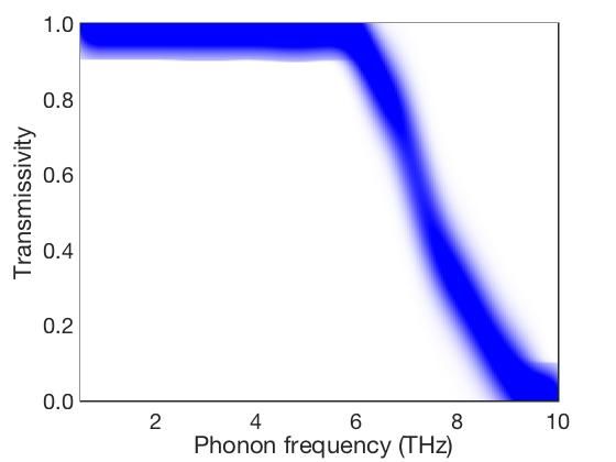
Like the classical diffusion case, the exact expression of the temperature field varies from
problem to problem. However, in a diffusion problem, the constitutive law that links the
temperature and heat flux fields is governed by one expression, Fourier’s law. Here, we
seek to identify a similar relation that directly links temperature and heat flux fields for
non-diffusive transport, regardless of the specific problem.
   To obtain this relation, we begin by rearranging Eq. (1) and performing a Fourier trans-
form in time t on Eq. (1), which gives
                      ∂g̃µ       ∂g̃µ       ∂g̃µ
                Λµx        + Λµy      + Λµz      + (1 + iητµ )g̃µ = Cµ ∆T̃ + Q̃µ τµ ,              (3)
                      ∂x         ∂y         ∂z
where η is the Fourier temporal frequency, and Λµx , Λµy and Λµz are the directional mean
free paths along x, y, and z directions, respectively. Equation (3) can be solved by defining
a new set of independent variables ξ, ρ, and ζ such that

                                            ξ = x,                                                (4a)
                                                Λµy         Λµx
                                            ρ=      x−          y,                                (4b)
                                                 Λµ         Λµ
                                                Λµz         Λµx
                                            ζ=      x−          z,                                (4c)
                                                 Λµ         Λµ
              Λµx + Λ2µy + Λ2µz . The Jacobian of this transformation is Λ2µx /Λ2µ , a nonzero
             p 2
where Λµ =
value. After changing the coordinates from (x, y, z) to the new coordinate system (ξ, ρ, ζ),
(vµξ = vµx , 0, 0) is the set of elements for the velocity vector vµ in the new coordinates, and
Eq. (3) becomes a first order partial differential equation with only one partial derivative
                                       ∂g̃µ
                                 Λµξ        + αµ g̃µ = Cµ ∆T̃ + Q̃µ τµ ,                           (5)
                                       ∂ξ
where αµ = 1 + iητµ . Assuming that ξ ∈ [L1 , L2 ], Eq. (5) has the following solution:
                                            Z ξ                          0
                                     ξ−L1
                              + −αµ Λµξ          Cµ ∆T̃ + Q̃µ τµ −αµ ξ−ξ
         g̃µ (ξ, ρ, ζ, η) = Pµ e          +                     e     Λµξ
                                                                           dξ 0 for vµξ > 0,      (6a)
                                              L1      Λµξ
                                    L2 −ξ
                                           Z L2                          0
                                 αµ              Cµ ∆T̃ + Q̃µ τµ −αµ ξ−ξ
         g̃µ (ξ, ρ, ζ, η) = Pµ− e Λµξ −                         e    Λµξ
                                                                           dξ 0 for vµξ < 0.      (6b)
                                            ξ         Λ µξ

Pµ+ and Pµ− are functions of ρ, ζ, η and are determined by the boundary conditions at ξ = L1
and ξ = L2 , respectively. Using the symmetry of vµξ about the center of the Brillouin zone,
i.e., vµξ = −v−µξ , Eqs. (6a) & (6b) can be combined into the following form:
                                                                                 ξ0 −ξ
                                                       Z
                                         −αµ Λξ            Cµ ∆T̃ + Q̃µ τµ −αµ
                  g̃µ (ξ, ρ, ζ, η) = Pµ e     µξ   +                      e      Λµξ
                                                                                         dξ 0 ,    (7)
                                                       Γ       |Λµξ |

                                                   5
where L
P + eαµ Λµξ1 if vµξ > 0
µ
Pµ = L
αµ Λ 2
(8)
P −e µξ if vµξ < 0
µ
and
[L , ξ) if v > 0
1 µξ
Γ∈ . (9)
(ξ, L2 ] if vµξ < 0
The energy conservation equation becomes
X ∂g̃µ X X
vµξ + iη g̃µ = Q̃µ , (10)
µ
∂ξ µ µ
where vµξ g̃µ gives the mode-specific heat flux along the ξ direction expressed as:
ξ−ξ0 ξ−ξ0
Z Z
−αµ Λξ 0 −αµ 0 Cµ vµξ −αµ
q̃µξ = Pµ vµξ e µξ + Q̃µ (ξ , ρ, ζ, η)e Λµξ
dξ + ∆T̃ (ξ 0 , ρ, ζ, η)e Λµξ
dξ 0 .
Γ Γ |Λµξ |
(11)
Applying integration by parts to the third term in Eq. (11), we can write the heat flux
per mode as:
Z
∂ T̃ 0
q̃µξ = − κµξ (ξ − ξ 0 ) dξ + Bµ (ξ, ρ, ζ, η), (12)
Γ ∂ξ 0
where
0
−αµ Λξ Cµ |vµξ | −αµ Λµξ
ξ
αµ Λξ
Bµ (ξ, ρ, ζ, η) = Pµ vµξ e µξ + e ∆T̃ e µξ
αµ Γ
ξ−ξ0
Z
0 −αµ
+ sgn(vµξ ) Q̃µ (ξ , ρ, ζ, η)e Λµξ
dξ 0 , (13)
Γ
is solely determined by the boundary condition and the volumetric heat input rate. κµξ (ξ)
is the modal thermal conductivity along the ξ direction given by
ξ
Λµξ
−αµ
e
κµξ (ξ) = Cµ vµξ Λµξ . (14)
αµ |Λµξ |
Equation (12) is the primary result of this work. This equation links temperature gradient
to the mode-specific heat flux for a general geometry. Since this constitutive equation of heat
conduction is valid from ballistic to diffusive regimes, we denote it as a generalized Fourier’s
law. It describes that for a specific phonon mode µ, heat only flows in the ξ direction in
the new coordinate system (ξ, ρ, ζ) since the velocities in ρ and ζ directions are zero. To
obtain the total heat flux in the original coordinate system, e.g. qx , qy , and qz in Cartesian
coordinates, all the functions involved in Eq. (12) must be mapped from the coordinate
6system (ξ, ρ, ζ) to (x, y, z). Analytical mappings exist for a few special cases that we will
discuss shortly.
There are two parts in Eq. (12). The first part represents a convolution between the
temperature gradient along the ξ direction and a space-and time-dependent thermal con-
ductivity, κµξ (ξ). As reported previously, this convolution indicates the nonlocality of the
thermal conductivity.[42, 44, 47] However, a second term exists that is determined by the
inhomogeneous term originating from the boundary conditions and source terms. Sim-
ilar to the first term, the contribution from the heat input to the heat flux, given by
0
−αµ ξ−ξ
0
R Λµξ
Q̃ (ξ , ρ, ζ, η)e
Γ µ
dξ, is nonlocal, meaning the contribution at a given point is de-
termined by convolving the heat source function with an exponential decay function with a
decay length of Λµx .
While the nonlocality of thermal conductivity was identified by earlier works on phonon
transport[6, 15, 20, 26, 39, 42, 44, 55], the contribution from the inhomogeneous term has
been neglected. Recently, Allen and Perebeinos[44] considered the effects of external heating
and derived a thermal susceptibility based on the PBE that links external heat input to
temperature response and a thermal conductivity that links temperature response to heat
flux. However, their derived thermal susceptibilities and thermal conductivities are subject
to the specific choice of the external heat input. In this work, we demonstrate that there
exists a general relation between heat flux and temperature distribution without specifying
the geometry of the problem. The space- and time-dependent thermal conductivity in the
first term of Eq. (12) is independent of boundary conditions and heat input. The dependence
of heat flux on the specific problem is accounted for by the inhomogeneous term.
B. Diffusive limit
Here we examine some specific limits of Eq. (12). First, in the diffusive regime, the
spatial and temporal dependence of thermal conductivity disappears and asymptotically
approaches a constant. To demonstrate this limit, we first identify two key nondimensional
parameters in Eq. (12): Knudsen number, Knµ ≡ Λµξ ξ −1 , which compares phonon MFP
with a characteristic length, in this case ξ −1 , and a transient number, Ξµ ≡ ητµ , which
compares the phonon relaxation times with a characteristic time, in this case η −1 . In the
diffusive limit, both Ξ and Kn are much less than unity. Then, Eq. (7) is simplified to
7Cµ ∆T̃ , and Eq. (12) becomes
Z
∂ T̃ 0 0 ∂ T̃
q̃µξ = − Cµ vµξ Λµξ δ(ξ − ξ )dξ = −κµξ , (15)
Γ ∂ξ 0 ∂ξ
since in this limit we can perform the following simplifications
lim αµ ≈ 1, (16)
Ξ→0
−αµ |Λξ
lim e µξ | ≈ 0, (17)
Ξ, Kn→0
ξ−ξ0
−αµ Λµξ
e
lim ≈ δ(ξ − ξ 0 ). (18)
Ξ, Kn→0 |Λµx |
The equation of energy conservation becomes
X ∂ 2 T̃ X X
− κµξ + iη C µ ∆T̃ = Q̃µ . (19)
µ
∂ξ 2 µ µ
∂ ∂ ∂ Λµy ∂ Λµz
Since ∂ξ
= ∂x
+ ∂y Λµx
+ ∂z Λµx
, Eq. (19) can be mapped back to Cartesian coordinates as
∂ 2 T̃ ∂ 2 T̃ ∂ 2 T̃ X X
κx + κy + κz + iη∆T̃ C µ = Q̃µ , (20)
∂x2 ∂y 2 ∂z 2 µ µ
P
where κi = µ Cµ vµi Λµi is the thermal conductivity along axis i = x, y, or z. Here, we
assume that the off-diagonal elements of the thermal conductivity tensor are zero, i.e.,
P
κij = µ Cµ vµi Λµj = 0 when i 6= j. Equation (20) is the classical heat diffusion equation.
C. Generalized Fourier’s law in a transient grating experiment
We now check another special case of Eq. (12) by applying it to the geometry of a one-
dimensional transient grating experiment.[4, 56] Since it is a 1D problem, ξ in Eq. (12) is
equivalent to x. In this experiment, the heat input has a spatial profile of eiβx in an infinite
domain, where β ≡ 2π/L and L is the grating period. The boundary term vanishes, i.e.,
ξ ∈ (−∞, ∞), and both the distribution function and temperature field exhibit the same
spatial dependence. Then, the total heat flux is expressed as
X κµx X Qµ eiβx αµ Λµx
q̃x (x, η) = iβ T̃ (η)eiβx 2 + Λ2 β 2
+ 2 + Λ2 β 2
, (21)
µx>0
α µ µx µx>0
δ αµ µx
8P
where the total volumetric energy deposited on a sample is given by µ Qµ , and the duration
of the energy deposition is δ. A derivation of Eq. (21) is given in Appendix A.
The time scale of a typical TG experiment is on the order of a few hundred nanoseconds
while relaxation times of phonons are typically less than a nanosecond for many semicon-
ductors at room temperature. Therefore, we assume that Ξ
1, and Eq. (21) is simplified
to
X κµx X Qµ eiβx Λµx
q̃x (x, η) = iβ T̃ (η)eiβx 2 β2
+ 2 β2
. (22)
µx >0
1 + Λ µx µ >0
δ 1 + Λ µx
x
which is consistent with what has been derived in our earlier work.[40, 56] The first part of
Eq. (22) represents the conventional understanding of nonlocal thermal transport, a Fourier
type relation with a reduced thermal conductivity given by
X κµx
κx = , (23)
µx >0
1 + Λ2µx β 2
while the second part of the equation represents the contribution from the heat source to
the total heat flux, which increases as the Knudsen number Λµx /L increases. In a TG
experiment, the presence of a single spatial frequency simplifies the convolutions in Eq. (12)
into products, and the only time dependence comes from the temperature. Therefore, the
decay rate of the measured transient temperature profile is directly proportional to the
reduced thermal conductivity. In general, the spatial dependency of the temperature field
is less complicated in a TG experiment than in other experiments, making the separation of
the intrinsic thermal conductivity contribution from the inhomogeneous contribution easier.
D. Generalized Fourier’s law with infinite transverse geometries
The third special case considered here is when the y and z directions extend to infinity.
The analytical mapping of Eq. (12) to Cartesian coordinates can be completed via Fourier
transform in y and z. After Fourier transform, Eq. (12) becomes
Z L2
∂T X
q̃x (x, fy , fz , η) = − κx (x − x0 , fy , fz , η) 0 dx0 + B̃µ (x, fy , fz , η), (24)
L1 ∂x µ
where thermal conductivity κx is given by
1+iΞµ +ify Λµy +ifz Λµz
− x
X e |Λµx |
κx (x, fy , fz , η) = κµx . (25)
µx >0,µy ,µz
(1 + iΞµ + ify Λµy + ifz Λµz )|Λµx |
9fy and fz are the Fourier variables in the y and z directions, correspondingly, and B̃µ (x, fy , fz , η)
is the Fourier transform of Bµ (x, ρ, ζ, η) with respect to fy and fz . The exact expression of
B̃µ and a derivation of Eq. (24) are given in Appendix B. In this case, both temperature
field and the inhomogeneous term have spatial and temporal dependence. Their dependence
on the boundary conditions and heat source should be accounted for when extracting the
intrinsic thermal conductivity from the observables such as total heat flux or an average
temperature.
III. RESULTS
We now experimentally validate the generalized Fourier’s law by comparing the predicted
and measured surface thermal responses to incident heat fluxes in TDTR experiments. We
consider a sample consisting of an aluminum film on a silicon substrate. Phonon dispersions
for Al and Si and lifetimes for Si were obtained from first-principles using density functional
theory (DFT).[57] We assumed a constant MFP for all modes in Al; the value ΛAl = 60 nm
is chosen to yield a lattice thermal conductivity κ ≈ 123 Wm−1 K−1 so that no size effects
occur in the thin film. The justification of such an approach can be found in Ref. [11].
In a TDTR experiment, the in-plane directions are regarded as infinite, thus Fourier
transforms in the y and z directions are justified. The cross-plane direction in the substrate
layer is semi-infinite. Therefore, the cross-plane heat flux in the substrate is described by
Eq. (24) with x ∈ [0, ∞). Pµ+ in Eq. (8) is determined by the interface conditions.[11]
In the diffusion regime, energy conservation, Fourier’s law and the boundary conditions
can fully describe a transport problem. In the nondiffusive regime, the replacement of
Fourier’s law is the generalized Fourier’s law described in this work. If validated, this
methodology allows the full prediction of the surface response for the wide variety of param-
eters employed in TDTR experiments, e.g., heating geometry, modulation frequency, and
temperature.
To validate this methodology, we compare the calculated TDTR responses using the
generalized Fourier’s law with pump-size-dependent TDTR measurements on the same Al/Si
sample measured in Ref. [11], where the 1/e2 diameter D of a Gaussian pump beam was
varied between 5 to 60 µm at different temperatures. As the pump size decreases and
becomes comparable to the thermal penetration depth along the cross-plane direction (x-axis
10of the schematic in Fig. 1(a)), in-plane thermal transport is no longer negligible and requires
a three-dimensional transport description. Pµ+ (ξy , ξz , η) is determined from the interface
condition, and for a given ξy , ξz , and η it is determined by the spectral transmissivity of
phonons as given in Ref. [11]. In the same work[11], we have already used the PBE within the
RTA to model the one-dimensional (ξy = ξz = 0) thermal transport in a TDTR experiment
with a uniform film heating and developed a method to extract the spectral transmissivity
profile of phonons from measurements. We also provided evidence that elastic transmission of
phonons across an interface was the dominant energy transmission mechanism for materials
with similar phonon frequencies. Therefore, the measured transmissivity profile at room
temperature given in Ref. [11] should be able to fully describe the interface conditions at
other temperatures, and there are no adjustable parameters in the present simulations.
We compared the measured signals directly to predictions from the nonlocal transport
governed by the generalized Fourier’s law and the strictly diffusive transport governed by
Fourier’s law. To ensure a consistent comparison between the constitutive relations, the
thermal conductivity of silicon is obtained using the same DFT calculations, and the interface
conductance G is given by[58]
1 4 2 2
= P Si Si − P Al Al − P Si Si (26)
G µ Cµ vµ TSi→Al µ Cµ vµ µ Cµ vµ
where TSi→Al is the phonon transmissivity from Si to Al. This expression was first derived
by Chen and Zeng, which considers the non-equilibrium nature of phonon transport at the
interface within the phonon transmissivity.[58]
Figures 1 (a) & (b) show the total signal versus delay time with a pump size of 15 µm at
room temperature for the experiments and predictions from the generalized Fourier’s law and
original Fourier’s law. As in Ref. [11], the intensity of the shaded regions correspond to the
likelihood of the measured transmissivity profile plotted in the inset of Fig. 1(b). A higher
likelihood of a transmissivity profile is indicated by a higher intensity of the shaded area,
and thus the PBE simulation using a transmissivity profile with higher likelihood better fits
the experimentally measured TDTR signals. Excellent agreement between predictions from
the generalized Fourier’s law and experiments are observed. On the other hand, Fourier’s
law fails to accurately account for the experimental data, overestimating the phase and
underestimating the amplitude after 2 ns in delay time. Note that the different transmissivity
profiles in the inset of Fig. 1(b) give a value of interface conductance G = 223±10 Wm−2 K−1
11a) D b)
z Al
y
x
Substrate
Measured TSi->Al in Ref. 11
FIG. 1. Experimental TDTR data (symbols) on the Al/Si sample with a pump beam size of 15
µm at T = 300 K for modulation frequencies of 0.97 MHz and 4.77 MHz along with the (a) ampli-
tude and (b) phase compared with predictions from the generalized Fourier’s law (shaded regions)
and original Fourier’s law (curves). The shaded regions around the PBE simulations correspond
to the likelihood of the measured transmissivity possessing a particular value (darker area corre-
sponds to more probable). Using the measured transmissivity profile from uniform heating,[11]
the prediction from the generalized Fourier’s law agrees well with the TDTR measurements, while
the Fourier results overestimate the phase and underestimate the amplitude at later times. Inset
in (a): schematic of the sample subject to a Gaussian beam heating. Inset in (b): the measured
transmissivity of longitudinal phonons TSi→Al (ω) that is obtained under a uniform film heating in
Ref. [11].
using Eq. (26), and this deviation in G leads to uncertainties in the TDTR signals that are
within the linewidth of the plotted curves.
In Figs. 2(a) & (b), comparisons of phases at different pump sizes between the generalized
Fourier’s law, original Fourier’s law and experimental data are given at 300 K. In Figs. 2(c)
& (d), we compare the measured phase versus modulation frequency at a fixed pump size
to predictions from the generalized Fourier’s law and original Fourier’s law at 100, 150, 200,
250 K. The data are given for two different delay times, 1.5 ns and 6 ns. The figure shows
that predictions from the original Fourier’s law do not reproduce the experimental results.
The deviation of Fourier’s law predictions from the experimental results becomes larger
12a) b) D
z Al
y
x
Substrate
c) d)
FIG. 2. Measured and predicted phases versus pump size at room temperature and a fixed delay
time of (c) 1.5 ns and (d) 6 ns for modulation frequencies of 0.97 MHz and 4.77 MHz. At temper-
atures of 100, 150, 200, and 250 K, measured and predicted phases are plotted versus modulation
frequency at a fixed delay time of (c) 1.5 ns and (d) 6 ns for a pump size of 15 µm. The symbols are
TDTR data and the shaded regions are predictions. The curves show the prediction by Fourier’s
law with temperature-dependent thermal conductivities from DFT and the interface conductance
given by Eq. (26).
when the temperature decreases, modulation frequency increases, or pump size decreases,
all indicating that non-diffusive effects increase with these changes. On the other hand, pre-
dictions from the generalized Fourier’s law agree well with the experimental measurements
13a) 0.35 LA Profile 1:
c) 1.2
Thermal conductivity (Wm K )
G = 115 MWm-2K-1 Profile 2
-1
Transmissivity
0.25 TA
-1
TA 1.1
0.15 Profile 1
0.05 1.0
0 2 4 6 8 10
Phonon frequency (THz)
b) 0.7 Profile 2:
0.9
LA
G = 253 MWm-2K-1 D
Transmissivity
TA
0.5
Al 0.51 MHz
TA 0.8
0.3 5.52 MHz
BAs at 300 K 10.1 MHz
0.1 0.7
5 10 20 30 40 50 60
0 2 4 6 8 10
Phonon frequency (THz) Pump diameter ( m)
FIG. 3. Spectral transmissivity profiles from BAs to Al versus phonon frequency that give an
interface conductance of (a) 115 MWm−2 K−1 and (b) 253 MWm−2 K−1 using Eq. (26). The
profiles are used to generate the synthetic TDTR data. (c) Effective thermal conductivity versus
pump size, obtained by fitting the synthetic TDTR data at the modulation frequencies of 0.51
(solid curves), 5.52 (dashed curves), and 10.1 (dotted curves) MHz, using the transmissivity profile
(a) (solid symbols) and (b) (open symbols) to a diffusion model based on Fourier’s law. Both
3-phonon and 4-phonon scatterings are included in the DFT calculations of single crystalline BAs.
The calculated bulk thermal conductivity of BAs is 1412 Wm−1 K−1 .[59, 60]
for the various temperatures, modulation frequencies ,and pump sizes, indicating its validity
to describe the nonlocal thermal transport in different regimes.
IV. DISCUSSION
All the above comparisons between the simulations and experiments with different heating
geometries and at different temperatures provide evidence that the generalized Fourier’s law
is an appropriate replacement of Fourier’s law in the nondiffusive regime. We now use this
formalism to examine TDTR measurements on boron arsenide (BAs).
Boron arsenide has recently attracted attention because of its ultra-high thermal conduc-
14tivity determined from measurements based on the TDTR technique and reported by several
groups.[61–63] Moreover, pump-size-dependent measurements have also been conducted in
an attempt to access information of the phonon MFPs in BAs.[62] The thermal conductivity
measurements are based on interpreting the raw TDTR data as fit to a diffusion model based
on Fourier’s law with thermal conductivity of BAs and interface conductance between Al
and BAs as two fitting parameters.
However, due to the presence of phonons with long MFPs compared to the TDTR thermal
length scale, Fourier’s law is no longer valid at the length scales probed by TDTR. As
predicted by DFT-based PBE calculations[59, 60], more than 70% of phonons in single
crystalline BAs have mean free paths longer than 1 µm. Therefore, properly interpreting
the data requires using the generalized Fourier’s law.
Equation (12) needs close examination to understand the microscopic information con-
tained in the surface temperature responses measured in experiments. In a two-layer struc-
ture like the one used in TDTR, the second term in Eq. (12) does not vanish and has a
non-local nature through the source term. This nonlocality implies that even though only
the transient temperature at the metal surface is observed, the measurement contains in-
formation from the entire domain. We have demonstrated in Ref. [64] that the spectral
distribution of the source term alters the surface temperature response. In other words,
even though the first term in Eq. (12) remains the same, the observable at the surface is
altered by the inhomogeneous source term originating from the interface.
To illustrate this point, we choose two transmissivity profiles TBAs→Al as shown in Figs. 3
(a) & (b). The profiles share a similar dependence on phonon frequency but with a different
magnitude. The nominal interface conductance is calculated to be 115 and 253 MWm−2 K−1 ,
respectively, using Eq. (26). Along with the ab initio properties of BAs at room temperature,
we calculate the TDTR responses at the Al surface with different pump sizes at three
modulation frequencies. The calculated TDTR responses are then fit to the typical diffusion
model based on Fourier’s law to extract the effective thermal conductivity, as was performed
in Refs [61–63].
The results are shown in Fig. 3(c). The key observation from Fig. 3(c) is that the effects
of modulation frequency and pump size on the effective thermal conductivity depend on the
transmissivity profiles. A decrease in the effective thermal conductivity is observed in both
profiles as the pump size decreases or the modulation frequency increases. However, the
15magnitude of the reduction and the absolute value compared to the bulk value depend on
the transmissivity. While the effective thermal conductivity seems to be approaching the
bulk value at a large pump size and low modulation frequency using profile 1, the effective
thermal conductivity using profile 2 exceeds the bulk value under the same conditions. The
reduction of the effective thermal conductivity using profile 1 as pump size decreases is less
than 5% at a given modulation frequency, while the reduction using profile 2 can be as much
as 40%.
Our calculations therefore indicate that in the nondiffusive regime, simply interpreting
measurements from a method such as TDTR using Fourier’s law with a modified thermal
conductivity may yield incorrect measurements. Not only is Fourier’s law unable to describe
the nonlocal nature of thermal conductivity, but it also does not include the effects of in-
homogeneous terms. Therefore, when interpreting TDTR measurements of high thermal
conductivity materials, Fourier’s law is not the appropriate constitutive relation. In con-
trast, we have provided experimental evidence that the generalized Fourier’s law, Eq. (12),
accurately describes thermal transport in the non-diffusive regime.
V. CONCLUSIONS
In summary, we derived a generalized Fourier’s law using the Peierls-Boltzmann equa-
tion under the relaxation time approximation. The new constitutive relation consists of two
parts, a convolution between the temperature gradient and a space- and time-dependent
thermal conductivity, and an inhomogeneous term determined from boundary conditions
and heat sources. By comparing predictions from this new constitution law to a series
of time-domain thermorflectance measurements in the nondiffusive regime, we provide ex-
perimental evidence that the generalized Fourier’s law more accurately describes thermal
transport in a range of transport regimes. We also show that interpreting nonlocal thermal
transport using Fourier’s law can lead to erroneous interpretation of measured observables.
To correctly extract microscopic phonon information from the observation of nonlocal ther-
mal transport, it is necessary to separate the inhomogeneous contribution from the nonlocal
thermal conductivity based on the generalized Fourier’s law developed here.
16VI. ACKNOWLEDGEMENTS
C. H. and L. L. acknowledge support from the Laboratory Directed Research and De-
velopment Program of Oak Ridge National Laboratory, managed by UT-Battelle, LLC, for
the U.S. Department of Energy. A. J. M. acknowledges support from the National Science
Foundation under Grant No. CBET CAREER 1254213. This research used resources of
the National Energy Research Scientific Computing Center (NERSC), a U.S. Department of
Energy Office of Science User Facility operated under Contract No. DE-AC02-05CH11231.
Appendix A: Derivation of Eq. (21)
In a one-dimensional (1D) problem, Eq. (12) becomes
x−x0
−α
e µ Λµx ∂ T̃ 0 x−x0
Z Z
−αµ
q̃µx = − Cµ vµx Λµx dx + Q̃µ (x0 )e Λµx
dx0 , (A1)
Γ αµ |Λµx | ∂x0 Γ
where
[−∞, ξ) if v > 0
µξ
Γ∈ .
(ξ, ∞] if vµξ < 0
In a 1D transient grating experiment, both temperature profile and mode-specific heat
input rate have a spatial dependence of eiβx , i.e., T̃ (x, η) = eiβx T̃ (η) and Q̃µ (x) = Qµ δ −1 eiβx .
Summing Eq. (A1) over all the phonon modes and using the symmetry of vµx about the center
of the Brillouin zone, i.e., vµx = −v−µx , the total heat flux is expressed as
0 −α x−x0
∞ X Z ∞ Qµ
XZ eiβx e µ Λµx 0 0 −α x−x0
q̃x = −iβ∆T̃ (η) Cµ vµx Λµx dx + eiβx e µ Λµx
dx0 . (A2)
µx >0 −∞ αµ |Λµx | µ >0 −∞
δ
x
Now define y = x0 − x. Then the above equation becomes:
y
∞ −α X Z ∞ Qµ
iβx
XZ X eiβy e µ Λµx iβx −α y
q̃x = −iβ∆T̃ (η)e Cµ vµx Λµx dy + e eiβy e µ Λµx dy
µx >0 −∞ µx>0
αµ |Λµx | µx >0 −∞
δ
X κµx X Qµ αµ Λµx
= −iβ T̃ (η)eiβx 2 + Λ2 β 2
+ eiβx
2 + Λ2 β 2
. (A3)
µ >0
α µ µx µ >0
δ α µ µx
x x
Appendix B: Derivation of Eq. (24)
When the y and z directions can be regarded as infinite, the analytical mapping to the
Cartesian coordinates can be completed via Fourier transform in y and z. To show it ,
17we first define g(x, y, z) = f (ξ, ρ, ζ) with the coordinate transform given by Eq. (4). G
and F are the functions after Fourier transform in y and z. Using the affine theorem of
two-dimensional Fourier transform, we obtain
Λµ Λµ Λ2µ
Λ Λ
−i fy Λµy +fz Λµy x
G(x, fy , fz ) = e µx µx F (x, −fy , −fz ) , (B1)
Λµx Λµx Λ2µx
where fy and fz are the Fourier variables in the y and z directions, respectively.
Applying Eq. (B1) to Eq. (11) gives
1+iγµ
Z 1+iγµ
− x − |x−x0 |
q̃µξ = Pµ∗ (fy , fz , η)vµx e Λµx
+ sgn(vµx ) Q̃µ (x, fy , fz , η)e |Λµx | dx0
Z Γ
Cµ vµx −
1+iγµ
|x−x0 |
+ ∆T̃ (x0 , fy , fz , η)e |Λµx | dx0 , (B2)
Γ |Λ µx |
where γµ = ητµ + fy Λµy + fz Λz . Note that
Λ2µ −i fy ΛΛµy +fz ΛΛµz x
Z Z
Λµ Λµ
ify y+ifz z
P (ρ, ζ, η)e dydz = Pµ (−fy , −fz , η) 2 e µx µx
Λµx Λµx Λµx
Λ Λ
∗ −i fy Λµy +fz Λµz x
= Pµ (fy , fz , η)e µx µx . (B3)
Applying integration by parts to the third term in Eq. (B2) and summing up all the
phonon modes gives
Z L2
∂T 0
q̃x (x, fy , fz , η) = − κx (x − x0 , fy , fz , η) dx + B̃(x, fy , fz , η), (B4)
L1 ∂x0
where thermal conductivity κx is given by
1+iγµ
− x
X e |Λµx |
κx (x, fy , fz , η) = κµx , (B5)
µx >0,µy ,µz
(1 + iγµ )|Λµx |
and
1+iγµ
− x
X
B̃(x, fy , fz , η) = Pµ∗ (fy , fz , η)vµx e Λµx
µ
X Cµ |vµx | 1+iγ
− Λ µ (L2 −x)
1+iγ
− Λ µ (x−L1 )
+ ∆T (L2 )e µx − ∆T (L1 )e µx
µx >0,µy ,µz
1 + iγµ
X |Λµx | 1+iγ
− Λ µ (L2 −x)
1+iγ
− Λ µ (x−L1 )
+ Qµ (L2 )e µx − Qµ (L1 )e µx
µx >0,µy ,µz
1 + iγµ
Z L2
X |Λµx | ∂Qµ − 1+iγ µ 0
|x −x|
− 0
e |Λµx |
dx0 . (B6)
µx >0,µy ,µz
1 + iγµ L1 ∂x
18[1] P. G. Sverdrup, S. Sinha, M. Asheghi, S. Uma, and K. E. Goodson. Measurement of ballistic
phonon conduction near hotspots in silicon. Applied Physics Letters, 78(21):3331–3333, May
2001.
[2] M. Highland, B. C. Gundrum, Yee Kan Koh, R. S. Averback, David G. Cahill, V. C. Elarde,
J. J. Coleman, D. A. Walko, and E. C. Landahl. Ballistic-phonon heat conduction at the
nanoscale as revealed by time-resolved x-ray diffraction and time-domain thermoreflectance.
Phys. Rev. B, 76(7):075337, 2007.
[3] Mark. E. Siemens, Qing Li, Ronggui Yang, Keith A. Nelson, Erik H. Anderson, Murnane Mar-
garet M, and Henry C. Kapteyn. Quasi-ballistic thermal transport from nanoscale interfaces
observed using ultrafast coherent soft x-ray beams. Nature Materials, 9:29–30, 2010.
[4] Jeremy A. Johnson, A. A. Maznev, John Cuffe, Jeffrey K. Eliason, Austin J. Minnich, Timothy
Kehoe, Clivia M. Sotomayor Torres, Gang Chen, and Keith A. Nelson. Direct measurement of
room-temperature nondiffusive thermal transport over micron distances in a silicon membrane.
Physical Review Letters, 110(2), 2015.
[5] David G. Cahill, Paul V. Braun, Gang Chen, David R. Clarke, Shanhui Fan, Kenneth E.
Goodson, Pawel Keblinski, William P. King, Gerald D. Mahan, Arun Majumdar, Humphrey J.
Maris, Simon R. Phillpot, Eric Pop, and Li Shi. Nanoscale thermal transport ii: 2003-2012.
Applied Physics Reviews, 1(1), 2014.
[6] Yee Kan Koh and David G. Cahill. Frequency dependence of the thermal conductivity of
semiconductor alloys. Phys. Rev. B, 76(7):075207, 2007.
[7] A. J. Minnich, J. A. Johnson, A. J. Schmidt, K. Esfarjani, M. S. Dresselhaus, K. A. Nelson,
and G. Chen. Thermal conductivity spectroscopy technique to measure phonon mean free
paths. Physical Review Letters, 107(9), 2015.
[8] K. Regner, D. Sellan, Z. Su, C. Amon, A. McGaughey, and J. Malen. Broadband phonon
mean free path contributions to thermal conductivity measured using frequency-domain ther-
moreflectance. Nature Communications, 4(1640), 2012.
[9] Timothy S. English, Leslie M. Phinney, Patrick E. Hopkins, and Justin R. Serrano. Mean
free path effects on the experimentally measured thermal conductivity of single-crystal silicon
microbridges. Journal of Heat Transfer, 135(9):091103, 2013.
19[10] Yongjie Hu, Lingping Zeng, Austin J. Minnich, Mildred S. Dresselhaus, and Gang Chen.
Spectral mapping of thermal conductivity through nanoscale ballistic transport. Nature Nan-
otechnology, 10(8):701–706, 2015.
[11] Chengyun Hua, Xiangwen Chen, Navaneetha K. Ravichandran, and Austin J. Minnich. Ex-
perimental metrology to obtain thermal phonon transmission coefficients at solid interfaces.
Phys. Rev. B, 95:205423, May 2017.
[12] Navaneetha K. Ravichandran, Hang Zhang, and Austin J. Minnich. Spectrally resolved spec-
ular reflections of thermal phonons from atomically rough surfaces. Physical Review X, 8(4),
2018.
[13] R. Peierls. On the kinetic theory of thermal conduction in crystals. Ann. Physik, 3:1055, 1929.
[14] R. E. Peierls. Quantum theory of solids. Oxford at the Clarendon Press, 1955.
[15] R. A. Guyer and J. A. Krumhansl. Solution of the linearized phonon boltzmann equation.
Physical Review, 148(2):766–778, 1966.
[16] Robert J. Hardy. Energy-flux operator for a lattice. Physical Review, 132(1):168–177, 1963.
[17] Robert J. Hardy, Robert J. Swenson, and William C. Schieve. Perturbation expansion for
lattice thermal conductivity. Journal of Mathematical Physics, 6(11):1741–1748, 1965.
[18] Robert J. Hardy. Lowest-order contribution to the lattice thermal conductivity. Journal of
Mathematical Physics, 6(11):1749–1761, 1965.
[19] J. A. Sussmann and A. Thellung. Thermal conductivity of perfect dielectric crystals in the
absence of umklapp processes. Proceedings of the Physical Society, 81(6):1122, 1963.
[20] R. A. Guyer and J. A. Krumhansl. Thermal conductivity. second sound, and phonon hy-
drodynamic phenomena in nonmetallic crystals. Physical Review, 148(2):778–788, August
1966.
[21] Robert J. Hardy. Phonon boltzmann equation and second sound in solids. Physical Review
B, 2(4):1193–1207, 1970.
[22] Howard E. Jackson and Charles T. Walker. Thermal conductivity, second sound, and phonon-
phonon interactions in naf. Physical Review B, 3(4):1428–1439, February 1971.
[23] H. Beck, P. F. Meier, and A. Thellung. Phonon hydrodynamics in solids. Physica Status Solidi
(a), 24(1):11–63, July 1974.
[24] R. A. H. Hamilton and J. E. Parrott. Variational calculation of the thermal conductivity of
germanium. Physical Review, 178(3):1284–1292, February 1969.
20[25] G. P. Srivastava. Derivation and calculation of complementary variational principles for the
lattice thermal conductivity. Journal of Physics C: Solid State Physics, 9(16):3037, 1976.
[26] I. B. Levinson. Nonlocal phonon heat conductivity. Journal of Experimental and Theoretical
Physics, 52(4):704, October 1980.
[27] A. Ward, D. A. Broido, Derek A. Stewart, and G. Deinzer. Ab initio theory of the lattice
thermal conductivity in diamond. Physical Review B, 80(12), 2009.
[28] D. A. Broido, A. Ward, and N. Mingo. Lattice thermal conductivity of silicon from empirical
interatomic potentials. Phys. Rev. B, 72(1):014308, 2005.
[29] Wu Li, Jesus Carrete, Nebil A. Katcho, and Natalio Mingo. Shengbte: A solver of the
boltzmann transport equation for phonons. Computer Physics Communications, 185(6):1747–
1758, 2014.
[30] Jesus Carrete, Bjorn Vermeersch, Ankita Katre, Ambroise van Roekeghem, Tao Wang, Georg
K. H. Madsen, and Natalio Mingo. almabte : A solver of the space-time dependent boltzmann
transport equation for phonons in structured materials. Computer Physics Communications,
220:351 – 362, 2017.
[31] M Omini and A Sparavigna. An iterative approach to the phonon boltzmann equation in the
theory of thermal conductivity. Physica B: Condensed Matter, 212(2):101–112, 1995.
[32] Giorgia Fugallo, Michele Lazzeri, Lorenzo Paulatto, and Francesco Mauri. Ab initio variational
approach for evaluating lattice thermal conductivity. Physical Review B, 88(4), 2013.
[33] Laurent Chaput. Direct solution to the linearized phonon boltzmann equation. Physical
Review Letters, 110(26), 2013.
[34] Andrea Cepellotti and Nicola Marzari. Thermal transport in crystals as a kinetic theory of
relaxons. Physical Review X, 6(4), 2016.
[35] Andrea Cepellotti and Nicola Marzari. Boltzmann transport in nanostructures as a friction
effect. Nano Letters, 17(8):4675–4682, 2017.
[36] R. B. Wilson, Joseph P. Feser, Gregory T. Hohensee, and David G. Cahill. Two-channel model
for nonequilibrium thermal transport in pump-probe experiments. Phys. Rev. B, 88:144305,
Oct 2013.
[37] Fan Yang and Chris Dames. Heating-frequency-dependent thermal conductivity: An analyti-
cal solution from diffusive to ballistic regime and its relevance to phonon scattering measure-
ments. Phys. Rev. B, 91:165311, Apr 2015.
21[38] P. Torres, A. Ziabari, A. Torell, J. Bafaluy, J. Camacho, X. Cartoix , A. Shakouri, and F. X.
Alvarez. Emergence of hydrodynamic heat transport in semiconductors at the nanoscale.
Physical Review Materials, 2(7), July 2018.
[39] Bjorn Vermeersch, Jesús Carrete, Natalio Mingo, and Ali Shakouri. Superdiffusive heat con-
duction in semiconductor alloys. i. theoretical foundations. Phys. Rev. B, 91:085202, Feb
2015.
[40] A. A. Maznev, Jeremy A. Johnson, and Keith A. Nelson. Onset of nondiffusive phonon
transport in transient thermal grating decay. Phys. Rev. B, 84:195206, Nov 2011.
[41] Jesse Maassen and Mark Lundstrom. Steady-state heat transport: Ballistic-to-diffusive with
fourier’s law. Journal of Applied Physics, 117(3):035104, 2015.
[42] G. D. Mahan and Francisco Claro. Nonlocal theory of thermal conductivity. Phys. Rev. B,
38:1963–1969, 1988.
[43] Chengyun Hua and Austin J. Minnich. Analytical green’s function of the multidimensional
frequency-dependent phonon boltzmann equation. Phys. Rev. B, 90:214306, 2014.
[44] Philip B. Allen and Vasili Perebeinos. Temperature in a peierls-boltzmann treatment of
nonlocal phonon heat transport. Physical Review B, 98(8), 2018.
[45] Kimberlee C. Collins, Alexei A. Maznev, Zhiting Tian, Keivan Esfarjani, Keith A. Nelson,
and Gang Chen. Non-diffusive relaxation of a transient thermal grating analyzed with the
boltzmann transport equation. Journal of Applied Physics, 114(10):–, 2013.
[46] Chengyun Hua and Austin J. Minnich. Semi-analytical solution to the frequency-dependent
boltzmann transport equation for cross-plane heat conduction in thin films. Journal of Applied
Physics, 117:175306, 2015.
[47] Yee Kan Koh, David G. Cahill, and Bo Sun. Nonlocal theory for heat transport at high
frequencies. Phys. Rev. B, 90:205412, Nov 2014.
[48] Ashok T. Ramu and Yanbao Ma. An enhanced fourier law derivable from the boltzmann
transport equation and a sample application in determining the mean-free path of nondiffusive
phonon modes. Journal of Applied Physics, 116:093501, 2014.
[49] K. T. Regner, A. J. H. McGaughey, and J. A. Malen. Analytical interpretation of nondiffusive
phonon transport in thermoreflectance thermal conductivity measurements. Phys. Rev. B,
90:064302, Aug 2014.
[50] Lingping Zeng and Gang Chen. Disparate quasiballistic heat conduction regimes from periodic
22heat sources on a substrate. Journal of Applied Physics, 116(6):064307, 2014.
[51] Bjorn Vermeersch, Jesús Carrete, Natalio Mingo, and Ali Shakouri. Superdiffusive heat con-
duction in semiconductor alloys. i. theoretical foundations. Phys. Rev. B, 91:085202, 2015.
[52] Jean-Philippe M. Peraud and Nicolas G. Hadjiconstantinou. Efficient simulation of multidi-
mensional phonon transport using energy-based variance-reduced monte carlo formulations.
Physical Review B, 84:205331, November 2011.
[53] Jean-Philippe M. Peraud and Nicolas G. Hadjiconstantinou. An alternative approach to effi-
cient simulation of micro/nanoscale phonon transport. Applied Physics Letters, 101(15):15311,
2012.
[54] Chengyun Hua and Austin J Minnich. Importance of frequency-dependent grain boundary
scattering in nanocrystalline silicon and silicongermanium thermoelectrics. Semiconductor
Science and Technology, 29(12):124004, December 2014.
[55] Philip B. Allen. Analysis of nonlocal phonon thermal conductivity simulations showing the
ballistic to diffusive crossover. Phys. Rev. B, 97:134307, Apr 2018.
[56] Chengyun Hua and Austin J. Minnich. Transport regimes in quasiballistic heat conduction.
Phys. Rev. B, 89:094302, 2014.
[57] L. Lindsay, D. A. Broido, and T. L. Reinecke. Ab initio thermal transport in compound
semiconductors. Phys. Rev. B, 87:165201, Apr 2013.
[58] Gang Chen Zeng, Taofang. Nonequilibrium phonon and electron transport in heterostructures
and superlattices. Microscale Thermophysical Engineering, 5(2):71–88, April 2001.
[59] L. Lindsay, D. A. Broido, and T. L. Reinecke. First-principles determination of ultrahigh ther-
mal conductivity of boron arsenide: A competitor for diamond? Phys. Rev. Lett., 111:025901,
Jul 2013.
[60] Tianli Feng, Lucas Lindsay, and Xiulin Ruan. Four-phonon scattering significantly reduces
intrinsic thermal conductivity of solids. Physical Review B, 96(16), October 2017.
[61] Sheng Li, Qiye Zheng, Yinchuan Lv, Xiaoyuan Liu, Xiqu Wang, Pinshane Y. Huang, David G.
Cahill, and Bing Lv. High thermal conductivity in cubic boron arsenide crystals. Science,
2018.
[62] Joon Sang Kang, Man Li, Huan Wu, Huuduy Nguyen, and Yongjie Hu. Experimental obser-
vation of high thermal conductivity in boron arsenide. Science, 2018.
[63] Fei Tian, Bai Song, Xi Chen, Navaneetha K. Ravichandran, Yinchuan Lv, Ke Chen, Sean
23Sullivan, Jaehyun Kim, Yuanyuan Zhou, Te-Huan Liu, Miguel Goni, Zhiwei Ding, Jingying
Sun, Geethal Amila Gamage Udalamatta Gamage, Haoran Sun, Hamidreza Ziyaee, Shuyuan
Huyan, Liangzi Deng, Jianshi Zhou, Aaron J. Schmidt, Shuo Chen, Ching-Wu Chu, Pin-
shane Y. Huang, David Broido, Li Shi, Gang Chen, and Zhifeng Ren. Unusual high thermal
conductivity in boron arsenide bulk crystals. Science, 2018.
[64] Chengyun Hua and Austin J. Minnich. Heat dissipation in the quasiballistic regime studied
using the boltzmann equation in the spatial frequency domain. Phys. Rev. B, 97:014307, Jan
2018.
24You can also read