Generative Adversarial Networks for Extreme Learned Image Compression
←
→
Page content transcription
If your browser does not render page correctly, please read the page content below

Generative Adversarial Networks for
arXiv:1804.02958v1 [cs.CV] 9 Apr 2018
                                                  Extreme Learned Image Compression

                                                   Eirikur Agustsson∗ , Michael Tschannen∗ , Fabian Mentzer∗ ,
                                                               Radu Timofte, and Luc Van Gool

                                                                              ETH Zurich

                                               Abstract. We propose a framework for extreme learned image com-
                                               pression based on Generative Adversarial Networks (GANs), obtaining
                                               visually pleasing images at significantly lower bitrates than previous
                                               methods. This is made possible through our GAN formulation of learned
                                               compression combined with a generator/decoder which operates on the
                                               full-resolution image and is trained in combination with a multi-scale dis-
                                               criminator. Additionally, our method can fully synthesize unimportant
                                               regions in the decoded image such as streets and trees from a semantic
                                               label map extracted from the original image, therefore only requiring the
                                               storage of the preserved region and the semantic label map. A user study
                                               confirms that for low bitrates, our approach significantly outperforms
                                               state-of-the-art methods, saving up to 67% compared to the next-best
                                               method BPG.
                                               Keywords: Deep image compression, generative adversarial networks,
                                               compressive autoencoder, semantic label map.

                                                         Ours (0.036bpp)                     BPG (0.039bpp)
                                Fig. 1: Images produced by our global generative compression network trained
                                with an adversarial loss, along with the corresponding results for BPG [1].

                                1            Introduction
                                Image compression systems based on deep neural networks (DNNs), or deep
                                compression systems for short, have become an active area of research recently.
                                        ∗
                                            Equal contribution.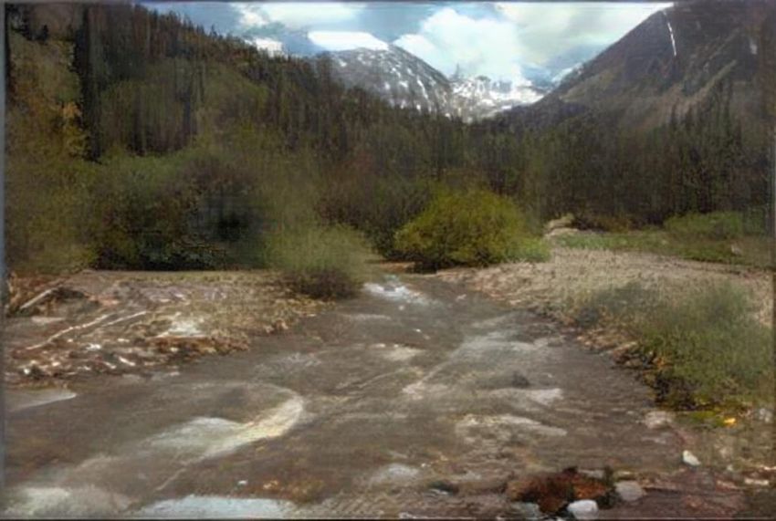
2         E. Agustsson, M. Tschannen, F. Mentzer, R. Timofte, and L. Van Gool

                                                                       m
                 w       ŵ                 x
                                                          w       ŵ
x            E       q        G                       E       q

                                       D                                   G
                                  x̂
s                                           s         F                             D
                                                                               x̂

(a) Global generative compression (GC)      (b) Selective generative compression (SC)

Fig. 2: Structure of the proposed compression networks. E is the encoder for the
image x and optionally the semantic label map s. q quantizes the latent code
w to ŵ. G is the generator, producing the decompressed image x̂, and D the
discriminator used for adversarial training. For SC, F extracts features from s
and the subsampled heatmap multiplies ẑ (pointwise) for spatial bit allocation.

These systems often outperform state-of-the-art engineered codecs such as BPG
[1], WebP [2], and JPEG2000 [3] on perceptual metrics [4–8]. Besides achiev-
ing higher compression rates on natural images, they can be easily adapted to
specific target domains such as stereo or medical images, and promise efficient
processing and indexing directly from compressed representations [9]. However,
for bitrates below 0.1 bits per pixel (bpp) these algorithms still incur severe
quality reductions. More generally, as the bitrate tends to zero, preserving the
full image content becomes impossible and common distortion measures such as
peak signal-to-noise ratio (PSNR) or multi-scale structural similarity (MS-SSIM)
[10] become meaningless as they favor exact preservation of local (high-entropy)
structure over preserving texture. To further advance deep image compression
it is therefore of great importance to develop new training objectives beyond
PSNR and MS-SSIM. A promising candidate towards this goal are adversarial
losses [11] which were shown recently to capture global semantic information
and local texture, yielding powerful generators that produce visually appealing
high resolution images from semantic label maps [12, 13].
    In this paper, we propose and study a generative adversarial network (GAN)-
based framework for extreme image compression, targeting bitrates below 0.1
bpp. We present a principled GAN formulation for deep image compression that
allows for different degrees of content generation. In contrast to prior works on
deep image compression which applied adversarial losses to image patches for
artifact suppression [6, 14] and generation of texture details [15] or representation
learning for thumbnail images [16], our generator/decoder operates on the full-
resolution image and is trained with a multi-scale discriminator [13].
    We study two modes of operation (corresponding to unconditional and con-
ditional GANs [11, 17]), namely

    – global generative compression (GC), preserving the overall image content
      while generating structure of different scales such as leaves of a tree or win-
      dows in the facade of buildings, and
    – selective generative compression (SC), completely generating parts of the
      image from a semantic label map while preserving user-defined regions with
      a high degree of detail.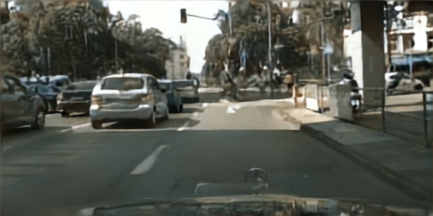
Generative Adversarial Networks for Extreme Learned Image Compression        3

    A typical use case for GC are bandwidth constrained scenarios, where one
wants to preserve the full image as much as possible, while falling back to syn-
thesized content instead of blocky/blurry blobs for regions where there are not
sufficient bits to store the original pixels. SC could be applied in a video call
scenario where one wants to fully preserve people in the video stream, but a
visually pleasing synthesized background serves our purpose as well as the true
background. In the GC operation mode the image is transformed into a bit-
stream and encoded using arithmetic coding. SC requires a semantic/instance
label map of the original image which can be obtained using off-the-shelf seman-
tic/instance segmentation networks, e.g., PSPNet [18] and Mask R-CNN [19],
and which is stored as a vector graphic. This amounts to a small, image dimen-
sion independent overhead in terms of coding cost. On the other hand, the size
of the compressed image is reduced proportionally to the area which is generated
from the semantic label map, typically leading to a significant overall reduction
in storage cost.
    For GC, a comprehensive user study shows that our compression system
yields visually considerably more appealing results than BPG [1] (the current
state-of-the-art engineered compression algorithm) and the recently proposed
autoencoder-based deep compression (AEDC) system [8]. In particular, for the
street scene images from the Cityscapes data set, users prefer the images pro-
duced by our method over BPG even when BPG uses more than double the
bits. To the best of our knowledge, these are the first results showing that a
deep compression method outperforms BPG in a user study. In the SC operation
mode, our system seamlessly combines preserved image content with synthesized
content, even for regions that cross multiple object boundaries. By partially gen-
erating image content we achieve bitrate reductions of over 50% without notably
degrading image quality. In both cases, the semantic information as measured
by the mean intersection over union (mIoU) between the semantic label maps of
the original and reconstructed image is significantly better preserved as for the
two baselines [1, 8].

2     Related work

Deep image compression has recently emerged as an active area of research. The
most popular DNN architectures for this task are to date auto-encoders [4, 5,
20, 21, 9] and recurrent neural networks (RNNs) [22, 23]. These DNNs transform
the input image into a bit-stream, which is in turn losslessly compressed using
entropy coding methods such as Huffman coding or arithmetic coding. To re-
duce coding rates, many deep compression systems rely on context models to
capture the distribution of the bit stream [5, 23, 21, 6, 8]. Common loss functions
to measure the distortion between the original and decompressed images are the
mean-squared error (MSE) [4, 5, 20, 21, 7, 9], or perceptual metrics such as MS-
SSIM [23, 6–8]. Some authors rely on advanced techniques including multi-scale
image decompositions [6], progressive encoding/decoding strategies [22, 23], and
generalized divisive normalization (GDN) layers [5, 24].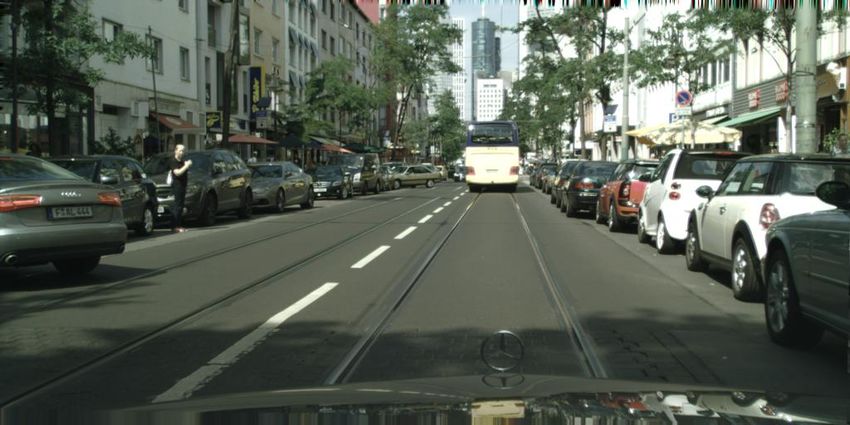
4      E. Agustsson, M. Tschannen, F. Mentzer, R. Timofte, and L. Van Gool

    Generative adversarial networks (GANs) [11] have emerged as a popular tech-
nique for learning generative models for intractable distributions in an unsuper-
vised manner. Despite stability issues [25–28], they were shown to be capable
of generating more realistic and sharper images than prior approaches such as
Variational Autoencoders [29]. While initially struggling with generating high
resolution images [30, 25], they were steadily improved, now reaching resolu-
tions of 1024 × 1024px [31, 32] for some datasets. Another direction that has
shown great progress are conditional GANs [11, 17], obtaining impressive results
for image-to-image translation [12, 13, 33, 34] on various datasets (e.g. maps to
satellite images), reaching resolutions as high as 1024 × 2048px [13].
    Arguably the most closely related work to ours is [6], which uses an adver-
sarial loss term to train a deep compression system. However, this loss term is
applied to small image patches and its purpose is to suppress artifacts rather
than to generate image content. Furthermore, it uses a non-standard GAN for-
mulation that does not (to the best of our knowledge) have an interpretation in
terms of divergences between probability distributions, as in [11, 35]. [16] uses
a GAN framework to learn a generative model over thumbnail images, which
is then used as a decoder for thumbnail image compression. Other works use
adversarial training for compression artifact removal (for engineered codecs) [14]
and single image super-resolution [15]. Finally, related to our SC mode, spatially
allocating bitrate based on saliency of image content has a long history in the
context of engineered compression algorithms, see e.g. [36–38].

3     Background
3.1   Generative Adversarial Networks
Given a data set X , Generative Adversarial Networks (GANs) can learn to ap-
proximate its (unknown) distribution px through a generator G(z) that tries to
map samples z from a fixed prior distribution pz to the distribution px .
   The generator G is trained in parallel with a discriminator D by search-
ing (using stochastic gradient descent (SGD)) for a saddle point of a mini-max
objective
                    min max       E[f (D(x))] + E[g(D(G(z)))],                (1)
                     G    D

where G and D are DNNs and f and g are scalar functions. The original paper
[11] uses the “Vanilla GAN” objective with f (y) = log(y) and g(y) = log(1 − y).
This corresponds to G minimizing the KL Divergence between the distribution
of x and G(z). The KL Divergence is a member of a more generic family of
f -divergences, and Nowozin et al.[35] show that for suitable choices of f and
g, all such divergences can be minimized with (1). In particular, if one uses
f (y) = (y − 1)2 and g(y) = y 2 , one obtains the Least-Squares GAN [28] (which
corresponds to the Pearson χ2 divergence), which we adopt in this paper. We
refer to the divergence minimized over G as
                 LGAN := max E[f (D(x))] + E[g(D(G(z)))].                     (2)
                              D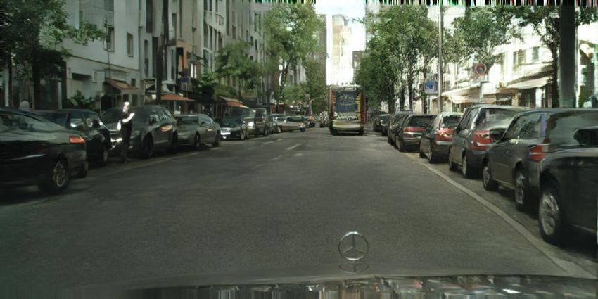
Generative Adversarial Networks for Extreme Learned Image Compression         5

3.2    Conditional Generative Adverarial Networks
For conditional GANs (cGANs) [11, 17], each data point x is associated with
additional information s, where (x, s) have an unknown joint distribution px,s .
We now assume that s is given and that we want to use the GAN to model
the conditional distribution px|s . In this case, both the generator G(z, s) and
discriminator D(z, s) have access to the side information s, leading to the diver-
gence

               LcGAN := max E[f (D(x, s))] + E[g(D(G(z, s), s))],               (3)
                          D

3.3    Deep Image Compression
To compress an image x ∈ X , we follow the formulation of [20, 8] where one
learns an encoder E, a decoder G, and a finite quantizer q. The encoder E
maps the image to a latent feature map w, whose values are then quantized
to L levels {c1 , · · · , cL } ⊂ R to obtain a representation ŵ = q(E(x)) that can
be encoded to a bitstream. The decoder then tries to the recover the image by
forming a reconstruction x̂ = G(ŵ). To be able to backpropagate through the
non-differentiable q, one can use a differentiable relaxation of q, as in [8].
    The average number of bits needed to encode ŵ is measured by the entropy
H(ŵ), which can be modeled with a prior [20] or a conditional probability model
[8]. The trade-off between reconstruction quality and bitrate to be optimized is
then
                                   E[d(x, x̂)] + βH(ŵ).                         (4)
where d is a loss that measures how perceptually similar x̂ is to x.
    Given a differentiable model of the entropy H(ŵ), the weight β controls
the bitrate of the model (high β pushes the bitrate down). However, since the
number of dimensions dim(ŵ) and the number of levels L are finite, the entropy
is bounded by (see, e.g., [39])

                              H(ŵ) ≤ dim(ŵ) log2 (L).                         (5)

It is therefore also valid to set β = 0 and control the maximum bitrate through
the bound (5) (i.e., adjusting L or dim(ŵ) through the architecture of E). While
potentially leading to suboptimal bitrates, this avoids to model the entropy
explicitly as a loss term.

4     GANs for extreme image compression
4.1    Global generative Compression
Our proposed GANs for extreme image compression can be viewed as a combi-
nation of (conditional) GANs and learned compression. With an encoder E and
quantizer q, we encode the image x to a compressed representation ŵ = q(E(x)).
This representation is optionally concatenated with noise v drawn from a fixed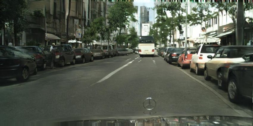
6      E. Agustsson, M. Tschannen, F. Mentzer, R. Timofte, and L. Van Gool

prior pv , to form the latent vector z. The decoder/generator G then tries to gen-
erate an image x̂ = G(z) that is consistent with the image distribution px while
also recovering the specific encoded image x to a certain degree (see Fig. 2 (a)).
Using z = [ŵ, v], this can be expressed by our saddle-point objective for (non-
conditional) generative compression,
      min max    E[f (D(x))] + E[g(D(G(z))] + λE[d(x, G(z))] + βH(ŵ),        (6)
      E,G   D

where λ > 0 balances the distortion term against the GAN loss and entropy
terms. Using this formulation, we need to encode a real image, ŵ = E(x), to
be able to sample from pŵ . However, this is not a limitation as our goal is to
compress real images and not to generate completely new ones.
   Since the last two terms of (6) do not depend on the discriminator D, they
do not affect its optimization directly. xThis means that the discriminator still
computes the same f divergence LGAN as in (2), so we can write (6) as
                    min   LGAN + λE[d(x, G(z))] + βH(ŵ).                     (7)
                    E,G

    We note that equation (6) has completely different dynamics than a normal
GAN, because the latent space z contains ŵ, which stores information about
a real image x. A crucial ingredient is the bitrate limitation on H(ŵ). If we
allow ŵ to contain arbitrarily many bits by setting β = 0 and letting L and
dim(ŵ) be large enough, E and G could learn to near-losslessly recover x from
G(z) = G(q(E(x))), such that the distortion term would vanish. In this case,
the divergence between px and pG(z) would also vanish and the GAN loss would
have no effect.
    By constraining the entropy of ŵ, E and G will never be able to make d
fully vanish. In this case, E, G need to balance the GAN objective LGAN and
the distortion term λE[d(x, G(z))], which leads to G(z) on one hand looking
“realistic”, and on the other hand preserving the original image. For example, if
there is a tree for which E cannot afford to store the exact texture (and make
d small) G can synthesize it to satisfy LGAN , instead of showing a blurry green
blob.
    In the extreme case where the bitrate becomes zero (i.e., H(ŵ) → 0, e.g.,
by setting β = ∞ or dim(ŵ) = 0), ŵ becomes deterministic. In this setting, z
is random and independent of x (through the v component) and the objective
reduces to a standard GAN plus the distortion term, which acts as a regularizer.
    We refer to the setting in (6) as global generative compression (GC), since
E, G balance reconstruction and generation automatically over the entire image.
    As for the conditional GANs in Sec. 3.2, we can easily extend the global
generative compression of the previous section to a conditional case. Here, we
also consider this setting, where the additional information s for an image x is
a semantic label map of the scene (see dashed lines in Fig. 2 (a)), with a small
difference: Instead of feeding the semantics to G, we give them to the encoder
E as an input. This avoids separately encoding the information s, since it is
contained in the representation ŵ. As for the conditional GAN, D also receives
the semantics s as an input.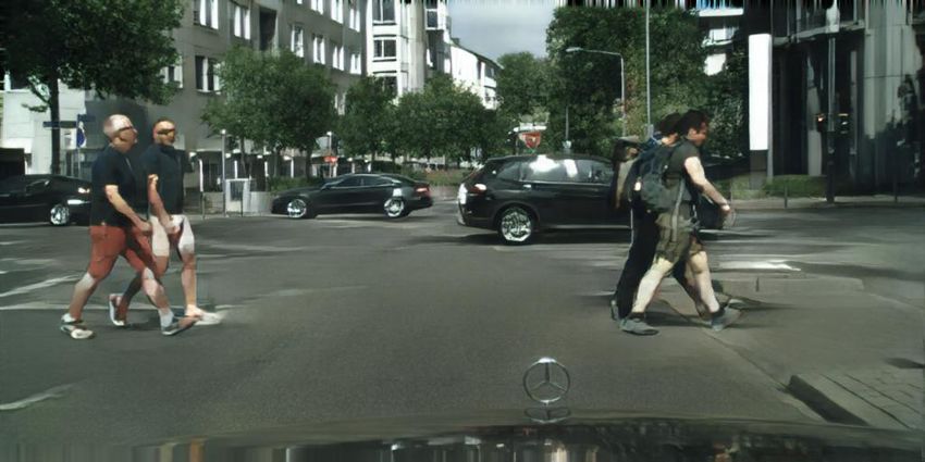
Generative Adversarial Networks for Extreme Learned Image Compression       7

4.2    Selective Generative Compression
For the global generative compression and its conditional variant described in the
previous section, E, G automatically navigate the trade-off between generation
and preservation over the entire image, without any guidance. Here, we consider
a different setting, where we guide the network in terms of which regions should
be preserved and which regions should be synthesized. We refer to this setting
as selective generative compression (SC) and give an overview in Fig. 2 (b).
    For simplicity, we consider a binary setting, where we construct a single-
channel binary heatmap m of the same spatial dimensions as ŵ. Regions of
zeros correspond to regions that should be fully synthesized, whereas regions of
ones correspond to regions that should be preserved. However, since our task
is compression, we constrain the fully synthesized regions to have the same se-
mantics s as the original image x. We assume the semantics s are separately
stored, and thus feed them through a feature extractor F before feeding them to
the generator G. To guide the network with the semantics, we mask the (pixel-
wise) distortion d, such that it is only computed over the region to be preserved.
Additionally, we zero out the latent feature ŵ in the regions that should be syn-
thesized. Provided that the heatmap m is also stored, we then only encode the
entries of ŵ corresponding to the preserved regions, greatly reducing the bitrate
needed to store it.
    At bitrates where ŵ is normally much larger than the storage cost for s and
m (about 2kB per image when encoded as a vector graphic), this approach can
give large bitrate savings.

5     Experiments
5.1    Network Architecture
The architecture for our encoder E and generator G is based on the global
generator network proposed in [13], which in turn is based on the architecture
of [40].
    For the GC, the encoder E convolutionally processes the image x and option-
ally the label map s, with spatial dimension W × H, into a feature map of size
W      H
 16 × 16 × 960 (with 6 layers, of which four have 2-strided convolutions), which
is then projected down to C channels (where C ∈ {2, 4, 8, 16} is much smaller
than 960). This results in a feature map w of dimension W         H
                                                             16 × 16 × C, which
is quantized over L centers to obtain the discrete ŵ. The generator G projects
ŵ up to 960 channels, processes these with 9 residual units [41] at dimension
W     H
 16 × 16 ×960, and then mirrors E by convolutionally processing the features back
to spatial dimensions W × H (with transposed convolutions instead of strided
ones).
    Similar to E, the feature extractor F for SC processes the semantic map
s down to the spatial dimension of ŵ, which is then concatenated to ŵ for
generation. In this case, we consider slightly higher bitrates and downscale by
8× instead of 16× in the encoder E, such that dim(ŵ) = W            H
                                                                8 × 8 × C. The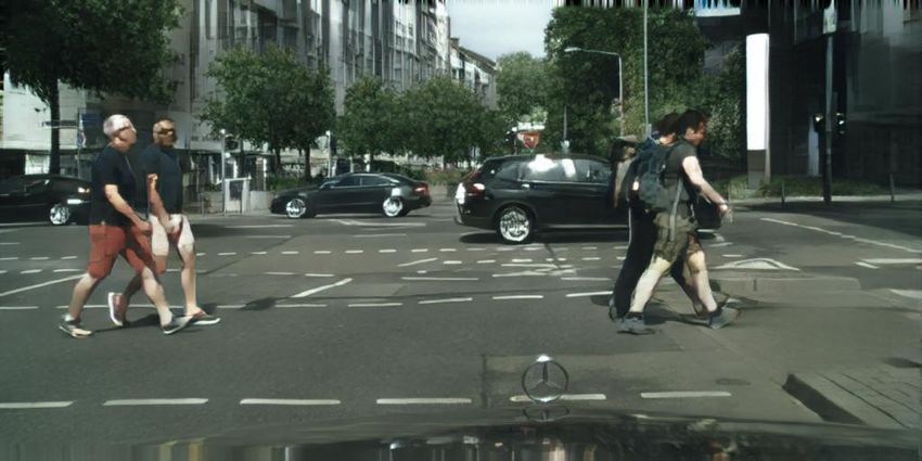
8      E. Agustsson, M. Tschannen, F. Mentzer, R. Timofte, and L. Van Gool

generator then first processes ŵ down to W    H
                                          16 × 16 × 960 and then proceeds as for
GC.
    For both GC and SC, we use the multi-scale architecture of [13] for the
discriminator D, which measures the divergence between px and pG(z) both
locally and globally.

5.2   Losses and Hyperparameters
For the entropy term βH(ŵ), we adopt the simplified approach described in
Sec. 3.3, where we set β = 0, use L = 5 centers C = {−2, 1, 0, 1, 2}, and control
the bitrate through the upper bound H(ŵ) ≤ dim(ŵ) log2 (L). For example, for
GC, with C = 2 channels, we obtain
                               ×H
          H(ŵ)   log2 (5) · W
                             16·16 · 2
                =                      = 0.0181 bits per pixel (bpp).
          W ×H          W ×H
We note that this is an upper bound; the actual entropy of H(ŵ) is generally
smaller, since the learned distribution will neither be uniform nor i.i.d, which
would be required for the bound to hold with equality. By using a histogram as
in [20] or a context model as in [8], we could reduce this bitrate either in a post
processing step, or jointly during training as in the respective works.
    For the distortion term we adopt d(x, x̂) = MSE with coefficient λ = 10.
Furthermore, we adopt the feature matching and VGG perceptual losses, LFM
and LVGG , as proposed in [13] with the same weights, which improved the quality
for images synthesized from semantic label maps. These losses can be viewed as
a part of d(x, x̂). However, we do not mask them in SC, since they also help to
stabilize the GAN in this operation mode (as in [13]).

5.3   Evaluation
Data sets: We train the proposed method on two popular data sets that come
with hand-annotated semantic label maps, namely Cityscapes [42] and ADE20k
[43]. Both of these data sets were previously used with GANs [12, 33], hence
we know that GANs can model their distribution—at least to a certain extent.
Cityscapes contains 2975 training and 500 validation images of dimension 2048×
1024px, which we resampled to 1024 × 512px for our experiments. The training
and validation images are annotated with 34 and 19 classes, respectively. From
the ADE20k data set we use the SceneParse150 subset with 20 210 training and
2000 validation images of a wide variety of sizes (200×200px to 975×975px), each
annotated with 150 classes. During training, the ADE20k images are rescaled
such that the width is 512px.

Generalization to Kodak: The Kodak image compression dataset [44] has a long
tradition in the image compression literature and is still the most frequently
used dataset for comparisons.
   While we do not have training data nor semantic labels available for the
Kodak dataset, our GC models can also be trained without semantic maps and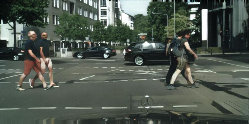
Generative Adversarial Networks for Extreme Learned Image Compression      9

thus do not need such labels at test time. Thus we can assess how well our
models generalize to Kodak by training GC without semantics on ADE20k (i.e.,
non-conditional) and then testing on Kodak. The only adjustment we made
when using our models was to slightly blur the images (σ = 1.0) to avoid large
gradients in the images which are not present in the training data (due to re-
sizing with anti-aliasing). We did not observe any improvement for BPG when
using blur, so we used BPG with standard settings.

Baselines: We compare our method to the HEVC-based image compression al-
gorithm BPG [1] (in the default 4:2:2 chroma format) and to the AEDC net-
work [8]. BPG is the current state-of-the-art engineered image compression codec
and outperforms other recent codecs such as JPEG2000 and WebP on different
data sets in terms of MS-SSIM (see, e.g., [6]). We train the AEDC network (with
bottleneck depth C = 4) on Cityscapes exactly following the procedure in [8]
except that we use early stopping to prevent overfitting (note that Cityscapes is
much smaller than the ImageNet dataset used in [8]). The so-obtained model has
a bitrate of 0.07 bpp and obtains a slightly better MS-SSIM than BPG at the
same bpp on the validation set. As an additional baseline, we train our partial
synthesis with an MSE loss only (all other training parameters are maintained,
see Sec. 5.4).

Quantitative evaluation: Quality measures such as PSNR and MS-SSIM com-
monly used to assess the quality of compression systems become meaningless at
very low bitrates as they penalize changes in local structure rather than preser-
vation of the global content (this also becomes apparent through our baseline
trained for MSE, see Sec. 5.5). We therefore measure the capacity of our method
to preserve the image semantics as proxy for the image quality and compare
it with the baselines. Specifically, we use PSPNet [45] and compute the mean
intersection-over-union (IoU) between the label map obtained for the decom-
pressed validation images and the ground truth label map. A similar approach
was followed by image translation works [12, 13] to asses image quality of gener-
ated images.

User study: To quantitatively evaluate the perceptual quality of our GC networks
in comparison with BPG and AEDC we conduct a user study using the Amazon
Mechanical Turk (AMT) platform1 . For Cityscapes we consider 3 settings for
our method using C = 2, 4, 8 which correspond to 0.018, 0.036, and 0.072 bpp,
respectively, and perform one-to-one comparisons of the images produced by our
method to those of AEDC at 0.07 bpp and BPG at 5 operating points in the range
[0.039, 0.1] bpp. A slightly different setup is used for ADE20k: We only consider
the 0.036 and 0.072 operating points, and employ the GC network trained with
semantic label map for the latter operating point. To test the generalization to
the Kodak dataset [44], we used the model trained on ADE20k for 0.036bpp.
    For each pairing of methods on Cityscapes and ADE20K, we compare the
decompressed images obtained for a set of 20 randomly picked validation images,
1
    https://www.mturk.com/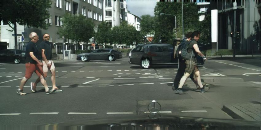
10     E. Agustsson, M. Tschannen, F. Mentzer, R. Timofte, and L. Van Gool

having as reference the downscaled 1024 × 512px images. For each pairing on
Kodak, we used all 24 images of the dataset. 9 randomly selected users were
asked to select the best decompression result for each test image and pairing of
methods.

Visual comparisons: Finally, we perform extensive visual comparisons of all our
methods and the baselines (see supplementary material for more examples).

5.4   Training
We employ the ADAM optimizer [46] with a learning rate of 0.0002 and set the
mini-batch size to 1. Our networks are trained for 50 epochs on Cityscapes and
for 20 epochs on ADE20k, aside from the network tested on Kodak which was
trained for 50 epochs on ADE20k.
    For SC we consider two different training modes: Random instance (RI)
which randomly selects 25% of the instances in the semantic label map and
preserves these, and random box (RB) which picks an image location uniformly
at random and preserves a box of dimensions randomly selected from the interval
[200, 400] and [150, 300] for Cityscapes and ADE20k, respectively. While the RI
mode is appropriate for most use cases, the RB can create more challenging
situations for the generator as it needs to integrate the preserved box seamlessly
into the generated content. Additionally, we add a MSE loss term between the
input image and the reconstructed image, acting on the masked region only, for
training SC networks.

5.5   Results
Global generative compression: Fig. 5 (left) shows the mean IoU on the Cityscapes
validation set as a function of bpp for our GC networks with C = 2, 4, 8, along
with the values obtained for the baselines. Additionally, we plot mean IoU for
our network trained with an MSE loss, and the networks obtained when feeding
semantic label maps to E and D during training. It can be seen that at a given
target bpp, our networks outperform BPG and AEDC as well as our network
trained for MSE by a large margin. Furthermore, feeding the semantic labels to
the encoder and discriminator increases the mean validation IoU.
    In Tables 1 and 2 we report the percentages of preference of the image pro-
duced by the proposed method over the image produced by the other compression
method for Cityscapes and ADE20k, respectively. For each method vs. method
comparison 180 human opinions were collected. For both data sets, the per-
ceptual quality of our results is better than that of the baseline approaches at
comparable bpp. For Cityscapes, at 0.036 bpp our method is picked by the users
over BPG in 81.87% of the cases, while at 0.072 bpp our method is preferred
over BPG and AEDC in 70.18% and 84.21% of the cases, respectively.
    In Figs. 1, 3, and 4 we present example validation images from Cityscapes
and ADE20k, respectively, produced by our GC networks at different bpp along
with the images obtained from the baseline algorithms at the same bpp. The GC
Generative Adversarial Networks for Extreme Learned Image Compression 11
Ours (0.072bpp) BPG (0.074bpp) AEDC (0.074bpp)
Fig. 3: Visual example of images produced by our GC network with C = 8 along
with the corresponding results for BPG and AEDC.
Ours (0.036bpp) BPG (0.092bpp) Ours (0.072bpp) BPG (0.082bpp)
Fig. 4: Visual examples of images produced by our GC networks (left: C = 4;
right: C = 8) along with the corresponding results for BPG.
produces images with finer structure than BPG, which suffers from smoothed
patches and blocking artifacts. AEDC and our network trained for MSE both
produce blurry images.
Generalization to Kodak: We show the results for an example Kodak image in
Figure 6, obtained with a model trained on ADE20K for GC (without seman-
tics) using C = 4 channels (0.036bpp). While there is some color shift noticeable
(which could be accounted for by reducing the domain mismatch and/or increas-
ing the weight of the perceptual loss), we see that our method can realistically
synthesize details where BPG fails.
The user study results in Table 3 shows that our method is preferred over
BPG, even when BPG uses an 80% larger bitrate of 0.065bpp compared to our
method at 0.036bpp.
Selective generative compression: We plot the mean IoU for the Cityscapes val-
idation set for our SC networks and the baselines in Fig. 5 (right) as a function
of bpp. Again, our networks obtain a higher mean IoU than the baselines at the
same bpp, for both the RI and RB training modes. The mean IoU is almost
constant as a function of bpp.12 E. Agustsson, M. Tschannen, F. Mentzer, R. Timofte, and L. Van Gool
Preference of BPG [1] AEDC [8]
our results [%] vs. 0.039 bpp 0.056 bpp 0.072 bpp 0.079 bpp 0.1 bpp 0.069 bpp
C = 2, 0.018 bpp 76.02 52.05 45.03 38.01 29.24 71.93
our
C = 4, 0.036 bpp 81.87 67.25 59.65 50.88 35.67 80.12
C = 8, 0.072 bpp 83.63 74.27 70.18 67.84 50.88 84.21
Table 1: User study quantitative preferences results [%] on Cityscapes. For each
pairing of methods we report the percentage of cases in which the image produced
by our GC method was preferred by human subjects over the result of the other
compression method. For comparable bpp our method is clearly the preferred
method. On average, BPG is only perceptually better than ours when a bitrate
more than twice as large is used.
Preference of BPG [1]
our results [%] vs. 0.054 bpp 0.064 bpp 0.072 bpp 0.082 bpp 0.1 bpp
C = 4, 0.036 bpp 66.67 52.63 36.26 / /
our
C = 8, 0.072 bpp, w. sem. 80.12 73.68 57.31 52.63 41.52
Table 2: User study quantitative preferences results [%] on ADE20k. For com-
parable bpp our method is clearly preferred.
Preference of BPG [1]
our results [%] vs. 0.038 bpp 0.060 bpp 0.065 bpp 0.072 bpp
our C = 4, 0.036 bpp 87.10 57.60 54.84 47.00
Table 3: User study quantitative preferences results [%] on Kodak. Our method is
preferred over BPG at 0.065bpp, which corresponds to a 45% bitrate reduction.
mIoU vs. bpp (GC) mIoU vs. bpp (SC)
50% 50%
Ours (semantics)
Ours
Ours (MSE)
40% 40%
BPG
AEDC
30% 30%
20% 20%
Ours (instance)
Ours (box)
Ours (MSE)
10% 10% BPG
AEDC
pix2pixHD
0.00 0.02 0.04 0.06 0.08 0.10 0.12 0.00 0.04 0.08 0.12 0.16 0.20
Fig. 5: Left: Mean IoU as a function of bpp on the Cityscapes validation set for
our GC networks, optionally trained with semantic label maps at G and D (se-
mantics) and with MSE loss only (MSE). Right: Mean IoU for our SC networks
trained in the RI (instance) and RB (box) training modes. The pix2pixHD base-
line [13] was trained from scratch for 50 epochs, using the same downsampled
1024 × 512px training images as for our method.Generative Adversarial Networks for Extreme Learned Image Compression 13
Kodak Image 13 Ours (0.036bpp)
BPG (0.073bpp) JPEG2000 (0.037bpp)
WebP (0.078bpp) JPEG (0.248bpp)
Fig. 6: Original Kodak Image 13 along with the decompressed version used in
the user study (Ours), obtained using our GC network with C = 4. We also
show decompressed BPG, JPEG, JPEG2000, and WebP versions of the image.
If a codec was not able to produce an output as low as 0.036bpp, we chose the
lowest possible bitrate for that codec.
Fig. 7 and 8 show example Cityscapes validation images produced by the
SC network trained in the RI mode with C = 8 and C = 4, respectively, where
different semantic classes are preserved. While classes such as trees and street
look more realistic than less structured classes such as buildings or cars, most
configurations of masks yield visually pleasing results, while leading to large bpp14 E. Agustsson, M. Tschannen, F. Mentzer, R. Timofte, and L. Van Gool
road (0.146 bpp, -55%) car (0.227 bpp, -15%) everything (0.035 bpp, -89%)
people (0.219 bpp, -33%) building (0.199 bpp, -39%) no synth. (0.326 bpp, -0%)
Fig. 7: Synthesizing different classes using our SC network with C = 8. In each
image except for no synthesis, we additionally synthesize the classes vegetation,
sky, sidewalk, ego vehicle, wall. The heatmaps in the lower left corners show the
synthesized parts in gray. We show the bpp of each image as well as the relative
savings due to the selective generation.
base (0.062 bpp) +buildings (0.038 bpp) BPG (0.043 bpp)
Fig. 8: Example image obtained by our SC network (C = 4) synthesizing road,
vegetation, sky, sidewalk, ego vehicle, wall for “base” on the left and additionally
building in the center. Right shows BPG at the lowest supported bpp.
Original 0.103bpp 0.103bpp
Fig. 9: Example image obtained by our SC network (C = 8) preserving a box
and synthesizing the rest of the image.
reductions compared to the network preserving the entire image. Notably, the
GC network can generate an entire image from the semantic label map only.
In Fig. 9 we present an example Cityscapes validation image produced by an
SC network (with C = 8) trained in the RB mode, with a rectangular area pre-
served. Our network seamlessly integrates the preserved region into the generated
part of the image. Fig. 10 shows example images from the ADE20k validation
set produced by SC networks (with C = 8) for both the RB and RI training
mode.Generative Adversarial Networks for Extreme Learned Image Compression 15
Fig. 10: Example ADE20k validation images produced by our SC network with
(C = 8) preserving randomly selected instances (left, network trained with RI)
or box-shaped regions (right, network trained with RB).
6 Discussion
The quantitative evaluation of the semantic preservation capacity (Fig. 5) indi-
cates that both the GC and the SC networks better preserve semantics than the
baselines at the same bpp when evaluated with PSPNet. This has to be taken
with a grain of salt, however, in the cases where our networks are provided with
the semantic label maps. It is not surprising that these networks outperform
BPG and AEDC, which were not designed or trained specifically to preserve
semantic information. Note though that our GC network only drops slightly in
mIoU when trained without semantics (Fig. 5 left), still having much higher
semantic preservation capacity than BPG and AEDC.
Qualitatively, our GC networks preserve more and sharper structure than the
baseline methods, for both the Cityscapes and ADE20k images. For both data
sets, the user study shows that at a given target bpp humans on average prefer
the pictures produced by our GC networks over BPG. For Cityscapes, where we
trained an AEDC model, our images are on average also preferred over AEDC.
The Cityscapes images obtained by our GC networks with C = 2 (0.018bpp)
and C = 4 (0.036 bpp) were even preferred over BPG at 0.056 and BPG at
0.079 bpp, respectively, showing that our method outperforms BPG even when
BPG uses more than twice as many bits. For ADE20k, the results produced by
our GC networks were preferred on average by a considerable margin over BPG,
although the preference is less pronounced than for Cityscapes.
Furthermore, we found that our model trained on ADE20K (With minor
adjustments) can also generalize well to the Kodak dataset, being preferred over
BPG for C = 4 (0.036bpp) even when BPG uses 80% more bits.
We note that while prior works [6, 8, 7] have outperformed BPG in terms
of MS-SSIM[10], they have not demonstrated improved visual quality over BPG
(which is optimized for PSNR). In particular, [7, 8] show a visual comparison but
do not claim improved visual quality over BPG, whereas [6] does not compare
with BPG visually. To the best of our knowledge, this is the first time that a
deep compression method is shown to outperform BPG in a user study—and
that with a large margin.16 E. Agustsson, M. Tschannen, F. Mentzer, R. Timofte, and L. Van Gool
In the SC operation mode, our networks manage to seamlessly merge pre-
served and generated image content both when preserving object instances or
boxes crossing object boundaries. Further, our networks lead to reductions in
bpp of 50% and more compared to the same networks without synthesis, while
leaving the visual quality essentially unimpaired, when objects with repetitive
structure are synthesized (such as trees, streets, and sky). In some cases, the
visual quality is even better than that of BPG at the same bitrate. The visual
quality of more complex synthesized objects (e.g., buildings, people) is worse.
However, this is a limitation of current GAN technology rather than our ap-
proach. As the visual quality of GANs improves further, SC networks will as
well. Moreover, our SC networks are based on simple entropy coding without
context model and it is not surprising that they do not outperform BPG in chal-
lenging scenarios (in the case where no synthesis is performed, see Fig. 7). Indeed,
BPG relies on advanced techniques including context modeling. We note that
this is mainly an engineering problem; our networks could be extended using,
e.g., the context model from [8].
Finally, the semantic label map, which requires 0.036 bpp on average for
the downscaled 1024 × 512px Cityscapes images, represents a relatively large
overhead compared to the storage cost of the preserved image parts. This cost
vanishes as the image size increases, since the semantic mask can be stored as an
image dimension-independent vector graphic. Unfortunately, we could not train
our models (nor the model of [13]) for images larger than 1024 × 512px as this
requires a GPU with 24GB of memory (see [13]). We tried training on crops to
reduce the memory usage, but this led to poor results—which could be explained
by the fact that the discriminator then does not have a global view of the image
anymore.
7 Conclusion
We have proposed a GAN formulation of learned compression that significantly
outperforms prior works for low bitrates, both in terms of mIoU and human opin-
ion. Furthermore, our networks can seamlessly combine preserved with generated
image content, producing realistic looking images when synthesizing content with
regular structure.
Promising directions for future work are to develop a mechanism to control
spatial allocation of bits for GC, and to combine SC with saliency information.
Furthermore, it would be interesting to incorporate a context model into our
method, for example the one from [8], and to adapt the architecture so that it
scales to even larger images.Generative Adversarial Networks for Extreme Learned Image Compression 17
References
1. Bellard, F.: BPG Image format. https://bellard.org/bpg/
2. : WebP Image format. https://developers.google.com/speed/webp/
3. Taubman, D.S., Marcellin, M.W.: JPEG 2000: Image Compression Fundamentals,
Standards and Practice. Kluwer Academic Publishers, Norwell, MA, USA (2001)
4. Theis, L., Shi, W., Cunningham, A., Huszar, F.: Lossy image compression with
compressive autoencoders. In: International Conference on Learning Representa-
tions (ICLR). (2017)
5. Ballé, J., Laparra, V., Simoncelli, E.P.: End-to-end optimized image compression.
arXiv preprint arXiv:1611.01704 (2016)
6. Rippel, O., Bourdev, L.: Real-time adaptive image compression. In: Proceedings
of the 34th International Conference on Machine Learning. Volume 70 of Pro-
ceedings of Machine Learning Research., International Convention Centre, Sydney,
Australia, PMLR (06–11 Aug 2017) 2922–2930
7. Ballé, J., Minnen, D., Singh, S., Hwang, S.J., Johnston, N.: Variational image
compression with a scale hyperprior. In: International Conference on Learning
Representations (ICLR). (2018)
8. Mentzer, F., Agustsson, E., Tschannen, M., Timofte, R., Van Gool, L.: Conditional
probability models for deep image compression. In: IEEE Conference on Computer
Vision and Pattern Recognition (CVPR). (2018)
9. Torfason, R., Mentzer, F., Ágústsson, E., Tschannen, M., Timofte, R., Gool, L.V.:
Towards image understanding from deep compression without decoding. In: Inter-
national Conference on Learning Representations (ICLR). (2018)
10. Wang, Z., Simoncelli, E.P., Bovik, A.C.: Multiscale structural similarity for image
quality assessment. In: Asilomar Conference on Signals, Systems Computers, 2003.
Volume 2. (Nov 2003) 1398–1402 Vol.2
11. Goodfellow, I., Pouget-Abadie, J., Mirza, M., Xu, B., Warde-Farley, D., Ozair, S.,
Courville, A., Bengio, Y.: Generative adversarial nets. In: Advances in neural
information processing systems. (2014) 2672–2680
12. Isola, P., Zhu, J.Y., Zhou, T., Efros, A.A.: Image-to-image translation with condi-
tional adversarial networks. In: Proceedings of the IEEE Conference on Computer
Vision and Pattern Recognition. (2017) 1125–1134
13. Wang, T.C., Liu, M.Y., Zhu, J.Y., Tao, A., Kautz, J., Catanzaro, B.: High-
resolution image synthesis and semantic manipulation with conditional gans. In:
IEEE Conference on Computer Vision and Pattern Recognition (CVPR). (2018)
14. Galteri, L., Seidenari, L., Bertini, M., Del Bimbo, A.: Deep generative adversarial
compression artifact removal. In: Proceedings of the IEEE Conference on Computer
Vision and Pattern Recognition. (2017) 4826–4835
15. Ledig, C., Theis, L., Huszar, F., Caballero, J., Cunningham, A., Acosta, A., Aitken,
A., Tejani, A., Totz, J., Wang, Z., et al.: Photo-realistic single image super-
resolution using a generative adversarial network. In: Proceedings of the IEEE
Conference on Computer Vision and Pattern Recognition. (2017) 4681–4690
16. Santurkar, S., Budden, D., Shavit, N.: Generative compression. arXiv preprint
arXiv:1703.01467 (2017)
17. Mirza, M., Osindero, S.: Conditional generative adversarial nets. arXiv preprint
arXiv:1411.1784 (2014)
18. Zhao, H., Shi, J., Qi, X., Wang, X., Jia, J.: Pyramid scene parsing network. In:
Proceedings of IEEE Conference on Computer Vision and Pattern Recognition
(CVPR). (2017)18 E. Agustsson, M. Tschannen, F. Mentzer, R. Timofte, and L. Van Gool
19. He, K., Gkioxari, G., Dollár, P., Girshick, R.: Mask r-cnn. In: Computer Vision
(ICCV), 2017 IEEE International Conference on, IEEE (2017) 2980–2988
20. Agustsson, E., Mentzer, F., Tschannen, M., Cavigelli, L., Timofte, R., Benini, L.,
Van Gool, L.: Soft-to-hard vector quantization for end-to-end learning compressible
representations. arXiv preprint arXiv:1704.00648 (2017)
21. Li, M., Zuo, W., Gu, S., Zhao, D., Zhang, D.: Learning convolutional networks for
content-weighted image compression. arXiv preprint arXiv:1703.10553 (2017)
22. Toderici, G., O’Malley, S.M., Hwang, S.J., Vincent, D., Minnen, D., Baluja, S.,
Covell, M., Sukthankar, R.: Variable rate image compression with recurrent neural
networks. arXiv preprint arXiv:1511.06085 (2015)
23. Toderici, G., Vincent, D., Johnston, N., Hwang, S.J., Minnen, D., Shor, J., Covell,
M.: Full resolution image compression with recurrent neural networks. arXiv
preprint arXiv:1608.05148 (2016)
24. Ballé, J., Laparra, V., Simoncelli, E.P.: End-to-end optimization of nonlinear trans-
form codes for perceptual quality. arXiv preprint arXiv:1607.05006 (2016)
25. Salimans, T., Goodfellow, I., Zaremba, W., Cheung, V., Radford, A., Chen, X.:
Improved techniques for training gans. In: Advances in Neural Information Pro-
cessing Systems. (2016) 2234–2242
26. Arjovsky, M., Bottou, L.: Towards principled methods for training generative
adversarial networks. arXiv preprint arXiv:1701.04862 (2017)
27. Arjovsky, M., Chintala, S., Bottou, L.: Wasserstein gan. arXiv preprint
arXiv:1701.07875 (2017)
28. Mao, X., Li, Q., Xie, H., Lau, R.Y., Wang, Z., Smolley, S.P.: Least squares gener-
ative adversarial networks. In: 2017 IEEE International Conference on Computer
Vision (ICCV), IEEE (2017) 2813–2821
29. Kingma, D.P., Welling, M.: Auto-encoding variational bayes. arXiv preprint
arXiv:1312.6114 (2013)
30. Radford, A., Metz, L., Chintala, S.: Unsupervised representation learn-
ing with deep convolutional generative adversarial networks. arXiv preprint
arXiv:1511.06434 (2015)
31. Zhang, H., Xu, T., Li, H., Zhang, S., Huang, X., Wang, X., Metaxas, D.: Stack-
gan: Text to photo-realistic image synthesis with stacked generative adversarial
networks. In: IEEE Int. Conf. Comput. Vision (ICCV). (2017) 5907–5915
32. Karras, T., Aila, T., Laine, S., Lehtinen, J.: Progressive growing of gans for im-
proved quality, stability, and variation. In: International Conference on Learning
Representations (ICLR). (2017)
33. Zhu, J.Y., Park, T., Isola, P., Efros, A.A.: Unpaired image-to-image translation us-
ing cycle-consistent adversarial networks. In: Proceedings of the IEEE Conference
on Computer Vision and Pattern Recognition. (2017) 2223–2232
34. Liu, M.Y., Breuel, T., Kautz, J.: Unsupervised image-to-image translation net-
works. In: Advances in Neural Information Processing Systems. (2017) 700–708
35. Nowozin, S., Cseke, B., Tomioka, R.: f-gan: Training generative neural samplers
using variational divergence minimization. In: Advances in Neural Information
Processing Systems. (2016) 271–279
36. Stella, X.Y., Lisin, D.A.: Image compression based on visual saliency at individual
scales. In: International Symposium on Visual Computing, Springer (2009) 157–
166
37. Guo, C., Zhang, L.: A novel multiresolution spatiotemporal saliency detection
model and its applications in image and video compression. IEEE transactions on
image processing 19(1) (2010) 185–198Generative Adversarial Networks for Extreme Learned Image Compression 19
38. Gupta, R., Khanna, M.T., Chaudhury, S.: Visual saliency guided video compression
algorithm. Signal Processing: Image Communication 28(9) (2013) 1006–1022
39. Cover, T.M., Thomas, J.A.: Elements of information theory. John Wiley & Sons
(2012)
40. Johnson, J., Alahi, A., Fei-Fei, L.: Perceptual losses for real-time style transfer
and super-resolution. In: European Conference on Computer Vision. (2016)
41. He, K., Zhang, X., Ren, S., Sun, J.: Deep residual learning for image recognition.
In: IEEE Conference on Computer Vision and Pattern Recognition (CVPR). (June
2016)
42. Cordts, M., Omran, M., Ramos, S., Rehfeld, T., Enzweiler, M., Benenson, R.,
Franke, U., Roth, S., Schiele, B.: The Cityscapes Dataset for Semantic Urban
Scene Understanding. ArXiv e-prints (April 2016)
43. Zhou, B., Zhao, H., Puig, X., Fidler, S., Barriuso, A., Torralba, A.: Scene parsing
through ade20k dataset. In: Proceedings of the IEEE Conference on Computer
Vision and Pattern Recognition. (2017)
44. : Kodak PhotoCD dataset. http://r0k.us/graphics/kodak/
45. Zhao, H., Shi, J., Qi, X., Wang, X., Jia, J.: Pyramid Scene Parsing Network. ArXiv
e-prints (December 2016)
46. Kingma, D.P., Ba, J.: Adam: A method for stochastic optimization. CoRR
abs/1412.6980 (2014)20 E. Agustsson, M. Tschannen, F. Mentzer, R. Timofte, and L. Van Gool
Generative Adversarial Networks for Extreme Learned
Image Compression: Supplementary Material
A Compression details
Recall that we use the upper bound Eq. (5) to control the entropy of the bit-
stream when training our networks. To verify that this upper bound is tight, we
computed the actual bitrate in bpp for our GC network with C = 4 using an
arithmetic coding implementation. We find that using a uniform prior, it matches
the theoretical bound up to the third significant digit. If we use a non-uniform
per-image probability model, we obtain a bitrate reduction of 1.7%.
We compress the semantic label map for SC by quantizing the coordinates
in the vector graphic to the image grid and encoding coordinates relative to
preceding coordinates when traversing object boundaries (rather than relative to
the image frame). The so-obtained bitstream is then compressed using arithmetic
coding.
To ensure fair comparison, we do not count header sizes for any of the baseline
methods throughout.
B Architecture details
We adopt the notation from [13] to describe our encoder and generator/decoder
architectures and additionally use q to denote the quantization layer (see Sec.
3.3 for details). The output of q is encoded and stored.
– Encoder GC: c7s1-60,d120,d240,d480,d960,c3s1-C,q
– Encoders SC:
• Semantic label map encoder: c7s1-60,d120,d240,d480,d960
• Image encoder: c7s1-60,d120,d240,d480,c3s1-C,q,c3s1-480,d960
The outputs of the semantic label map encoder and the image encoder are
concatenated and fed to the generator/decoder.
– Generator/decoder: c3s1-960,R960,R960,R960,R960,R960,R960,R960,
R960,R960,u480,u240,u120,u60,c7s1-3
C Visuals
In Sec. C.1 and C.2 we present further visual example images from Cityscapes
and ADE20k, respectively, obtained for SC when preserving randomly selected
semantic classes or boxes (see Sec. 5.3 for details on the experiments). The
Cityscapes, ADE20k, and Kodak images used in the user study along with the
corresponding BPG images are shown in Sec. C.3, C.4, and C.52 .
2
https://data.vision.ee.ethz.ch/aeirikur/extremecompression/files/suppC5.pdfGenerative Adversarial Networks for Extreme Learned Image Compression 21
C.1 Selective Compression (Cityscapes)
road (0.077 bpp) car (0.108 bpp) everything (0.041 bpp)
people (0.120 bpp) building (0.110 bpp) no synth (0.186 bpp)
road (0.092 bpp) car (0.134 bpp) everything (0.034 bpp)
people (0.147 bpp) building (0.119 bpp) no synth (0.179 bpp)
Fig. 11: Synthesizing different classes for two different images from Cityscapes,
using our SC network with C = 4. In each image except for no synthesis, we
additionally synthesize the classes vegetation, sky, sidewalk, ego vehicle, wall.
Fig. 12: Example images obtained by our SC network (C = 8) preserving a box
and synthesizing the rest of the image, on Cityscapes.22 E. Agustsson, M. Tschannen, F. Mentzer, R. Timofte, and L. Van Gool C.2 Selective Compression (ADE20k) Fig. 13: Example ADE20k validation images obtained by our SC network (C = 8) preserving a box and synthesizing the remaining image area. The original images are shown for comparison.
Generative Adversarial Networks for Extreme Learned Image Compression   23

Fig. 14: Preserving randomly chosen semantic classes in ADE20k validation im-
ages and synthesizing the remaining image area using our SC network with
C = 8. The original images are shown for comparison.
24        E. Agustsson, M. Tschannen, F. Mentzer, R. Timofte, and L. Van Gool

C.3      Global Compression (Cityscapes)

     Ours (0.036bpp)    BPG (0.034bpp)      Ours (0.036bpp)     BPG (0.041bpp)

     Ours (0.036bpp)    BPG (0.043bpp)      Ours (0.036bpp)     BPG (0.033bpp)

     Ours (0.036bpp)    BPG (0.050bpp)      Ours (0.036bpp)     BPG (0.037bpp)

     Ours (0.036bpp)    BPG (0.037bpp)      Ours (0.036bpp)     BPG (0.035bpp)

     Ours (0.036bpp)    BPG (0.051bpp)      Ours (0.036bpp)     BPG (0.048bpp)
Fig. 15: Decompressed versions of the first 10 images used in the user study on
Cityscapes, obtained using our GC network with C = 4 and BPG.
Generative Adversarial Networks for Extreme Learned Image Compression 25 Ours (0.036bpp) BPG (0.036bpp) Ours (0.036bpp) BPG (0.034bpp) Ours (0.036bpp) BPG (0.038bpp) Ours (0.036bpp) BPG (0.037bpp) Ours (0.036bpp) BPG (0.038bpp) Ours (0.036bpp) BPG (0.033bpp) Ours (0.036bpp) BPG (0.037bpp) Ours (0.036bpp) BPG (0.036bpp) Ours (0.036bpp) BPG (0.036bpp) Ours (0.036bpp) BPG (0.037bpp) Fig. 16: Decompressed versions of images 11 − 20 used in the user study on Cityscapes, obtained using our GC network with C = 4 and BPG.
26       E. Agustsson, M. Tschannen, F. Mentzer, R. Timofte, and L. Van Gool

C.4     Global Compression (ADE20k)

 Ours (0.036bpp)   BPG (0.036bpp)   Ours (0.036bpp)   BPG (0.055bpp)   Ours (0.036bpp)   BPG (0.050bpp)

 Ours (0.036bpp)   BPG (0.059bpp)   Ours (0.036bpp)   BPG (0.085bpp)   Ours (0.036bpp)   BPG (0.037bpp)

 Ours (0.036bpp)   BPG (0.082bpp)   Ours (0.036bpp)   BPG (0.038bpp)   Ours (0.036bpp)   BPG (0.034bpp)

 Ours (0.036bpp)   BPG (0.075bpp)   Ours (0.036bpp)   BPG (0.061bpp)   Ours (0.036bpp)   BPG (0.079bpp)

Fig. 17: Decompressed versions of the first 12 images used in the user study on
ADE20k, obtained using our GC network with C = 4 and BPG.
Generative Adversarial Networks for Extreme Learned Image Compression            27

             Ours (0.036bpp)   BPG (0.054bpp)   Ours (0.036bpp)   BPG (0.037bpp)

             Ours (0.036bpp)   BPG (0.074bpp)   Ours (0.036bpp)   BPG (0.036bpp)

             Ours (0.036bpp)   BPG (0.065bpp)   Ours (0.036bpp)   BPG (0.037bpp)

             Ours (0.036bpp)   BPG (0.137bpp)   Ours (0.036bpp)   BPG (0.036bpp)

Fig. 18: Decompressed versions of images 12 − 20 used in the user study on
ADE20k, obtained using our GC network with C = 4 and BPG.
You can also read