Self-Supervised Deep Visual Odometry with Online Adaptation
←
→
Page content transcription
If your browser does not render page correctly, please read the page content below
Self-Supervised Deep Visual Odometry with Online Adaptation

                                               Shunkai Li    Xin Wang      Yingdian Cao      Fei Xue      Zike Yan    Hongbin Zha
                                                  Key Laboratory of Machine Perception (MOE), School of EECS, Peking University
                                                                     PKU-SenseTime Machine Vision Joint Lab
                                              {lishunkai, xinwang cis, yingdianc, feixue, zike.yan}@pku.edu.cn                                   zha@cis.pku.edu.cn
arXiv:2005.06136v1 [cs.CV] 13 May 2020

                                                                  Abstract

                                             Self-supervised VO methods have shown great success
                                         in jointly estimating camera pose and depth from videos.
                                         However, like most data-driven methods, existing VO net-
                                         works suffer from a notable decrease in performance when
                                         confronted with scenes different from the training data,
                                         which makes them unsuitable for practical applications. In
                                         this paper, we propose an online meta-learning algorithm to
                                         enable VO networks to continuously adapt to new environ-
                                         ments in a self-supervised manner. The proposed method
                                         utilizes convolutional long short-term memory (convLSTM)
                                         to aggregate rich spatial-temporal information in the past.
                                         The network is able to memorize and learn from its past
                                         experience for better estimation and fast adaptation to the
                                         current frame. When running VO in the open world, in order
                                         to deal with the changing environment, we propose an on-                 Figure 1. We demonstrate the domain shift problem for self-
                                         line feature alignment method by aligning feature distribu-              supervised VO. Previous methods fail to generalize when the
                                         tions at different time. Our VO network is able to seamlessly            test data are different from the training data. In contrast, our
                                         adapt to different environments. Extensive experiments on                method performs well when tested on changing environments,
                                         unseen outdoor scenes, virtual to real world and outdoor to              which demonstrates the advantage of fast online adaptation
                                         indoor environments demonstrate that our method consis-
                                         tently outperforms state-of-the-art self-supervised VO base-
                                                                                                                  from the training dataset [8, 37] (Fig. 1). When applied a
                                         lines considerably.
                                                                                                                  pre-trained VO network to the open world, the inability to
                                                                                                                  generalize itself to new scenes presents a serious problem
                                                                                                                  for its practical applications. This requires the VO network
                                         1. Introduction
                                                                                                                  to continuously adapt to the new environment.
                                            Simultaneous localization and mapping (SLAM) and vi-                      In contrast to fine-tuning a pre-trained network with
                                         sual odometry (VO) play a vital role for many real-world                 ground truth data on the target domain [37], it is unlikely
                                         applications, such as autonomous driving, robotics and                   to collect enough data in advance when running VO in the
                                         mixed reality. Classic SLAM/VO [13, 14, 17, 29] methods                  open world. This requires the network to adapt itself in real-
                                         perform well in regular scenes but fail in challenging condi-            time to changing environments. In this online learning set-
                                         tions (e.g. dynamic objects, occlusions, textureless regions)            ting, there is no explicit distinction between training and
                                         due to their reliance on low-level features. Since deep learn-           testing phases — we learn as we perform. This is much
                                         ing is able to extract high-level features and infer in an end-          different from conventional learning methods where a pre-
                                         to-end fashion, learning-based VO [22, 40, 41, 44] methods               trained model is fixed during inference.
                                         have been proposed in recent years to alleviate the limita-                  During online adaptation, the VO network can only learn
                                         tion of classic hand-engineered algorithms.                              from the current data instead of the entire training data with
                                            However, learning-based VO suffers from a notable de-                 batch training and multiple epoches [11]. The learning ob-
                                         crease in accuracy when confronted with scenes different                 jective is to find an optimal model that is well adapted to

                                                                                                           4321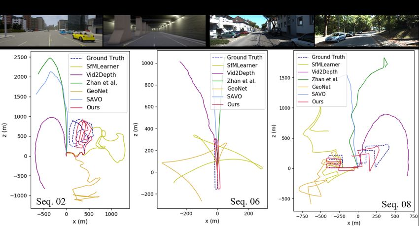
the current data. However, because of the limited temporal             and depth to learn by minimizing photometric loss. Yin et
perceptive field [26], the current optimal model may not be            al. [41] and Ranjan et al. [32] extend this idea to joint esti-
well suited for subsequent frames. This makes the optimal              mation of pose, depth and optical flow to handle non-rigid
parameters oscillate with time, leading to slow convergence            cases which are against static-scene assumption. These
during online adaptation [9, 11, 20].                                  methods focus on mimicking local structure from motion
    In order to address these issues, we propose an online             (SfM) with image pairs, but fail to exploit spatial-temporal
meta-learning scheme for self-supervised VO that achieves              correlations over long sequence. SAVO [22] formulates VO
online adaptation. The proposed method motivates the net-              as a sequential generative task and utilizes RNN to reduce
work to perform consistently well at different time by incor-          scale drift significantly. In this paper, we adopt the same
porating online adaptation process into the learning objec-            idea as SfMLearner [44] and SAVO [22].
tive. Besides, the past experience can be used to accelerate               Online adaptation Most machine learning models suf-
the adaptation to a new environment. Therefore, instead                fer from a significant reduce in performance when the test
of learning only from the current data, we employ convo-               data are different from the training set. An effective solution
lutional long short-term memory (convLSTM) to aggregate                to alleviate this domain shift issue is online learning [35],
rich spatial-temporal information in the video that enables            where data are processed sequentially and data distribution
the network to use past experience for better estimation and           changes continuously. Previous methods use online gra-
also adapt quickly to the current frame. In order to achieve           dient update [12] and probabilistic filtering [6]. Recently,
fast adaptation in changing environments, we propose a fea-            domain adaptation has been widely studied in computer vi-
ture alignment method to align non-stationary feature distri-          sion. Long et al. [23] propose Maximum Mean Discrepancy
butions at different time. The proposed network automati-              loss to reduce the domain shift. Several works [5, 33] utilize
cally adapts to changing environments without ground truth             Generative Adversarial Networks (GAN) to directly trans-
data collected in advance for external supervision. Our con-           fer images in the target domain to the source domain (e.g.
tributions can be summarized as follows:                               day to night or winter to summer). Inspired by [5, 7], we
                                                                       propose a feature alignment method for online adaptation.
  • We propose an online meta-learning algorithm for VO
                                                                           Meta-learning, or learning to learn, is a continued in-
    to continuously adapt to unseen environments in a self-
                                                                       terest in machine learning. It exploits inherent structures in
    supervised manner.
                                                                       data to learn more effective learning rules for fast domain
  • The VO network utilizes past experience incorporated               adaptation [27, 36]. A popular approach is to train a meta-
    by convLSTM to achieve better estimation and adapt                 learner that learns how to update the network [4, 15]. Finn
    quickly to the current frame.                                      et al. [15, 16] proposed Model Agnostic Meta-Learning
                                                                       (MAML) that constrains the learning rule for the model
  • We propose a feature alignment method to deal with                 and uses stochastic gradient descent to quickly adapt net-
    the changing data distributions in the open world.                 works to new tasks. This simple yet effective formulation
    Our VO network achieves 32 FPS on a Geforce 1080Ti                 has been widely used to adapt deep networks to unseen en-
GPU with online refinement, making it adapt in real-time               vironments [1, 2, 21, 30, 39]. Our proposed method is most
for practical applications. We evaluate our algorithm across           relevant to MAML, which extends it to the self-supervised,
different domains, including outdoor, indoor and synthetic             online learning setting.
environments, which consistently outperforms state-of-the-
art self-supervised VO baselines.                                      3. Problem setup
                                                                       3.1. Self-supervised VO
2. Related works
                                                                           Our self-supervised VO follows the similar idea of SfM-
   Learning-based VO has been widely studied in recent
                                                                       Learner [44] and SAVO [22] (shown in Fig. 2). The Depth-
years with the advent of deep learning and many meth-
                                                                       Net predicts depth D̂t of the current frame It . The PoseNet
ods with promising results have been proposed. Inspired
                                                                       takes stacked monocular images It−1 , It and D̂t−1 , D̂t to
by the framework of parallel tracking and mapping in clas-
                                                                       regress relative pose T̂tt−1 . Then view synthesis is applied
sic SLAM/VO, DeepTAM [43] utilizes two networks for
                                                                       to reconstruct Iˆt by differentiable image warping:
pose and depth estimation simultaneously. DeepVO [38]
uses recurrent neural network (RNN) to leverage sequential                            pt−1 ∼ K T̂tt−1 D̂t (pt )K −1 pt ,          (1)
correlations to estimate poses recurrently. However, these
methods require ground truth which is expensive or im-                 where pt−1 , pt are the homogeneous coordinates of a pixel
practical to obtain. To avoid the need of annotated data,              in It−1 and It , respectively. K denotes camera intrinsics.
self-supervised VO has been recently developed. SfM-                   The MaskNet predicts a per-pixel mask M̂t [44] according
Learner [44] utilizes the 3D geometric constraint of pose              to the warping residuals kIˆt − It k1 .

                                                                4322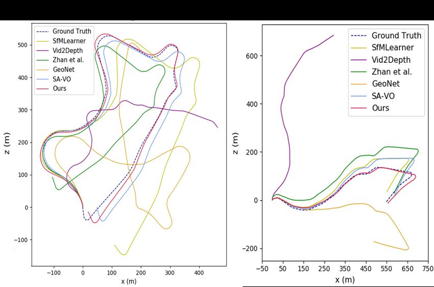
Figure 2. The framework of our method. The VO network estimates pose T̂tt−1 , depth D̂t , D̂t−1 and mask M̂t from image sequences
Di . At each iteration i, the network parameters θi are updated according to the loss L and performs inference for Di+1 at next time. The
network learns to find a set of weights θi∗ that perform well both for Di and Di+1 . During online learning, spatial-temporal information is
aggregated by convLSTM and feature alignment is adopted to align feature distributions F̂i , F̂i+1 at different time for fast adaptation

3.2. Online adaptation                                                      leads to slow convergence and may introduce negative bias
                                                                            in the learning procedure.
   As shown in Fig. 1, the performance of VO networks is
fundamentally limited by their generalization ability when
                                                                            4. Method
confronted with scenes different from the training data. The
reason is they are designed under a closed world assump-                        In order to address these issues, we propose to exploit
tion: the training data Dtrain and test data Dtest are i.i.d.               correlations of different time for fast online adaptation. Our
sampled from a common dataset with fixed distribution.                      framework is illustrated in Fig. 2. The VO network θi takes
However, when running a pre-trained VO network in the                       N consecutive frames in the sliding window Di to estimate
open world, images are continuously collected in changing                   pose and depth in a self-supervised manner (Sec. 3.1). Then
scenes. In this sense, the training and test data no longer                 it is updated according to the loss L and infers for frames
share similar visual appearances, and the data at the current               Di+1 at the next time. The network learns to find a set of
view may be different from previous views. This requires                    weights θi∗ to perform well both for Di and Di+1 (Sec. 4.1).
the network to online adapt to changing environments.                       During online learning, spatial-temporal information is in-
   Given a model θ pretrained on Dtrain , a naive approach                  corporated by convLSTM (Sec. 4.2) and feature alignment
for online learning is to update parameters θ by computing                  is adopted (Sec. 4.3) for fast adaptation.
loss L on the current data Di :
                                                                            4.1. Self-supervised online meta-learning
                 θi+1 = θi − α∇θi L(θi , Di ),                 (2)
                                                                               In contrast to L(θi , Di ), we extend the online learning
where θ0 = θ and α is the learning rate. Despite its sim-                   objective to L(θi+1 , Di+1 ), which can be written as:
plicity, this approach has several drawbacks. The tempo-
ral perceptive field of the learning objective L(θi , Di ) is 1,                        min L(θi − α∇θi L(θi , Di ), Di+1 ).            (3)
                                                                                         θi
which means it accounts only for the current input Di and
has no correlation with previous data. The optimal solu-                    Different from naive online learning, the temporal percep-
tion for current Di is likely to be unsuitable for subsequent               tive field of Eq. 3 becomes 2. It optimizes the performance
inputs. Therefore, the gradients ∇θi L(θi , Di ) at different               on Di+1 after adapting to the task on Di . The insight is
iterations are stochastic without consistency [9, 26]. This                 instead of minimizing the training error L(θi , Di ) on the

                                                                     4323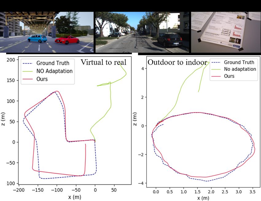
current iteration i, we try to minimize the test error on the              slow convergence. In contrast, the second term enforces
next iteration. Our formulation directly incorporates online               consistent gradient directions by aligning gradient for Di+1
adaptation into the learning objective, which motivates the                with previous information, indicating that we are training
network to learn θi at i to perform better at next time i + 1.             the network θi at i to perform consistently well for both i
   Our objective of learning to adapt is similar in spirit to              and i + 1. This meta-learning scheme alleviates stochastic
that of Model Agnostic Meta Learning (MAML) [15]:                          gradient problem in online learning. Eq. 6 describes the dy-
               X                                                           namics of sequential learning in non-stationary scenes. The
          min       L(θ − α∇θ L(θ, Dτtrain ), Dτval ),     (4)             network learns to adjust at current state by L(θi , Di ) to bet-
            θ
                  τ ∈T                                                     ter perform at next time. Consequently, the learned θ is less
which aims to minimize the evaluation (adaptation) error on                sensitive to the non-stationary data distributions of sequen-
the validation set instead of minimizing the training error on             tial inputs, enabling fast adaptation to unseen environments.
the training set. τ denotes tasks sampled from the task set
                                                                           4.2. Spatial-temporal aggregation
T . More details of MAML can be found in [15].
    As a nested optimization problem, our objective function                  As stated in Sec. 1, online learning suffers from slow
is optimized via a two-stage gradient descent. At each itera-              convergence due to the inherent limitation of temporal per-
tion i, we take N consecutive frames in the sliding window                 ceptive field. In order to make online updating more effec-
as a mini-dataset Di (shown within the blue area in Fig. 2):               tive, we let the network perform current estimation based on
                                                                           previous information. Besides, predicting pose from only
                Di = {It , It−1 , It−2 , . . . , It−N +1 }.   (5)          image pairs is prone to error accumulation. This trajec-
                                                                           tory drift problem can be mitigated by exploiting spatial-
In the inner loop of Eq. 3, we evaluate the performance of
                                                                           temporal correlations over long sequence [22, 40].
VO in Di by self-supervised loss L and update parameters
                                                                              In this paper, we use convolutional LSTM (convLSTM)
θi according to Eq. 2. Then, in the outer loop, we evaluate
                                                                           to achieve fast adaptation and reduce accumulated error. As
the performance of the updated model θi+1 on subsequent
                                                                           shown in Fig. 3, we embed recurrent units into the encoder
frames Di+1 . We mimic this continuous adaptation process
                                                                           of DepthNet and PoseNet to allow the convolutional net-
on both training and online test phases. During training, we
                                                                           work to leverage not only spatial but also temporal informa-
minimize the sum of losses by Eq. 3 across all sequences
                                                                           tion for depth and pose estimation. The length N of convL-
in the training dataset, which motivates the network to learn
                                                                           STM is the number of frames in Di . ConvLSTM acts as the
base weights θ that enables fast online adaptation.
                                                                           memory of the network. As new frames are processed, the
    In order to provide more intuition on what it learns and
                                                                           network is able to memorize and learn from its past experi-
the reason for fast adaptation, we take Taylor expansion on
                                                                           ence, so as to update parameters to quickly adapt to unseen
our training objective:
                                                                           environments. This approach not only enforces correlations
min L(θi − α∇θi L(θi , Di ), Di+1 )                                        among different time steps, but also learns the temporally
  θi
                                                                           dynamic nature of the moving camera from video inputs.
 ≈ min L(θi , Di+1 ) − α∇θi L(θi , Di ) · ∇θi L(θi , Di+1 )
       θi

   + Hθi · [α∇θi L(θi , Di )]2 + . . .
 ≈ min L(θi , Di+1 ) − α h∇θi L(θi , Di ), ∇θi L(θi , Di+1 )i ,
       θi
                                                           (6)
where Hθi denotes Hessian matrix and h·, ·i denotes inner
product. Since most neural networks use ReLU activations,
the networks are locally linear, thus the second order deriva-
tive equals 0 in most cases [28]. Therefore, Hθt ≈ 0 and
higher order terms are also omitted.
   As shown in Eq. 6, the network learns to minimize the
prediction error L(θi , Di+1 ) with θi while maximizing the
similarity between the gradients at Di and Di+1 . Since the
camera is continuously moving, the scenes Di , Di+1 may
vary from different time. Naive online learning treats dif-
ferent scenes independently by fitting only the current scene
but ignores the way to perform VO in different scenes are                  Figure 3. Network architecture of DepthNet, PoseNet and
similar. As gradient indicates the direction to update the                 MaskNet in self-supervised VO framework. The height of each
network, this leads to inconsistent gradients at i, i + 1 and              block represents the size of its feature maps

                                                                    4324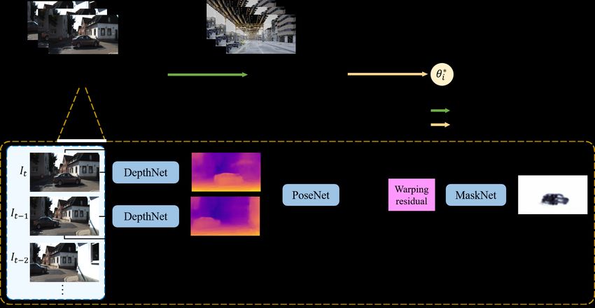
4.3. Feature alignment                                                    4.4. Loss functions
    One basic assumption of conventional machine learning                    Our self-supervised loss L is the same as most previous
is that the training and test data are independently and iden-            methods. It consists of:
tically (i.i.d.) drawn from the same distribution. However,                  Appearance loss We measure the reconstructed image Iˆ
this assumption does not hold when running VO in the open                 by photometric loss and structural similarity metric (SSIM):
world, since the test data (target domain) are usually dif-
                                                                                                    1 X
ferent from the training data (source domain). Besides, as                                              M̂ kIˆ − Ik1
                                                                             La = λm Lm (M̂ ) + (1 − αs )
the camera is continuously moving in the changing envi-                                            N
                                                                                                ˆ y), I(x, y))
                                                                                   1 X 1 − SSIM(I(x,                                (11)
ronment, the captured scenes Di also vary in time. As high-                      +       αs                     .
lighted in [7, 25], aligning feature distributions of two do-                      N x,y          2
mains will improve performance in domain adaptation.
    Inspired by [7], we extend this domain adaptation                     The regularization term Lm (M̂ ) prevents the learned mask
method to the online learning setting by aligning feature dis-            M̂ converges to a trivial solution [44]. The filter size of
tributions in different time. When training on the source do-             SSIM is set 5×5 and αs is set 0.85.
main, we collect the statistics of features fj ∈ {f1 , ..., fn }             Depth regularization We introduce an edge-aware loss
in a feature map tensor by Layer Normalization (LN) [3]:                  to enforce discontinuity and local smoothness in depth:
                    Fs = (µs , σs2 ),                                                     1 X
                 n                   n                                             Lr =         k∇x D̂(x, y)ke−k∇x I(x,y)k +
              1X          2     1X                                                        N x,y                                     (12)
         µs =       fj , σs =          (fj − µs )2 ,        (7)
              n j=1             n j=1                                                                      −k∇y I(x,y)k
                                                                                          k∇y D̂(x, y)ke                  .
                     n =H × W × C,
                                                                             Thus the self-supervised loss L is:
where H, W, C are the height, width and channels of each
feature map. When adapted to the target domain, we initial-                                   L = λa La + λr Lr .                   (13)
ize feature statistics at i = 0:
                                                                          5. Experiments
                          F0 = Fs .                        (8)
                                                                          5.1. Implementation details
Then at each iteration i, feature statistics F̂i = (µ̂i , σˆi2 )
are computed by Eq. 7. Given previous statistics Fi−1 =                       The architecture of our network is shown in Fig. 3. The
         2
(µi−1 , σi−1 ), feature distribution at i is aligned by:                  DepthNet uses a U-shaped architecture similar to [44]. The
                                                                          PoseNet is splited into 2 parts followed by fully-connected
                 µi = (1 − β)µi−1 + β µ̂i ,
                                                            (9)           layers to regress Euler angles and translations of 6-DoF
                 σi2 = (1 − β)σi−1
                               2
                                   + β σ̂i2 ,                             pose, respectively. The length of convLSTM N is set 9.
where β is a hyperparameter. After feature alignment, the                 Layer Normalization and ReLUs are adopted in each layer
features fj ∈ {f1 , ..., fn } are normalized to [3]:                      except for the output layers. Detailed network architecture
                                                                          can be found in the supplementary materials.
                            fj − µi
                    fˆj = γ p 2      + δ,                  (10)               Our model is implemented by PyTorch [31] on a single
                              σi +                                       NVIDIA GTX 1080Ti GPU. All sub-networks are jointly
where  is a small constant for numerical stability. γ and δ              trained in a self-supervised manner. Images are resized to
are the learnable scale and shift in normalization layers [3].            128×416 during both training and online adaptation. The
    The insight of this approach is to enforce correlation                Adam [19] optimizer with β1 = 0.9, β2 = 0.99 is used
of non-stationary feature distributions in changing environ-              and the weight decay is set 4 × 10⁻⁴ . Weighting factors
ments. Learning algorithms perform well when feature dis-                 λm , λa , λr are set 0.01, 1 and 0.5, respectively. The feature
tribution of the test data is the same as the training data.              alignment parameter β is set 0.5. The batch size is 4 for
When changed to a new environment, despite the extracted                  training and 1 for online adaptation. The learning objective
features are different, we deem that feature distributions of             (Eq. 3) is used for both training and online adaptation. We
two domains should be the same (Eq. 8). Despite the view                  pre-train the network for 20,000 iterations. The learning
is changing when running VO in an open world, Di and                      rate α of the inner loop and outer loop are both initialized
Di+1 are observed continuously in time, thus their feature                to 10−4 and reduced by half for every 5,000 iterations.
distributions should be similar (Eq. 9). This feature normal-
                                                                          5.2. Outdoor KITTI
ization and alignment approach acts as regularization that
simplifies the learning process, which makes the learned                     First, we test our method on KITTI odometry [18]
weights θ consistent for non-stationary environments.                     dataset. It contains 11 driving scenes with ground truth

                                                                   4325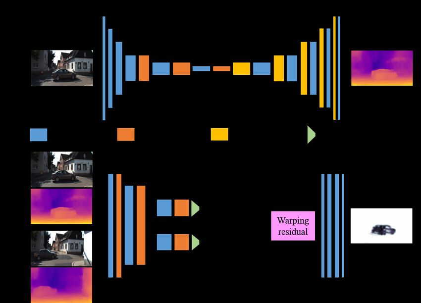
Method SfMLearner GeoNet Vid2Depth SAVO Ours
FPS 24 21 37 17 32
Table 2. Running speed of different VO methods.
5.3. Synthetic to real
Synthetic datasets (e.g. virtual KITTI, Synthia and Carla)
have been widely used for research since they provide
ground truth labels and controllable environment settings.
However, there’s a large gap between the synthetic and real-
world data. In order to test the domain adaptation ability, we
use Carla simulator [10] to collect synthetic images under
different weather conditions in the virtual city for training,
Figure 4. Trajectories of different methods on KITTI dataset. Our and use KITTI 00-10 for online testing.
method shows a better odometry estimation due to online updating It can be seen from Fig. 1, 5 and Table 3 that previous
methods all failed when shifted to real-world environments.
This is probably because the features of virtual scenes are
Method Seq. 09 Seq. 10 much different from the real world despite they are both col-
terr rerr terr rerr lected in the driving scenario. In contrast, our method sig-
SfMLearner [44] 11.15 3.72 5.98 3.40 nificantly outperforms previous arts, which is able to bridge
Vid2Depth [24] 44.52 12.11 21.45 12.50 the domain gap and quickly adapt to the real-world data.
Zhan et al. [42] 11.89 3.62 12.82 3.40
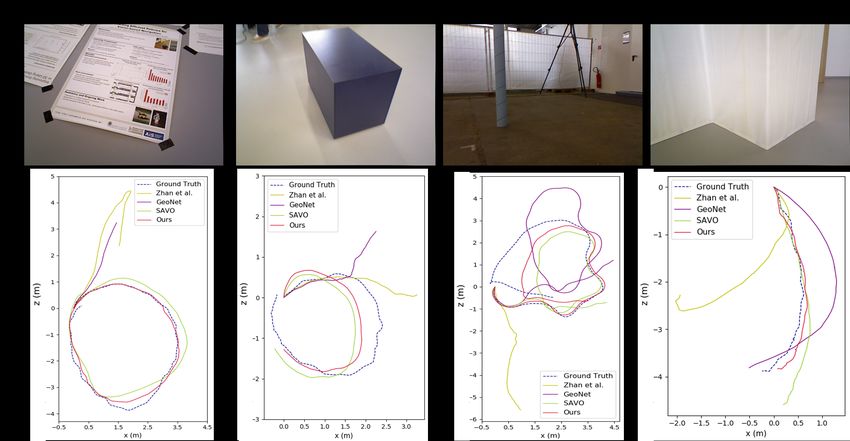
GeoNet [41] 23.94 9.81 20.73 9.10 5.4. Outdoor KITTI to indoor TUM
SAVO [22] 9.52 3.64 6.45 2.41
Ours 5.89 3.34 4.79 0.83 In order to further evaluate the adaptability of our
method, we test various baselines on TUM-RGBD [34]
Table 1. Quantitative comparison of visual odometry results on dataset. KITTI is captured by moving cars with planar mo-
KITTI dataset. terr : average translational root mean square error tion, high quality images and sufficient disparity. Instead,
(RMSE) drift (%); rerr : average rotational RMSE drift (◦ /100m) TUM dataset is collected by handheld cameras in indoor
scenes with much more complicated motion patterns, which
is significantly different from KITTI. It includes various
challenging conditions (Fig. 6) such as dynamic objects,
poses. We follow the same train/test split as [22, 41, 44]
non-texture scenes, abrupt motions and large occlusions.
using sequences 00-08 for training and 09-10 for online test.
We pretrain these methods on KITTI 00-08 and test on
Instead of calculating absolute trajectory error (ATE) on TUM dataset. Despite the ground truth depth is available,
image pairs in previous methods, we recover full trajecto- we only use monocular RGB images during test. It can be
ries and compute translation error terr by KITTI evaluation seen (Table 4 and Fig. 6) that our method consistently out-
toolkit, rotation error rerr . We compare our method with performs all the other baselines. Despite the large domain
several state-of-the-art self-supervised VO baselines: SfM- shift and significant difference in motion patterns (i.e. large,
Learner [44], GeoNet [41], Zhan et al. [42], Vid2Depth [24] planar motion vs small motion in 3 axes), our method can
and SAVO [22]. As stated in [24], a scaling factor is used to still recover trajectories well. On the contrary, GeoNet [41]
align trajectories with ground truth to solve the scale ambi- and Zhan et al. [42] tend to fail. Despite SAVO [22] uti-
guity problem in monocular VO. The estimated trajectories lizes LSTM to alleviate accumulated error to some extent,
of sequences 09-10 are plotted in Fig. 4 and quantitative our method performs better due to online adaptation.
evaluations are shown in Table 1. Our method outperforms
all the other baselines by a clear margin, the accumulated 5.5. Ablation studies
error is reduced by online adapation.
In order to demonstrate the effectiveness of each compo-
The comparison of the running speed with other VO nent, we present ablation studies on various versions of our
methods can be found in Table 2. Since we are studying the method on KITTI dataset (shown in Table 5).
online learning problem, the running time includes forward First, we evaluate the backbone of our method (the first
propagation, loss computing, back propagation and network row) which includes convLSTM and feature alignment but
updating. Our method achieves real-time online adaptation no meta-learning process during training and online test. It
and outperforms state-of-the-art baselines considerably. can be seen from Table 1 and Table 5 that, even without
4326Figure 5. Trajectories of different methods pretrained on Carla and test on KITTI dataset. Our method significantly outperforms all the
other baselines when changed from virtual to the real-world data
SfMLearner [44] Vid2Depth [24] Zhan et al. [42] GeoNet [41] SAVO [22] Ours
Seq frames terr rerr terr rerr terr rerr terr rerr terr rerr terr rerr
00 4541 61.55 27.13 61.69 28.41 63.30 28.24 44.08 14.89 60.10 28.43 14.21 5.93
01 1101 83.91 10.36 48.44 10.30 35.68 9.78 43.21 8.42 64.68 9.91 21.36 4.62
02 4661 71.48 27.80 70.56 25.72 84.63 24.67 73.59 12.53 69.15 24.78 16.21 2.60
03 801 49.51 36.81 41.92 27.31 50.05 16.44 43.36 14.56 66.34 16.45 18.41 0.89
04 271 23.80 10.52 39.34 3.42 12.08 1.56 17.91 9.95 25.28 1.84 9.08 4.41
05 2761 87.72 30.71 63.62 30.71 89.03 29.66 32.47 13.12 59.90 29.67 24.82 6.33
06 1101 59.53 12.70 84.33 32.75 93.66 30.91 40.28 16.68 63.18 31.04 9.77 3.58
07 1101 51.77 18.94 74.62 48.89 99.69 49.08 37.13 17.20 63.04 49.25 12.85 2.30
08 4701 86.51 28.13 70.20 28.14 87.57 28.13 33.41 11.45 62.45 27.11 27.10 7.81
09 1591 58.18 20.03 69.20 26.18 83.48 25.07 51.97 13.02 67.06 25.76 15.21 5.28
10 1201 45.33 16.91 49.10 23.96 53.70 22.93 46.63 13.80 58.52 23.02 25.63 7.69
Table 3. Quantitative comparisons of different methods pretraining on synthetic data in Carla simulator and testing on KITTI
Sequence Structure Texture Abrupt motion Zhan et al. [42] GeoNet [41] SAVO [22] Ours
fr2/desk X X - 0.361 0.287 0.269 0.214
fr2/pioneer 360 X X X 0.306 0.410 0.383 0.218
fr2/pioneer slam X X X 0.309 0.301 0.338 0.190
fr2/360 kidnap X X X 0.367 0.325 0.311 0.298
fr3/cabinet X - - 0.316 0.282 0.281 0.272
fr3/long off hou valid X X - 0.327 0.316 0.297 0.237
fr3/nstr tex near loop - X - 0.340 0.277 0.440 0.255
fr3/str ntex far X - - 0.235 0.258 0.216 0.177
fr3/str ntex near X - - 0.217 0.198 0.204 0.128
Table 4. Quantitative evaluation of different methods pretraining on KITTI and testing on TUM-RGBD dataset. We evaluate relative pose
error (RPE) which is presented as translational RMSE in [m/s]
4327Figure 6. Raw images (top) and trajectories (bottom) recovered by different methods on TUM-RGBD dataset
Seq. 09 Seq. 10 alignment during online adaptation. One possible explaina-
Online Pretrain LSTM FA terr rerr terr rerr tion is convLSTM incorporates spatial-temporal correla-
- Standard X X 10.93 3.91 11.65 4.11 tions and past experience over long sequence. It associates
Naive Standard X X 10.22 5.33 8.24 3.22 different states recurrently, making the gradient computa-
Meta Meta - - 9.25 4.20 7.58 3.13 tion graph more intensively connected during back propa-
Meta Meta X - 6.36 3.84 5.37 1.41 gation. Meanwhile, convLSTM correlates the VO network
Meta Meta - X 7.52 4.12 5.98 2.72
at different time, enforcing to learn a set of weights θ that
Meta Meta X X 5.89 3.34 4.79 0.83
are consistent in the dynamic environment.
Table 5. Quantitative comparison of ablation study on KITTI
Besides, we study how the size of sliding window N is
dataset for various versions of our method. FA: feature alignment influencing the VO performance. The change of N has no
much impact on the running speed (30-32 FPS), but as N
increases, the adaptation gets faster and better. When N is
meta-learning and online adaptation, our network backbone greater than 15, the adaptation speed and accuracy becomes
still outperforms most pervious methods. The results in- lower. Therefore, we set N = 15 as the best choice.
dicate that convLSTM is able to reduce accumulated error
and feature alignment improves the performance when con- 6. Conclusions
fronted with unseen environments. In this paper, we propose an online meta-learning
Then we compare the efficiency of naive online learning scheme for self-supervised VO to achieve fast online adap-
(the second row) and meta-learning (the last row). It can be tation in the open world. We use convLSTM to aggregate
seen that, although naive online learning is able to reduce spatial-temporal information in the past, enabling the net-
estimation error to some extent, it converges much slower work to use past experience for better estimation and fast
than the meta-learning scheme, indicating that it takes much adaptation to the current frame. Besides, we put forward a
longer time to adapt the network to the new environment. feature alignment method to deal with changing feature dis-
Finally, we study the effect of convLSTM and feature tributions in the unconstrained open world setting. Our net-
alignment during meta-learning (last four rows). Compared work dynamically evolves in time to continuously adapt to
with baseline meta-learning scheme, convLSTM and fea- changing environments on-the-fly. Extensive experiments
ture alignment give the VO performance a further boost. on outdoor, virtual and indoor datasets demonstrate that our
Besides, convLSTM tends to perform better than feature network with online adaptation ability outperforms state-of-
4328the-art self-supervised VO methods. [15] Chelsea Finn, Pieter Abbeel, and Sergey Levine. Model-
Acknowledgments This work is supported by the Na- Agnostic Meta-Learning for Fast Adaptation of Deep Net-
tional Key Research and Development Program of China works. In ICML, 2017.
(2017YFB1002601) and National Natural Science Founda- [16] Chelsea Finn and Sergey Levine. Meta-Learning and Uni-
tion of China (61632003, 61771026). versality: Deep Representations and Gradient Descent can
Approximate Any Learning Algorithm. In ICLR, 2018.
[17] Christian Forster, Matia Pizzoli, and Davide Scaramuzza.
References SVO: Fast Semi-Direct Monocular Visual Odometry. In
[1] Maruan Al-Shedivat, Trapit Bansal, Yuri Burda, Ilya ICRA, 2014.
Sutskever, Igor Mordatch, and Pieter Abbeel. Continuous [18] Andreas Geiger, Philip Lenz, and Raquel Urtasun. Are We
Adaptation via Meta-Learning in Nonstationary and Com- Ready for Autonomous Driving? The KITTI Vision Bench-
petitive Environments. In ICLR, 2018. mark Suite. In CVPR, 2012.
[2] Marcin Andrychowicz, Misha Denil, Sergio Gomez, [19] Diederik P Kingma and Jimmy Ba. Adam: A method for
Matthew W Hoffman, David Pfau, Tom Schaul, Brendan Stochastic Optimization. In ICLR, 2015.
Shillingford, and Nando De Freitas. Learning to Learn by [20] James Kirkpatrick, Razvan Pascanu, Neil Rabinowitz, Joel
Gradient Descent by Gradient Descent. In NeurIPS, 2016. Veness, Guillaume Desjardins, Andrei A Rusu, Kieran
[3] Jimmy Lei Ba, Jamie Ryan Kiros, and Geoffrey E Hin- Milan, John Quan, Tiago Ramalho, Agnieszka Grabska-
ton. Layer Normalization. arXiv preprint arXiv:1607.06450, Barwinska, et al. Overcoming Catastrophic Forgetting in
2016. Neural Networks. Proceedings of the national academy of
[4] Samy Bengio, Yoshua Bengio, Jocelyn Cloutier, and Jan sciences, 114(13):3521–3526, 2017.
Gecsei. On the Optimization of a Synaptic Learning Rule. In [21] Ke Li and Jitendra Malik. Learning to optimize. In ICLR,
Preprints Conf. Optimality in Artificial and Biological Neu- 2017.
ral Networks, pages 6–8. Univ. of Texas, 1992. [22] Shunkai Li, Fei Xue, Xin Wang, Zike Yan, and Hongbin Zha.
[5] Konstantinos Bousmalis, Nathan Silberman, David Dohan, Sequential Adversarial Learning for Self-Supervised Deep
Dumitru Erhan, and Dilip Krishnan. Unsupervised Pixel- Visual Odometry. In ICCV, 2019.
Level Domain Adaptation with Generative Adversarial Net- [23] Mingsheng Long, Han Zhu, Jianmin Wang, and Michael I
works. In CVPR, 2017. Jordan. Deep Transfer Learning with Joint Adaptation Net-
works. In ICML, 2017.
[6] Tamara Broderick, Nicholas Boyd, Andre Wibisono,
[24] Reza Mahjourian, Martin Wicke, and Anelia Angelova. Un-
Ashia C Wilson, and Michael I Jordan. Streaming Varia-
supervised Learning of Depth and Ego-Motion from Monoc-
tional Bayes. In NeurIPS, 2013.
ular Video Using 3D Geometric Constraints. In CVPR, 2018.
[7] Fabio Maria Cariucci, Lorenzo Porzi, Barbara Caputo, Elisa
[25] Massimiliano Mancini, Hakan Karaoguz, Elisa Ricci, Patric
Ricci, and Samuel Rota Bulò. Autodial: Automatic Domain
Jensfelt, and Barbara Caputo. Kitting in the Wild through
Alignment Layers. In ICCV, 2017.
Online Domain Adaptation. In IROS, 2018.
[8] Vincent Casser, Soeren Pirk, Reza Mahjourian, and Anelia
[26] Michael McCloskey and Neal J Cohen. Catastrophic Inter-
Angelova. Depth Prediction Without the Sensors: Lever-
ference in Connectionist Networks: The Sequential Learn-
aging Structure for Unsupervised Learning from Monocular
ing Problem. In Psychology of learning and motivation, vol-
Videos. In AAAI, 2019.
ume 24, pages 109–165. Elsevier, 1989.
[9] Ting Chen, Xiaohua Zhai, Marvin Ritter, Mario Lucic, and [27] Nikhil Mishra, Mostafa Rohaninejad, Xi Chen, and Pieter
Neil Houlsby. Self-Supervised GANs via Auxiliary Rotation Abbeel. A Simple Neural Attentive Meta-Learner. In ICLR,
Loss. In CVPR, 2019. 2018.
[10] Alexey Dosovitskiy, German Ros, Felipe Codevilla, Antonio [28] Guido F Montufar, Razvan Pascanu, Kyunghyun Cho, and
Lopez, and Vladlen Koltun. CARLA: An open urban driving Yoshua Bengio. On the Number of Linear Regions of Deep
simulator. In Proceedings of the 1st Annual Conference on Neural Networks. In NeurIPS, 2014.
Robot Learning, pages 1–16, 2017. [29] Raul Mur-Artal, Jose Maria Martinez Montiel, and Juan D
[11] Quang Pham Doyen Sahoo, Jing Lu, and Steven CH Hoi. Tardos. ORB-SLAM: A Versatile and Accurate Monoc-
Online Deep Learning: Learning Deep Neural Networks on ular SLAM System. IEEE Transactions on Robotics,
the Fly. In IJCAI, 2018. 31(5):1147–1163, 2015.
[12] John Duchi, Elad Hazan, and Yoram Singer. Adaptive [30] Anusha Nagabandi, Ignasi Clavera, Simin Liu, Ronald S
Subgradient Methods for Online Learning and Stochas- Fearing, Pieter Abbeel, Sergey Levine, and Chelsea Finn.
tic Optimization. Journal of Machine Learning Research, Learning to Adapt in Dynamic, Real-World Environments
12(Jul):2121–2159, 2011. Through Meta-Reinforcement Learning. In ICLR, 2019.
[13] Jakob Engel, Vladlen Koltun, and Daniel Cremers. Direct [31] Adam Paszke, Sam Gross, Soumith Chintala, and Gregory
Sparse Odometry. IEEE Transactions on Pattern Analysis Chanan. PyTorch. https://github.com/pytorch/
and Machine Intelligence, 40(3):611–625, 2018. pytorch, 2017.
[14] Jakob Engel, Thomas Schöps, and Daniel Cremers. LSD- [32] Anurag Ranjan, Varun Jampani, Lukas Balles, Kihwan Kim,
SLAM: Large-Scale Direct Monocular SLAM. In ECCV, Deqing Sun, Jonas Wulff, and Michael J Black. Competi-
2014. tive Collaboration: Joint Unsupervised Learning of Depth,
4329Camera Motion, Optical Flow and Motion Segmentation. In
CVPR, 2019.
[33] Swami Sankaranarayanan, Yogesh Balaji, Carlos D Castillo,
and Rama Chellappa. Generate to Adapt: Aligning Domains
Using Generative Adversarial Networks. In CVPR, 2018.
[34] Jürgen Sturm, Nikolas Engelhard, Felix Endres, Wolfram
Burgard, and Daniel Cremers. A Benchmark for the Eval-
uation of RGB-D SLAM Systems. In IROS, 2012.
[35] Sebastian Thrun. Lifelong learning algorithms. In Learning
to learn, pages 181–209. Springer, 1998.
[36] Sebastian Thrun and Lorien Pratt. Learning to Learn: Intro-
duction and Overview. pages 3–17, 1998.
[37] Alessio Tonioni, Fabio Tosi, Matteo Poggi, Stefano Mattoc-
cia, and Luigi Di Stefano. Real-Time Self-Adaptive Deep
Stereo. In CVPR, 2019.
[38] Sen Wang, Ronald Clark, Hongkai Wen, and Niki Trigoni.
DeepVO: Towards End-to-End Visual Odometry with Deep
Recurrent Convolutional Neural Networks. In ICRA, 2017.
[39] Mitchell Wortsman, Kiana Ehsani, Mohammad Rastegari,
Ali Farhadi, and Roozbeh Mottaghi. Learning to Learn
How to Learn: Self-Adaptive Visual Navigation Using Meta-
Learning. In CVPR, 2019.
[40] Fei Xue, Xin Wang, Shunkai Li, Qiuyuan Wang, Junqiu
Wang, and Hongbin Zha. Beyond Tracking: Selecting Mem-
ory and Refining Poses for Deep Visual Odometry. In CVPR,
2019.
[41] Zhichao Yin and Jianping Shi. GeoNet: Unsupervised
Learning of Dense Depth, Optical Flow and Camera Pose.
In CVPR, 2018.
[42] Huangying Zhan, Ravi Garg, Chamara Saroj Weerasekera,
Kejie Li, Harsh Agarwal, and Ian Reid. Unsupervised Learn-
ing of Monocular Depth Estimation and Visual Odometry
with Deep Feature Reconstruction. In CVPR, 2018.
[43] Huizhong Zhou, Benjamin Ummenhofer, and Thomas Brox.
DeepTAM: Deep Tracking and Mapping. In ECCV, 2018.
[44] Tinghui Zhou, Matthew Brown, Noah Snavely, and David G
Lowe. Unsupervised Learning of Depth and Ego-Motion
from Video. In CVPR, 2017.
4330You can also read