SALSANEXT: FAST, UNCERTAINTY-AWARE SEMANTIC SEGMENTATION OF LIDAR POINT CLOUDS FOR AUTONOMOUS DRIVING
←
→
Page content transcription
If your browser does not render page correctly, please read the page content below
SalsaNext: Fast, Uncertainty-aware Semantic Segmentation
                                                         of LiDAR Point Clouds for Autonomous Driving
                                                                       Tiago Cortinhal1 , George Tzelepis2 and Eren Erdal Aksoy1,2

                                           Abstract— In this paper, we introduce SalsaNext for the
                                        uncertainty-aware semantic segmentation of a full 3D LiDAR
                                        point cloud in real-time. SalsaNext is the next version of
                                        SalsaNet [1] which has an encoder-decoder architecture where
                                        the encoder unit has a set of ResNet blocks and the decoder
                                        part combines upsampled features from the residual blocks.
arXiv:2003.03653v3 [cs.CV] 9 Jul 2020

                                        In contrast to SalsaNet, we introduce a new context module,
                                        replace the ResNet encoder blocks with a new residual dilated
                                        convolution stack with gradually increasing receptive fields and
                                        add the pixel-shuffle layer in the decoder. Additionally, we
                                        switch from stride convolution to average pooling and also apply
                                                                                                                Fig. 1. Mean IoU versus runtime plot for the state-of-the-art 3D point cloud
                                        central dropout treatment. To directly optimize the Jaccard             semantic segmentation networks on the Semantic-KITTI dataset [3]. Inside
                                        index, we further combine the weighted cross entropy loss with          parentheses are given the total number of network parameters in Millions.
                                        Lovász-Softmax loss [2]. We finally inject a Bayesian treatment        All deep networks visualized here use only 3D LiDAR point cloud data as
                                        to compute the epistemic and aleatoric uncertainties for each           input. Note that only the published methods are considered.
                                        point in the cloud. We provide a thorough quantitative evalua-
                                        tion on the Semantic-KITTI dataset [3], which demonstrates
                                        that the proposed SalsaNext outperforms other state-of-the-
                                        art semantic segmentation networks and ranks first on the               measurements in a grid-like structure, LiDAR point clouds
                                        Semantic-KITTI leaderboard. We also release our source code             are relatively sparse, unstructured, and have non-uniform
                                        https://github.com/TiagoCortinhal/SalsaNext.                            sampling, although LiDAR scanners have a wider field of
                                                                                                                view and return more accurate distance measurements.
                                                               I. I NTRODUCTION
                                                                                                                   As comprehensively described in [8], there exists two
                                           Scene understanding is an essential prerequisite for au-             mainstream deep learning approaches addressing the seman-
                                        tonomous vehicles. Semantic segmentation helps gaining a                tic segmentation of 3D LiDAR data only: point-wise and
                                        rich understanding of the scene by predicting a meaningful              projection-based neural networks (see Fig. 1). The former
                                        class label for each individual sensory data point. Achieving           approach operates directly on the raw 3D points without
                                        such a fine-grained semantic prediction in real-time acceler-           requiring any pre-processing step, whereas the latter projects
                                        ates reaching the full autonomy to a great extent.                      the point cloud into various formats such as 2D image view
                                           Safety-critical systems, such as self-driving vehicles, how-         or high-dimensional volumetric representation. As illustrated
                                        ever, require not only highly accurate but also reliable                in Fig. 1, there is a clear split between these two approaches
                                        predictions with a consistent measure of uncertainty. This              in terms of accuracy, runtime and memory consumption.
                                        is because the quantitative uncertainty measures can be                 For instance, projection-based approaches (shown in green
                                        propagated to the subsequent units, such as decision making             circles in Fig. 1) achieve the state-of-the-art accuracy while
                                        modules to lead to safe manoeuvre planning or emergency                 running significantly faster. Although point-wise networks
                                        braking, which is of utmost importance in safety-critical               (red squares) have slightly lower number of parameters, they
                                        systems. Therefore, semantic segmentation predictions inte-             cannot efficiently scale up to large point sets due to the
                                        grated with reliable confidence estimates can significantly             limited processing capacity, thus, they take a longer runtime.
                                        reinforce the concept of safe autonomy.                                 It is also highly important to note that both point-wise and
                                           Advanced deep neural networks recently had a quan-                   projection-based approaches in the literature lack uncertainty
                                        tum jump in generating accurate and reliable semantic                   measures, i.e. confidence scores, for their predictions.
                                        segmentation with real-time performance. Most of these                     In this work, we introduce a novel neural network archi-
                                        approaches, however, rely on the camera images [4], [5],                tecture to perform uncertainty-aware semantic segmentation
                                        whereas relatively fewer contributions have discussed the               of a full 3D LiDAR point cloud in real-time. Our proposed
                                        semantic segmentation of 3D LiDAR data [6], [7]. The main               network is built upon the SalsaNet model [1], hence, named
                                        reason is that unlike camera images which provide dense                 SalsaNext. The SalsaNet model has an encoder-decoder
                                                                                                                skeleton where the encoder unit consists of a series of
                                          The research leading to these results has received funding from the
                                        Vinnova FFI project SHARPEN, under grant agreement no. 2018-05001.      ResNet blocks and the decoder part upsamples and fuses
                                          1 Halmstad University, School of Information Technology, Center for
                                                                                                                features extracted in the residual blocks. In the here proposed
                                        Applied Intelligent Systems Research, Halmstad, Sweden.                 SalsaNext, our contributions lie in the following aspects:
                                          2 Volvo Technology AB, Volvo Group Trucks Technology, Vehicle Au-
                                        tomation, Gothenburg, Sweden.                                              • To capture the global context information in the full
360◦ LiDAR scan, we introduce a new context module A. Semantic Segmentation of 3D Point Clouds
before encoder, which consists of a residual dilated con-
volution stack fusing receptive fields at various scales. Recently, great progress has been achieved in semantic
• To increase the receptive field, we replaced the ResNet
segmentation of 3D LiDAR point clouds using deep neural
block in the encoder with a novel combination of a set of networks [1], [6], [7], [10], [11]. The core distinction be-
dilated convolutions (with a rate of 2) each of which has tween these advanced methods lies not only in the network
different kernel sizes (3, 5, 7). We further concatenated design but also in the representation of the point cloud data.
the convolution outputs and combined with residual Fully convolutional networks [12], encoder-decoder struc-
connections yielding a branch-like structure. tures [13], and multi-branch models [5], among others, are
• To avoid any checkerboard artifacts in the upsampling
the mainstream network architectures used for semantic seg-
process, we replaced the transposed convolution layer in mentation. Each network type has a unique way of encoding
the SalsaNet decoder with a pixel-shuffle layer [9] which features at various levels, which are then fused to recover
directly leverages on the feature maps to upsample the the spatial information. Our proposed SalsaNext follows the
input with less computation. encoder-decoder design as it showed promising performance
• To boost the roles of very basic features (e.g. edges
in most state-of-the-art methods [6], [10], [14].
and curves) in the segmentation process, the dropout Regarding the representation of unstructured and un-
treatment was altered by omitting the first and last ordered 3D LiDAR points, there are two common ap-
network layers in the dropout process. proaches as depicted in Fig. 1: point-wise representation and
• To have a lighter model, average pooling was employed projection-based rendering. We refer the interested readers
instead of having stride convolutions in the encoder. to [8] for more details on the 3D data representation.
• To enhance the segmentation accuracy by optimizing Point-wise methods [15], [16] directly process the raw
the mean intersection-over-union score, i.e. the Jaccard irregular 3D points without applying any additional trans-
index, the weighted cross entropy loss in SalsaNet was formation or pre-processing. Shared multi-layer perceptron-
combined with the Lovász-Softmax loss [2]. based PointNet [15], the subsequent work PointNet++ [16],
• To further estimate the epistemic (model) and aleatoric and superpoint graph SPG networks [17] are considered in
(observation) uncertainties for each 3D LiDAR point, this group. Although such methods are powerful on small
the deterministic SalsaNet model was transformed into point clouds, their processing capacity and memory require-
a stochastic format by applying the Bayesian treatment. ment, unfortunately, becomes inefficient when it comes to the
All these contributions form the here introduced SalsaNext full 360◦ LiDAR scans. To accelerate point-wise operations,
model which is the probabilistic derivation of the SalsaNet additional cues, e.g. from camera images, are employed as
with a significantly better segmentation performance. The successfully introduced in [18].
input of SalsaNext is the rasterized image of the full LiDAR Projection-based methods instead transform the 3D point
scan, where each image channel stores position, depth, and cloud into various formats such as voxel cells [13], [19], [20],
intensity cues in the panoramic view format. The final multi-view representation [21], lattice structure [22], [23],
network output is the point-wise classification scores together and rasterized images [1], [6], [10], [24]. In the multi-view
with uncertainty measures. representation, a 3D point cloud is projected onto multiple
To the best of our knowledge, this is the first work showing 2D surfaces from various virtual camera viewpoints. Each
the both epistemic and aleatoric uncertainty estimation on view is then processed by a multi-stream network as in [21].
the LiDAR point cloud segmentation task. Computing both In the lattice structure, the raw unorganized point cloud is
uncertainties is of utmost importance in safe autonomous interpolated to a permutohedral sparse lattice where bilateral
driving since the epistemic uncertainty can indicate the convolutions are applied to occupied lattice sectors only [22].
limitation of the segmentation model while the aleatoric one Methods relying on the voxel representation discretize the 3D
highlights the sensor observation noises for segmentation. space into 3D volumetric space (i.e. voxels) and assign each
Quantitative and qualitative experiments on the Semantic- point to the corresponding voxel [13], [19], [20]. Sparsity
KITTI dataset [3] show that the proposed SalsaNext signifi- and irregularity in point clouds, however, yield redundant
cantly outperforms other state-of-the-art networks in terms of computations in voxelized data since many voxel cells may
pixel-wise segmentation accuracy while having much fewer stay empty. A common attempt to overcome the sparsity in
parameters, thus requiring less computation time. SalsaNext LiDAR data is to project 3D point clouds into 2D image
ranks first place on the Semantic-KITTI leaderboard. space either in the top-down Bird-Eye-View [1], [25], [26]
Note that we also release our source code and trained or spherical Range-View (RV) (i.e. panoramic view) [7],
model to encourage further research on the subject. [6], [10], [24], [27], [11] formats. Unlike point-wise and
other projection-based approaches, such 2D rendered image
II. R ELATED W ORK representations are more compact, dense and computationally
In this section, recent works in semantic segmentation of cheaper as they can be processed by standard 2D con-
3D point cloud data will be summarized. This will then volutional layers. Therefore, our SalsaNext model initially
be followed by a brief review of the literature related to projects the LiDAR point cloud into 2D RV image generated
Bayesian neural networks for uncertainty estimation. by mapping each 3D point onto a spherical surface.Note that in this study we focus on semantic segmentation In the 2D RV image, each raw LiDAR point (x, y, z) is
of LiDAR-only data and thus ignore multi-model approaches mapped to an image coordinate (u, v) as
that fuse, e.g. LiDAR and camera data as in [18]. 1
[1 − arctan(y, x)π −1 ]w
u 2
= ,
B. Uncertainty Prediction with Bayesian Neural Networks v [1 − (arcsin(z, r−1 ) + fdown )f −1 ]h
Bayesian Neural Networks (BNNs) learn approximate where h and w denote the height and width of the
distribution on the weights to further generate uncertainty p image, r represents the range of each point as
projected
estimates, i.e. prediction confidences. There are two types r = x2 + y 2 + z 2 and f defines the sensor vertical field
of uncertainties: Aleatoric which can quantify the intrinsic of view as f = |fdown | + |fup |.
uncertainty coming from the observed data, and epistemic Following the work of [7], we considered the full 360◦
where the model uncertainty is estimated by inferring with field-of-view in the projection process. During the projection,
the posterior weight distribution, usually through Monte 3D point coordinates (x, y, z), the intensity value (i) and the
Carlo sampling. Unlike aleatoric uncertainty, which captures range index (r) are stored as separate RV image channels.
the irreducible noise in the data, epistemic uncertainty can This yields a [w × h × 5] image to be fed to the network.
be reduced by gathering more training data. For instance, B. Network Architecture
segmenting out an object that has relatively fewer training
samples in the dataset may lead to high epistemic uncertainty, The architecture of the proposed SalsaNext is illustrated in
whereas high aleatoric uncertainty may rather occur on Fig. 2. The input to the network is an RV image projection
segment boundaries or distant and occluded objects due to of the point cloud as described in section III-A.
noisy sensor readings which are inherent in sensors. Bayesian SalsaNext is built upon the base SalsaNet model [1] which
modelling helps estimating both uncertainty types. follows the standard encoder-decoder architecture with a
Gal et al. [28] proved that dropout can be used as bottleneck compression rate of 16. The original SalsaNet
a Bayesian approximation to estimate the uncertainty in encoder contains a series of ResNet blocks [33] each of
classification, regression and reinforcement learning tasks which is followed by dropout and downsampling layers.
while this idea was also extended to semantic segmentation The decoder blocks apply transpose convolutions and fuse
of RGB images by Kendall et al. [4]. Loquercio et al. [29] upsampled features with that of the early residual blocks via
proposed a framework which extends the dropout approach skip connections. To further exploit descriptive spatial cues,
by propagating the uncertainty that is produced from the a stack of convolution is inserted after the skip connection.
sensors through the activation functions without the need As illustrated in Fig. 2, we in this study improve the base
of retraining. Recently, both uncertainty types were applied structure of SalsaNet with the following contributions:
to 3D point cloud object detection [30] and optical flow Contextual Module: One of the main issues with the
estimation [31] tasks. To the best of our knowledge, BNNs semantic segmentation is the lack of contextual information
have not been employed in modeling the uncertainty of throughout the network. The global context information gath-
semantic segmentation of 3D LiDAR point clouds, which ered by larger receptive fields plays a crucial role in learning
is one of the main contributions in this work. complex correlations between classes [5]. To aggregate the
In this context, the closest work to ours is [32] which context information in different regions, we place a residual
introduces a probabilistic embedding space for point cloud dilated convolution stack that fuses a larger receptive field
instance segmentation. This approach, however, captures with a smaller one by adding 1 × 1 and 3 × 3 kernels right at
neither the aleatoric nor the epistemic uncertainty but rather the beginning of the network. This helps us capture the global
predicts the uncertainty between the point cloud embeddings. context alongside with more detailed spatial information.
Unlike our method, it has also not been shown how the Dilated Convolution: Receptive fields play a crucial role
aforementioned work can scale up to large and complex in extracting spatial features. A straightforward approach to
LiDAR point clouds. capture more descriptive spatial features would be to enlarge
the kernel size. This has, however, a drawback of increasing
III. M ETHOD the number of parameters drastically. Instead, we replace the
ResNet blocks in the original SalsaNet encoder with a novel
In this section, we give a detailed description of our combination of a set of dilated convolutions having effective
method starting with the point cloud representation. We receptive fields of 3, 5 and 7 (see Block I in Fig. 2). We
then continue with the network architecture, uncertainty further concatenate each dilated convolution output and apply
estimation, loss function, and training details. a 1 × 1 convolution followed by a residual connection in
order to let the network exploit more information from the
A. LiDAR Point Cloud Representation fused features coming from various depths in the receptive
As in [7], we project the unstructed 3D LiDAR point field. Each of these new residual dilated convolution blocks
cloud onto a spherical surface to generate the LIDAR’s native (i.e. Block I) is followed by dropout and pooling layers as
Range View (RV) image. This process leads to dense and depicted in Block II in Fig. 2.
compact point cloud representation which allows standard Pixel-Shuffle Layer: The original SalsaNet decoder in-
convolution operations. volves transpose convolutions which are computationallyFig. 2. Architecture of the proposed SalsaNext model. Blocks with dashed edges indicate those that do not employ the dropout. The layer elements k, d, and bn represent the kernel size, dilation rate and batch normalization, respectively. expensive layers in terms of number of parameters. We is finally passed to a soft-max classifier to compute pixel- replace these standard transpose convolutions with the pixel- wise classification scores. Note that each convolution layer shuffle layer [9] (see Block III in Fig. 2) which leverages in the SalsaNext model employs a leaky-ReLU activation on the learnt feature maps to produce the upsampled feature function and is followed by batch normalization to solve the maps by shuffling the pixels from the channel dimension internal covariant shift. Dropout is then placed after the batch to the spatial dimension. More precisely, the pixel-shuffle normalization. It can, otherwise, result in a shift in the weight operator reshapes the elements of (H × W × Cr2 ) feature distribution which can minimize the batch normalization map to a form of (Hr × W r × C), where H, W, C, and r effect during training as shown in [35]. represent the height, width, channel number and upscaling ratio, respectively. C. Uncertainty Estimation We additionally double the filters in the decoder side and 1) Heteroscedastic Aleatoric Uncertainty: We can define concatenate the pixel-shuffle outputs with the skip connection aleatoric uncertainty as being of two kinds: homoscedastic (Block IV in Fig. 2) before feeding them to the dilated and heteroscedastic. The former defines the type of aleatoric convolutional blocks (Block V in Fig. 2) in the decoder. uncertainty that remains constant given different input types, Central Encoder-Decoder Dropout: As shown by quanti- whereas the later may rather differ for different types of tative experiments in [4], inserting dropout only to the central input. In the LiDAR semantic segmentation task, distant encoder and decoder layers results in better segmentation points might introduce a heteroscedastic uncertainty as it is performance. It is because the lower network layers extract increasingly difficult to assign them to a single class. The basic features such as edges and corners [34] which are same kind of uncertainty is also observable in the object consistent over the data distribution and dropping out these edges when performing semantic segmentation, especially layers will prevent the network to properly form the higher when the gradient between the object and the background level features in the deeper layers. Central dropout approach is not sharp enough. eventually leads to higher network performance. We, there- LiDAR observations are usually corrupted by noise and fore, insert dropout in every encoder-decoder layer except thus the input that a neural network is processing is a noisy the first and last one highlighted by dashed edges in Fig. 2. version of the real world. Assuming that the sensor’s noise Average Pooling: In the base SalsaNet model the down- characteristic is known (e.g. available in the sensor data sampling was performed via a strided convolution which sheet), the input data distribution can be expressed by the introduces additional learning parameters. Given that the normal N (x, v), where x represents the observations and v down-sampling process is relatively straightforward, we hy- the sensor’s noise. In this case, the aleatoric uncertainty can pothesize that learning at this level would not be needed. be computed by propagating the noise through the network Thus, to allocate less memory SalsaNext switches to average via Assumed Density Filtering (ADF). This approach was pooling for the downsampling. initially applied by Gast et al. [36], where the network’s acti- All these contributions from the proposed SalsaNext net- vation functions including input and output were replaced by work. Furthermore, we applied a 1 × 1 convolution after the probability distributions. A forward pass in this ADF-based decoder unit to make the channel numbers the same with modified neural network finally generates output predictions the total number of semantic classes. The final feature map µ with their respective aleatoric uncertainties σA .
2) Epistemic Uncertainty: In SalsaNext, the epistemic           D. Loss Function
uncertainty is computed using the weight’s posterior                  Datasets with imbalanced classes introduce a challenge
p(W|X, Y) which is intractable and thus impossible to              for neural networks. Take an example of a bicycle or traffic
present analytically. However, the work in [28] showed that        sign which appears much less compared to the vehicles in the
dropout can be used as an approximation to the intractable         autonomous driving scenarios. This makes the network more
posterior. More specifically, dropout is an approximating          biased towards to the classes that emerge more in the training
distribution qθ (ω) to the posterior in a BNN with L layers,       data and thus yields significantly poor network performance.
ω = [Wl ]L l=1 where θ is a set of variational parameters. The        To cope with the imbalanced class problem, we follow the
optimization objective function can be written as:                 same strategy in SalsaNet and add more value to the under-
                                                                   represented classes by weighting the softmax cross-entropy
                 1 X                       1
 L̂M C (θ) = −       log p(yi |f ω (xi )) + KL(qθ ||p(ω))          loss Lwce with the inverse square root of class frequency as
                 M                         N
                    i∈S                                                            P                                      √
                                                                   Lwce (y, ŷ) = − i αi p(yi )log(p(ŷi )) with αi = 1/ fi ,
where the KL denotes the regularization from the Kullback-
                                                                   where yi and ŷi define the true and predicted class labels
Leibler divergence, N is the number of data samples, S holds
                                                                   and fi stands for the frequency, i.e. the number of points,
a random set of M data samples, yi denotes the ground-truth,
                                                                   of the ith class. This reinforces the network response to the
f ω (xi ) is the output of the network for xi input with weight
                                                                   classes appearing less in the dataset.
parameters ω and p(yi |f ω (xi )) likelihood. The KL term can
                                                                      In contrast to SalsaNet, we here also incorporate the
be approximated as:
                                                                   Lovász-Softmax loss [2] in the learning procedure to maxi-
                               i2 (1 − p)                          mize the intersection-over-union (IoU) score, i.e. the Jaccard
    KL(qM (W)||p(W)) ∝                    ||M||2 − KH(p)           index. The IoU metric (see section IV-A) is the most com-
                                    2
                                                                   monly used metric to evaluate the segmentation performance.
where                                                              Nevertheless, IoU is a discrete and not derivable metric that
                                                                   does not have a direct way to be employed as a loss. In [2],
          H(p) := −p log(p) − (1 − p) log(1 − p)                   the authors adopt this metric with the help of the Lovász
                                                                   extension for submodular functions. Considering the IoU as a
represents the entropy of a Bernoulli random variable with         hypercube where each vertex is a possible combination of the
probability p and K is a constant to balance the regulariza-       class labels, we relax the IoU score to be defined everywhere
tion term with the predictive term.                                inside of the hypercube. In this respect, the Lovász-Softmax
   For example, the negative log likelihood in this case will      loss (Lls ) can be formulated as follows:
be estimated as                                                             1 X

                                                                                                                  1 − xi (c) if c = yi (c)
                                                                   Lls =        ∆Jc (m(c)) , and   mi (c) =                                  ,
                                                                           |C|                                    xi (c)     otherwise
                            1         1                                       c∈C
    − log p(yi |f ω (xi )) ∝ log σ +    ||yi − f ω (xi )||2
                            2        2σ                               where |C| represents the class number, ∆Jc defines the
                                                                   Lovász extension of the Jaccard index, xi (c) ∈ [0, 1] and
for a Gaussian likelihood with σ model’s uncertainty.
                                                                   yi (c) ∈ {−1, 1} hold the predicted probability and ground
   To be able to measure the epistemic uncertainty, we             truth label of pixel i for class c, respectively.
employ a Monte Carlo sampling during inference: we run                Finally, the total loss function of SalsaNext is a linear
n trials and compute the average of the variance of the n          combination of both weighted cross-entropy and Lovász-
predicted outputs:                                                 Softmax losses as follows: L = Lwce + Lls .
                                          n
                                       1X                          E. Optimizer And Regularization
      Varepistemic
         p(y|f ω (x)) = σepistemic =         (yi − ŷ)2   .
                                       n i=1                          As an optimizer, we employed stochastic gradient descent
                                                                   with an initial learning rate of 0.01 which is decayed by 0.01
   As introduced in [29], the optimal dropout rate p which         after each epoch. We also applied an L2 penalty with λ =
minimizes the KL divergence, is estimated for an already           0.0001 and a momentum of 0.9. The batch size and spatial
trained network by applying a grid search on a log-range           dropout probability were fixed at 24 and 0.2, respectively.
of a certain number of possible rates in the range [0, 1].            To prevent overfitting, we augmented the data by applying
In practice, it means that the optimal dropout rates p will        a random rotation/translation, flipping randomly around the
minimize:                                                          y-axis and randomly dropping points before creating the
               X1                                                  projection. Every augmentation is applied independently of
                          d        1
 p = arg min         log(σtot ) + d (y d − ypred
                                            d
                                                 (p̂))2       ,    each other with a probability of 0.5.
         p̂        2             2σ tot
               d∈D
                                                                   F. Post-processing
   where σtot denotes the total uncertainty by summing the            The main drawback of the projection-based point cloud
aleatoric and the epistemic uncertainty, D is the input data,      representation is the information loss due to discretization
 d
ypred (p̂) and y d are the predictions and labels, respectively.   errors and blurry convolutional layer responses. This problem
other-vehicle
other-ground
motorcyclist
motorcycle
traffic-sign
mean-IoU
vegetation
sidewalk
bicyclist
building
parking
bicycle
person
terrain
fence
trunk
truck
road
pole
car
Approach Size
Pointnet [15] 46.3 1.3 0.3 0.1 0.8 0.2 0.2 0.0 61.6 15.8 35.7 1.4 41.4 12.9 31.0 4.6 17.6 2.4 3.7 14.6
Pointnet++ [16] 53.7 1.9 0.2 0.9 0.2 0.9 1.0 0.0 72.0 18.7 41.8 5.6 62.3 16.9 46.5 13.8 30.0 6.0 8.9 20.1
Point-wise
SPGraph [17] 68:3 0.9 4.5 0.9 0.8 1.0 6.0 0.0 49.5 1.7 24.2 0.3 68.2 22.5 59.2 27.2 17.0 18.3 10.5 20.0
50K pts
SPLATNet [22] 66.6 0.0 0.0 0.0 0.0 0.0 0.0 0.0 70.4 0.8 41.5 0.0 68.7 27.8 72.3 35.9 35.8 13.8 0.0 22.8
TangentConv [37] 86.8 1.3 12.7 11.6 10.2 17.1 20.2 0.5 82.9 15.2 61.7 9.0 82.8 44.2 75.5 42.5 55.5 30.2 22.2 35.9
RandLa-Net [38] 94.2 26.0 25.8 40.1 38.9 49.2 48.2 7.2 90.7 60.3 73.7 38.9 86.9 56.3 81.4 61.3 66.8 49.2 47.7 53.9
LatticeNet [23] 92.9 16.6 22.2 26.6 21.4 35.6 43.0 46.0 90.0 59.4 74.1 22.0 88.2 58.8 81.7 63.6 63.1 51.9 48.4 52.9
SqueezeSeg [6] 68.8 16.0 4.1 3.3 3.6 12.9 13.1 0.9 85.4 26.9 54.3 4.5 57.4 29.0 60.0 24.3 53.7 17.5 24.5 29.5
SqueezeSeg-CRF [6] 68.3 18.1 5.1 4.1 4.8 16.5 17.3 1.2 84.9 28.4 54.7 4.6 61.5 29.2 59.6 25.5 54.7 11.2 36.3 30.8
SqueezeSegV2 [10] 81.8 18.5 17.9 13.4 14.0 20.1 25.1 3.9 88.6 45.8 67.6 17.7 73.7 41.1 71.8 35.8 60.2 20.2 36.3 39.7
SqueezeSegV2-CRF [10] 64×2048 82.7 21.0 22.6 14.5 15.9 20.2 24.3 2.9 88.5 42.4 65.5 18.7 73.8 41.0 68.5 36.9 58.9 12.9 41.0 39.6
Projection-based
RangeNet21 [7] pixels 85.4 26.2 26.5 18.6 15.6 31.8 33.6 4.0 91.4 57.0 74.0 26.4 81.9 52.3 77.6 48.4 63.6 36.0 50.0 47.4
RangeNet53 [7] 86.4 24.5 32.7 25.5 22.6 36.2 33.6 4.7 91.8 64.8 74.6 27.9 84.1 55.0 78.3 50.1 64.0 38.9 52.2 49.9
RangeNet53++ [7] 91.4 25.7 34.4 25.7 23.0 38.3 38.8 4.8 91.8 65.0 75.2 27.8 87.4 58.6 80.5 55.1 64.6 47.9 55.9 52.2
3D-MiniNet [27] 90.5 42.3 42.1 28.5 29.4 47.8 44.1 14.5 91.6 64.2 74.5 25.4 89.4 60.8 82.8 60.8 66.7 48.0 56.6 55.8
SqueezeSegV3 [24] 92.5 38.7 36.5 29.6 33.0 45.6 46.2 20.1 91.7 63.4 74.8 26.4 89.0 59.4 82.0 58.7 65.4 49.6 58.9 55.9
SalsaNet [1] 64×2048 87.5 26.2 24.6 24.0 17.5 33.2 31.1 8.4 89.7 51.7 70.7 19.7 82.8 48.0 73.0 40.0 61.7 31.3 41.9 45.4
SalsaNext [Ours] pixels 91.9 48.3 38.6 38.9 31.9 60.2 59.0 19.4 91.7 63.7 75.8 29.1 90.2 64.2 81.8 63.6 66.5 54.3 62.1 59.5
TABLE I
Q UANTITATIVE COMPARISON ON S EMANTIC -KITTI TEST SET ( SEQUENCES 11 TO 21). I O U SCORES ARE GIVEN IN PERCENTAGE (%).
emerges when, for instance, the RV image is re-projected A. Evaluation Metric
back to the original 3D space. The reason is that during To evaluate the results of our model we use the Jaccard
the image rendering process, multiple LiDAR points may Index, also known as mean intersection-over-union (IoU)
get assigned to the very same image pixel which leads over all classes that is given by mIoU = C1 i=1 |P
PC i ∩Gi |
|Pi ∪Gi | ,
to misclassification of, in particular, the object edges. This where Pi is the set of point with a class prediction i, Gi the
effect becomes more obvious, for instance, when the objects labelled set for class i and || the cardinality of the set.
cast a shadow in the background scene.
To cope with these back-projection related issues, we B. Quantitative Results
employ the kNN-based post-processing technique introduced Obtained quantitative results compared to other state-
in [7]. The post-processing is applied to every LIDAR point of-the-art point-wise and projection-based approaches are
by using a window around each corresponding image pixel, reported in Table I. Our proposed model SalsaNext consider-
that will be translated into a subset of point clouds. Next, a ably outperforms the others by leading to the highest mean
set of closest neighbors is selected with the help of kNN. The IoU score (59.5%) which is +3.6% over the previous state-
assumption behind using the range instead of the Euclidian of-the-art method [24]. In contrast to the original SalsaNet,
distances lies in the fact that a small window is applied, we also obtain more than 14% improvement in the accuracy.
making the range of close (u, v) points serve as a good proxy When it comes to the performance of each individual cate-
for the Euclidian distance in the three-dimensional space. For gory, SalsaNext performs the best in 9 out of 19 categories.
more details, we refer the readers to [7]. Note that in most of these remaining 10 categories (e.g.
Note that this post-processing is applied to the network road, vegetation, and terrain) SalsaNext has a comparable
output during inference only and has no effect on learning. performance with the other approaches.
Following the work of [29], we further computed the
epistemic and aleatoric uncertainty without retraining the
IV. E XPERIMENTS SalsaNext model (see sec. III-C). Fig. 3 depicts the quan-
titative relationship between the epistemic (model) uncer-
We evaluate the performance of SalsaNext and com-
pare with the other state-of-the-art semantic segmentation
methods on the large-scale challenging Semantic-KITTI
dataset [3] which provides over 43K point-wise annotated
full 3D LiDAR scans. We follow exactly the same protocol
in [7] and divide the dataset into training, validation, and
test splits. Over 21K scans (sequences between 00 and 10)
are used for training, where scans from sequence 08 are
particularly dedicated to validation. The remaining scans
(between sequences 11 and 21) are used as test split. The
dataset has in total 22 classes 19 of which are evaluated on
the test set by the official online benchmark platform. We
implement our model in PyTorch and release the code for Fig. 3. The relationship between the epistemic (model) uncertainty and the
public use https://github.com/TiagoCortinhal/SalsaNext number of points (in log scale) that each class has in the entire test dataset.tainty and the number of points that each class has in the mean IoU mean IoU Number of
(w/o kNN) (+kNN) Parameters FLOPs
entire Semantic-KITTI test dataset. This plot has diagonally
SalsaNet [1] 43.5 44.8 6.58 M 51.60 G
distributed samples, which clearly shows that the network + context module 44.7 46.0 6.64 M 69.20 G
becomes less certain about rare classes represented by low + central dropout 44.6 46.3 6.64 M 69.20 G
+ average pooling 47.7 49.9 5.85 M 66.78 G
number of points (e.g. motorcyclist and motorcycle). There + dilated convolution 48.2 50.4 9.25 M 161.60 G
also exists, to some degree, an inverse correlation between + Pixel-Shuffle 50.4 53.0 6.73 M 125.68 G
+ Lovász-Softmax loss 56.6 59.5 6.73 M 125.68 G
the obtained uncertainty and the segmentation accuracy:
when the network predicts an incorrect label, the uncertainty TABLE II
becomes high as in the case of motorcyclist which has the A BLATIVE ANALYSIS .
lowest IoU score (19.4%) in Table I.
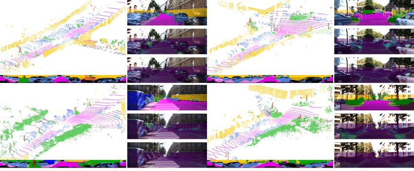
C. Qualitative Results D. Ablation Study
For the qualitative evaluation, Fig. 4 shows some sample In this ablative analysis, we investigate the individual
semantic segmentation and uncertainty results generated by contribution of each improvements over the original SalsaNet
SalsaNext on the Semantic-KITTI test set. model. Table II shows the total number of model parameters
In this figure, only for visualization purposes, segmented and FLOPs (Floating Point Operations) with the obtained
object points are also projected back to the respective camera mIoU scores on the Semantic-KITTI test set before and after
image. We, here, emphasize that these camera images have applying the kNN-based post processing (see section III-F).
not been used for training of SalsaNext. As depicted in As depicted in Table II, each of our contributions on
Fig. 4, SalsaNext can, to a great extent, distinguish road, SalsaNet has a unique improvement in the accuracy. The
car, and other object points. In Fig. 4, we additionally show post processing step leads to a certain jump (around 2%) in
the estimated epistemic and aleatoric uncertainty values the accuracy. The peak in the model parameters is observed
projected on the camera image for the sake of clarity. Here, when dilated convolution stack is introduced in the encoder,
the light blue points indicate the highest uncertainty whereas which is vastly reduced after adding the pixel-shuffle layers
darker points represent more certain predictions. In line with in the decoder. Combining the weighted cross-entropy loss
Fig. 3, we obtain high epistemic uncertainty for rare classes with Lovász-Softmax leads to the highest increment in the
such as other-ground as shown in the last frame in Fig. 4. We accuracy as the Jaccard index is directly optimized. We can
also observe that high level of aleatoric uncertainty mainly achieve the highest accuracy score of 59.5% by having only
appears around segment boundaries (see the second frame 2.2% (i.e. 0.15M) extra parameters compared to the original
in Fig. 4) and on distant objects (e.g. last frame in Fig. 4). SalsaNet model. Table II also shows that the number of
In the supplementary video1 , we provide more qualitative FLOPs is correlated with the number of parameters. We note
results. that adding the epistemic and aleatoric uncertainty compu-
tations do not introduce any additional training parameter
1 https://youtu.be/MlSaIcD9ItU since they are computed after the network is trained.
Fig. 4. Sample qualitative results showing successes of our proposed SalsaNext method [best view in color]. At the bottom of each scene, the range-view
image of the network response is shown. Note that the corresponding camera images on the right are only for visualization purposes and have not been
used in the training. The top camera image on the right shows the projected segments whereas the middle and bottom images depict the projected epistemic
and aleatoric uncertainties, respectively. Note that the lighter the color is, the more uncertain the network becomes.Processing Time (msec)
[10] B. Wu, X. Zhou, S. Zhao, X. Yue, and K. Keutzer, “Squeezesegv2:
CNN kNN Total Speed (fps) Parameters FLOPs Improved model structure and unsupervised domain adaptation for
RangeNet++ [7] 63.51 2.89 66.41 15 Hz 50 M 720.96 G road-object segmentation from a lidar point cloud,” in ICRA, 2019.
SalsaNet [1] 35.78 2.62 38.40 26 Hz 6.58 M 51.60 G [11] Y. Wang, T. Shi, P. Yun, L. Tai, and M. Liu, “Pointseg: Real-time
SalsaNext [Ours] 38.61 2.65 41.26 24 Hz 6.73 M 125.68 G semantic segmentation based on 3d lidar point cloud,” CoRR, 2018.
[12] E. Shelhamer, J. Long, and T. Darrell, “Fully convolutional networks
TABLE III for semantic segmentation.” PAMI, 2016.
RUNTIME PERFORMANCE ON THE S EMANTIC -KITTI TEST SET [13] C. Zhang, W. Luo, and R. Urtasun, “Efficient convolutions for real-
time semantic segmentation of 3d point clouds,” in 3DV, 2018.
[14] O. Ronneberger, P.Fischer, and T. Brox, “U-net: Convolutional net-
works for biomedical image segmentation,” in Medical Image Com-
puting and Computer-Assisted Intervention, 2015, pp. 234–241.
E. Runtime Evaluation [15] C. R. Qi, H. Su, K. Mo, and L. J. Guibas, “Pointnet: Deep learning
on point sets for 3d classification and segmentation,” in CVPR, 2017.
Runtime performance is of utmost importance in au- [16] C. R. Qi, L. Yi, H. Su, and L. J. Guibas, “Pointnet++: Deep
tonomous driving. Table III reports the total runtime perfor- hierarchical feature learning on point sets in a metric space,” in NIPS,
mance for the CNN backbone network and post-processing 2017.
[17] L. Landrieu and M. Simonovsky, “Large-scale point cloud semantic
module of SalsaNext in contrast to other networks. To obtain segmentation with superpoint graphs,” in CVPR, 2018.
fair statistics, all measurements are performed using the [18] C. R. Qi, W. Liu, C. Wu, H. Su, and L. J. Guibas, “Frustum pointnets
entire Semantic-KITTI dataset on the same single NVIDIA for 3d object detection from RGB-D data,” CoRR, 2017.
[19] Y. Zhou and O. Tuzel, “Voxelnet: End-to-end learning for point cloud
Quadro RTX 6000 - 24GB card. As depicted in Table III, our based 3d object detection,” in CVPR, 2018.
method clearly exhibits better performance compared to, for [20] L. P. Tchapmi, C. B. Choy, I. Armeni, J. Gwak, and S. Savarese,
instance, RangeNet++ [7] while having 7× less parameters. “Segcloud: Semantic segmentation of 3d point clouds,” in 3DV, 2017.
[21] F. J. Lawin, M. Danelljan, P. Tosteberg, G. Bhat, F. S. Khan, and
SalsaNext can run at 24 Hz when the uncertainty computation M. Felsberg, “Deep projective 3d semantic segmentation,” CoRR,
is excluded for a fair comparison with deterministic models. 2017. [Online]. Available: http://arxiv.org/abs/1705.03428
Note that this high speed we reach is significantly faster [22] H. Su, V. Jampani, D. Sun, S. Maji, E. Kalogerakis, M. Yang,
and J. Kautz, “Splatnet: Sparse lattice networks for point cloud
than the sampling rate of mainstream LiDAR sensors which processing,” in CVPR, 2018.
typically work at 10 Hz [39]. Fig. 1 also compares the [23] R. Alexandru Rosu, P. Schütt, J. Quenzel, and S. Behnke, “LatticeNet:
overall performance of SalsaNext with the other state-of- Fast Point Cloud Segmentation Using Permutohedral Lattices,” arXiv
e-prints, p. arXiv:1912.05905, Dec. 2019.
the-art semantic segmentation networks in terms of runtime, [24] C. Xu, B. Wu, Z. Wang, W. Zhan, P. Vajda, K. Keutzer, and
accuracy, and memory consumption. M. Tomizuka, “Squeezesegv3: Spatially-adaptive convolution for effi-
cient point-cloud segmentation,” 2020.
V. C ONCLUSION [25] Y. Zeng, Y. Hu, S. Liu, J. Ye, Y. Han, X. Li, and N. Sun, “Rt3d:
Real-time 3-d vehicle detection in lidar point cloud for autonomous
We presented a new uncertainty-aware semantic segmen- driving,” IEEE RAL, vol. 3, no. 4, pp. 3434–3440, Oct 2018.
tation network, named SalsaNext, that can process the full [26] M. Simon, S. Milz, K. Amende, and H. Gross, “Complex-yolo: Real-
time 3d object detection on point clouds,” CoRR, 2018.
360◦ LiDAR scan in real-time. SalsaNext builds up on the [27] I. Alonso, L. Riazuelo, L. Montesano, and A. C. Murillo, “3d-mininet:
SalsaNet model and can achieve over 14% more accuracy. Learning a 2d representation from point clouds for fast and efficient
In contrast to previous methods, SalsaNext returns +3.6% 3d lidar semantic segmentation,” 2020.
[28] Y. Gal and Z. Ghahramani, “Dropout as a bayesian approximation:
better mIoU score. Our method differs in that SalsaNext can Representing model uncertainty in deep learning,” in ICML, 2016.
also estimate both data and model-based uncertainty. [29] A. Loquercio, M. Segú, and D. Scaramuzza, “A general framework
for uncertainty estimation in deep learning,” RA-L, 2020.
R EFERENCES [30] D. Feng, L. Rosenbaum, and K. Dietmayer, “Towards safe autonomous
driving: Capture uncertainty in the deep neural network for lidar 3d
[1] E. E. Aksoy, S. Baci, and S. Cavdar, “Salsanet: Fast road and vehicle vehicle detection,” in ITSC. IEEE, 2018, pp. 3266–3273.
segmentation in lidar point clouds for autonomous driving,” in IEEE [31] E. Ilg, O. Cicek, S. Galesso, A. Klein, O. Makansi, F. Hutter, and
Intelligent Vehicles Symposium (IV2020), 2020. T. Brox, “Uncertainty estimates and multi-hypotheses networks for
[2] M. Berman, A. Rannen Triki, and M. B. Blaschko, “The lovász- optical flow,” in ECCV, 2018, pp. 652–667.
softmax loss: A tractable surrogate for the optimization of the [32] B. Zhang and P. Wonka, “Point cloud instance segmentation using
intersection-over-union measure in neural networks,” in CVPR, 2018. probabilistic embeddings,” CoRR, 2019.
[3] J. Behley, M. Garbade, A. Milioto, J. Quenzel, S. Behnke, C. Stach- [33] K. He, X. Zhang, S. Ren, and J. Sun, “Deep residual learning for
niss, and J. Gall, “SemanticKITTI: A Dataset for Semantic Scene image recognition,” in CVPR, 2016, pp. 770–778.
Understanding of LiDAR Sequences,” in ICCV, 2019. [34] M. D. Zeiler and R. Fergus, “Visualizing and understanding convolu-
[4] A. Kendall, V. Badrinarayanan, and R. Cipolla, “Bayesian segnet: tional networks,” CoRR, vol. abs/1311.2901, 2013.
Model uncertainty in deep convolutional encoder-decoder architectures [35] X. Li, S. Chen, X. Hu, and J. Yang, “Understanding the disharmony
for scene understanding,” arXiv preprint arXiv:1511.02680, 2015. between dropout and batch normalization by variance shift,” 2018.
[5] R. P. K. Poudel, S. Liwicki, and R. Cipolla, “Fast-scnn: Fast semantic [36] J. Gast and S. Roth, “Lightweight probabilistic deep networks,” in
segmentation network,” CoRR, vol. abs/1902.04502, 2019. CVPR, 2018, pp. 3369–3378.
[6] B. Wu, A. Wan, X. Yue, and K. Keutzer, “Squeezeseg: Convolutional [37] M. Tatarchenko, J. Park, V. Koltun, and Q. Zhou, “Tangent convolu-
neural nets with recurrent crf for real-time road-object segmentation tions for dense prediction in 3d,” in CVPR, 2018.
from 3d lidar point cloud,” ICRA, 2018. [38] Q. Hu, B. Yang, L. Xie, S. Rosa, Y. Guo, Z. Wang, N. Trigoni, and
[7] A. Milioto, I. Vizzo, J. Behley, and C. Stachniss, “RangeNet++: Fast A. Markham, “Randla-net: Efficient semantic segmentation of large-
and Accurate LiDAR Semantic Segmentation,” in IROS, 2019. scale point clouds,” 2019.
[8] Y. Guo, H. Wang, Q. Hu, H. Liu, L. Liu, and M. Bennamoun, “Deep [39] A. Geiger, P. Lenz, and R. Urtasun, “Are we ready for autonomous
learning for 3d point clouds: A survey,” CoRR, 2019. driving? the kitti vision benchmark suite,” in CVPR, 2012.
[9] W. Shi, J. Caballero, F. Huszár, J. Totz, A. P. Aitken, R. Bishop,
D. Rueckert, and Z. Wang, “Real-time single image and video super-
resolution using an efficient sub-pixel convolutional neural network,”
CoRR, vol. abs/1609.05158, 2016.You can also read