Integrated Design of Unmanned Aerial Mobility Network: A Data-Driven Risk-Averse Approach
←
→
Page content transcription
If your browser does not render page correctly, please read the page content below
Integrated Design of Unmanned Aerial Mobility Network: A
                                                                       Data-Driven Risk-Averse Approach
arXiv:2004.13000v1 [math.OC] 28 Apr 2020

                                                                                                                                  ∗ 1
                                                                  Wenjuan Hou1 , Tao Fang2 , Zhi Pei2 , and Qiao-Chu He

                                                           1
                                                               School of Business, Southern University of Science and Technology
                                                     2
                                                         Department of Industrial Engineering, Zhejiang University of Technology

                                                                                           April 29, 2020

                                                                                             Abstract

                                                    The real challenge in drone-logistics is to develop an economically-feasible Unmanned Aerial
                                                 Mobility Network (UAMN). In this paper, we propose an integrated airport location (strate-
                                                 gic decision) and routes planning (operational decision) optimization framework to minimize
                                                 the total cost of the network, while guaranteeing flow constraints, capacity constraints, and
                                                 electricity constraints. To facility expensive long-term infrastructure planning facing demand
                                                 uncertainty, we develop a data-driven risk-averse two-stage stochastic optimization model based
                                                 on the Wasserstein distance. We develop a reformulation technique which simplifies the worst-
                                                 case expectation term in the original model, and obtain a fractable Min-Max solution procedure
                                                 correspondingly. Using Lagrange multipliers, we successfully decompose decision variables and
                                                 reduce the complexity of computation.
                                                    To provide managerial insights, we design specific numerical examples. For example, we find
                                                 that the optimal network configuration is affected by the “pooling effects” in channel capacities.
                                                 A nice feature of our DRO framework is that the optimal network design is relatively robust
                                                 under demand uncertainty. Interestingly, a candidate node without historical demand records
                                                 can be chosen to locate an airport. We demonstrate the application of our model for a real
                                                 medical resources transportation problem with our industry partner, collecting donated blood
                                                 to a blood bank in Hangzhou, China.
                                                 Keywords: facility location, unmanned aerial vehicles, distributionally robust opti-
                                                 mization, data-driven, risk-averse

                                           ∗
                                               Corresponding author: heqc@sustech.edu.cn

                                                                                                 1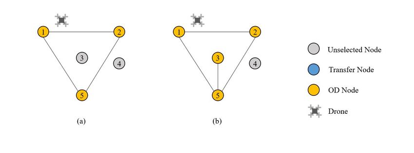
1        Introduction

Traditional logistics service based on land vehicles is facing emerging challenges such as increasing
labor costs and traffic congestions, in contrast to growing logistics demand and rising customer
expectation of delivery service quality. This is particularly the case for certain sectors in urban
logistics, e.g., grocery or fresh products logistics, healthcare resources and products, and emer-
gency/humanitarian logistics, in which context the goods are to be delivered within hours. Drones
logistics, as complement to land vehicles, can fill in the gaps in the aforementioned context and is
already becoming a reality. Although drone logistics cannot replace land vehicles entirely due to
relatively higher cost and limited capacity, it certainly outperforms the latter in terms of efficiency
(point-to-point delivery directly from origins to destinations) and accessibility (patching geographic
holes such as islands and mountainous areas). However, apart from certain showcase examples of
drone delivery, it is not until recently that the technology (e.g., affordable AI-enabled navigation)
and policy conditions         1   are prepared. Therefore, industry giants       2   start prototype programs, but
they quickly identify that the real challenge to implement economically-feasible drone-logistics at
large scale, is to develop an unmanned aerial mobility network (UAMN): a data-and algorithm-
driven service platform to coordinate the deployment of infrastructures (airports, charging stations,
etc.) as well as the operations management of drones fleets (route planning, on-demand delivery
scheduling,etc.). Therefore, the industry needs motivate our research in designing such an UAMN,
which is clearly relevant to the operations research/management community.

         The existing literature on drone logistics pivots heavily on solving vehicle routing problems,
with a few exceptions related to network design, e.g., [3, 17]. We depart from the on-demand
scheduling/vehicle routing problems, and focus on route planning. Thus, our model is most closely
related to the hub-location model for air transportation network design [23] and the reference
therein. The rationale is that aerial routes cannot be optimized on demand, since any route has
to be reported to the regulating agency (such as FAA in the US) for prior approval. Once the
routes are determined, the service platform can decide the frequency and volume en route but
cannot adjust the fixed itineraries at will. In other words, the real problem of UAMN design is
more analogous to building a highway network or urban bus network rather than vehicle routing
    1
        The Federal Aviation Administration (FAA) said on Friday, August 2 that it has approved the drone’s first flight
beyond the line-of-sight of the operator.
   2
     At the end of March 2018, Amazon was patented that express drones can recognize and respond to waving arms,
pointing, flashing lights and voice, etc.

                                                             2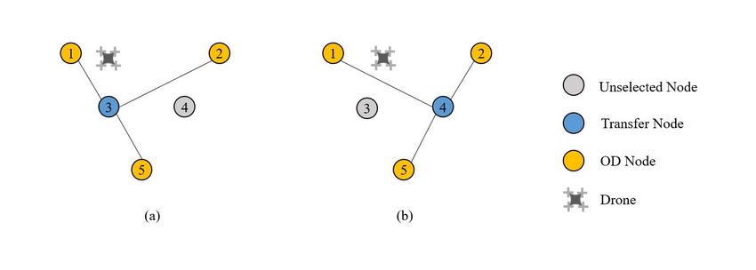
problems.

        In this paper, we address the following research question: how to design an UAMN under
demand uncertainty while integrating macro-level strategic decisions (infrastructure planning de-
cisions, e.g., airport location and capacity, as well as route planning) and micro-level operational
decisions (transportation decisions, battery charging feasibility, etc.). We choose a data-driven dis-
tributionally robust optimization (DRO) framework to support the costly long-term infrastructure
planning decisions due to demand uncertainty.

        In this paper, we proposed a novel integrated airport location and routes planning model for
UAMN, using a Wasserstein-distance based DRO framework. Our objective is to mininize the
aggregate cost, with airport capacity constraints, flow-conservation constraints, battery capacity
constraints, and satisfy all demands. We do not keep track of individual drones, but focus on trans-
portation volumes (similar to bus frequency). We also abstract away from the dynamic charging
process, and ensure that total electricity boosts can last the entire itineracy on a cyclic basis.

        We allow for mis-calibration of demand distribution by considering its ambiguity set based on
the Wasserstain distance. Such Wasserstain distance-based distributionally robust optimization is
flexible not only in fully utilizing historical demand data, but also risk-averse in the sense that inac-
curate estimate for distribution leads to sub-optimal solution, e.g., [30]. Such a decision framework
is suitable for our problem context because costly long term infrastructure planning decisions are
made under demand uncertainty with limited data. We also reformulate the problem to maintain
computational tractability. Numerical examples are proposed to generate managerial insights man-
agerial insights concerning the strategic location decisions. Finally, we apply our model to solve a
representative problem for our industry partner Xunyi3 which is the first operating aerial logistics
company approved by the Civil Aviation Administration of China.

        Our specific contributions are:

        1. We identify and conceptualize the key challenge in drone logistics as the UAMN design
problem. Motivated by our industry partner, we focus on “building aerial highway” rather than
solving vehicle routing problems.
   3
       On 2019-10-17, our industry partner was issued a “specific unmanned aerial vehicle commissioning letter” and
“unmanned aerial vehicle logistics distribution business license”from the Civil Aviation Administration of China,
the first approval of its kind in China (http://chinaplus.cri.cn/news/china/9/20191017/368089.html). In contrast,
Amazon submitted FAA Approval for drone delivery on August 2019 and “there is no set timeline for approval”
(https://www.aviationtoday.com/2019/08/09/following-wing-ups-amazon-seeks-approval-prime-air-drone-delivery/).

                                                          3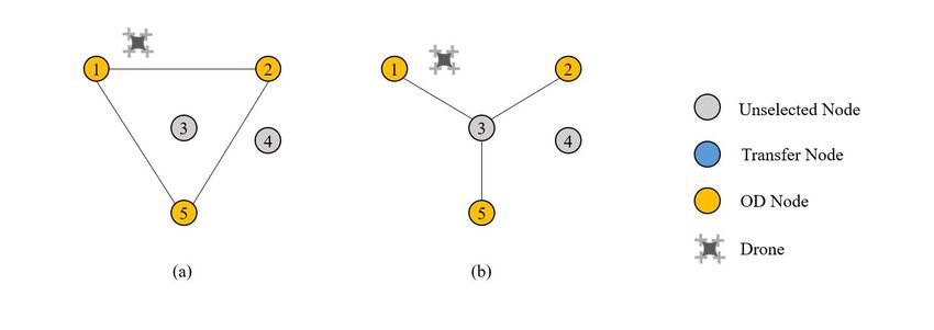
2. We apply the Wasserstain distance-based distributionally robust optimization framework
to facilitate data-driven decision making for both network design and operations management. We
also develop computational technique in reformulating the complex problem into tractable models.

    3. Through carefully designed numerical examples, we generate managerial insights towards
the strategic infrastructure planning decisions.

    4. Finally, in collaboration with our industry partner, we apply our model to solve a real
problem, delivering healthcare resources (blood and blood products) between blood collection sta-
tion and the blood bank in densely populated urban areas. We summarize this application in a
representative case study.

    The rest of this paper is organized as follows. Section 2 reviews relevant literature. Section 3
introduces our model setup. In Section 4, we carry out the analysis. In Section 5, we describe our
computational method, and provide numerical examples. Section 6 concludes this paper with a
discussion of future research directions.

2    Related Work

There is growing research interest in evaluating the economic efficiency in drone logistics, for ex-
ample, in a hybrid truck-and-drone model, e.g. [1, 11, 18]. [5] demonstrated the improvement in
efficiency this way, by combining a theoretical analysis in the Euclidean plane with real-time nu-
merical simulations on a road network. [20] used a branch-and-bound approach to solve the TSP-D
in which at each node the approximate lower bound is given by a dynamic program. [19] are first
to study the mothership and drone routing problem (MDRP) which is a more generalized TSP.
However, the existing literature ignores the key challenge in drone-logistics, which is the UAMN
design problem, so we focus our research on “building aerial highway”.

    The network design/facility location optimization have been studied extensively in the oper-
ations research community. [23] study a reliable hub location model, by exploiting the structural
properties of the problem, they introduce a tractable mixed-integer linear program reformulation
and develop a constraint generation method to accelerate the solution procedure. [2] develop a
two-stage RO reliable p-median facility location model to minimize the weighted cost in normal
and disruption scenarios. [7, 8] develop a continuum approximation (CA) model aiming to minimize
the overall expected total cost in normal and failure/disruption scenarios. Based on [2, 7, 8], [13]

                                                   4
develop a stylized continuous model, and investigate the impact of misestimating the disruption
probability. [14] present a model that allows disruptions to be correlated with an uncertain joint
distribution. And a distributionally robust optimization is applied to minimize the expected cost
under the worst-case distribution with given marginal disruption probabilities. [15] aid to locate
battery-swapping infrastructure and choose its capacity along an existing network of freeways with
by using limited information of demand, e.g., mean, variance, and develop a chance-constraint ro-
bust optimization model. In this paper, we solve the integrated problem of both facility location
and network design, fully utilizing the historical data, and develop a Wasserstain-distance robust
optimization model.
In addition, UAMN design problems can also get some inspiration from the traditional airline
operation management. [9] introduces a new approach to accurately calculate and minimize the
cost of propagated delay in a framework that integrates aircraft routing and crew pairing. [10]
extends the approach of [9] by proposing two new algorithms that achieve further improvements in
delay propagation reduction via the incorporation of stochastic delay information. [28] introduces
the flight routes addition/deletion problem and compares three different methods to analyze and
optimize the algebraic connectivity of the air transportation network. [25] aims to manage the
increasing complexity of traffic flow in the airspace and present a traffic flow model called the Large-
Capacity Cell Transmission Model in which the integer program is relaxed to a linear program for
computational efficiency. [27] inherits this problem, rewrite it in a standard linear programming
and analyze the total unimodular property of the constraint matrix. The authors prove that a
simplex related method guarantees the solutions to be optimal. [21] focuses on the formulation of
fixed finial time multiphase optimal control problem with energy consumption as the performance
index for a multirotor eVTOL aircraft. [24] proposes mathematical models for commercial transport
service providers to decide which type of schedule to offer, how to dispatch the fleet and schedule
operations, based on simulated market demand, such that profits is maximized. However, this
stream of research usually step from a small segmentation of aerial mobility network and develop
a heuristic approach. To generate systematic conclusions and managerial insight, our basic model
is somewhat stylized and can be solved via an exact approach.
Stochastic programming can effectively describe many decision-making problems in uncertain
environments. We finally review the solution methodology for stochastic programming in the
network design and facility location literature. We do not post distributional assumptions on
demand uncertatinty (typically required for stochastic programming with chance constraints). Note
5that the solution framework we used in this paper has been also applied to the unit commitment
problems [26, 29]. The classic solution to such stochastic program is by scenario sampling [4],
or robust optimization [15]. [12] proposed a two-stage robust optimization model to address the
network constrained unit commitment problem under uncertainty. [16] studies the storage and
distribution problem of medical supplies by implementing stochastic optimization approach. In
this paper, our solution approach is most related to [30] which studied a data-driven risk-averse
stochastic optimization approach with Wasserstein distance for the general distribution case. They
reformulated the risk-averse two-stage stochastic optimization problem to a traditional two-stage
robust optimization problem via using Wasserstein distance. We apply this framework to our
UAMN design problem, and develop an integrated data-driven risk-verse model.
3 Model
Demand uncertainty. We use bk (ω) to denote the demand volume for the kth O-D pair. Con-
sidering that there is uncertainty in the demand, bk (ω) is a random variable, wherein each ω
corresponds to a random draw from some sample space Ω. We can omit ω in bk (ω) and denote
demand volume by bk . In fact, the actual demand distribution for bk is unknown at the stage of in-
frastructure planning, e.g., airport location, route and channel design, etc. An inaccurate estimate
of the demand distribution may lead to suboptimal infrastructure investment decisions, and thus,
it is desirable to adopt a distributionally robust optimization framework without picking a fixed
distribution ex ante. At this stage, we have no restriction for the demand distribution other than
that it is bounded with an upper bound (denoted by Wk+ ) and a lower bound (denoted by Wk− ).
Meanwhile, to utilize the historical demand data, we adopt a data-driven approach wherein the
true distribution should be “close” to the reference distribution empirically estimated from data,
in the sense of “Wasserstein distance metric” which has been utilized in [30], [6]. We will specify
the detailed setup in the analysis.
Unmanned aerial mobility network. We use a set V to denote all nodes in the UAMN,
which includes supply nodes (“origin”, i.e., warehouses and distribution centers), demand nodes
(“destination”, i.e., customer) and transfer nodes (i.e., transfer airport). Goods are delivered from
origins to destinations though the UAMN, enabled by a fleet of orchestrated drones via optimization
algorithms. We represent a delivery demand k by its origin Ok and destination Dk , and use a set
K to denote all O-D pairs. A pair of nodes in the UAMN constitute a route, represented by the arc
6set A in the network. A “route” connecting two nodes consists of multiple “channels”, i.e., aerial
corridors that confines the trajectories of drones, similar to a highway consisting of multiple lanes.
In addition, there could be multiple types of channels (fast vs. slow) and we denote the channel
type by a set T . A node with a non-zero demand indicates an airport, at which drones can pick up
or deliver goods, as well as lay over for charging. A node is referred to as a “transfer airport”, if
drones can charge but not pick up or deliver at the node. We use a binary decision variable zi to
decide whether an airport should be in potential location i. In this paper, we focus on the UAMN
design and do not keep track of the moving path of individual drones.
Flow constraints. For a particular O-D pair (denoted by index k), we use set V − Ok − Dk
to denote its transfer nodes. We represent the demand volume of k by bk . We use xkji to denote
transportation volume en route (i, j) for kth O-D pair. For a particular O-D pair (denoted by
index k), at a pick-up location (origin node), the net transportation volume out of the node is bk
(flow-out volume subtracted by the flow-in volume):
X X
xkij (ω) − xkji (ω) = bk (ω), ∀k ∈ K, ∀i ∈ Ok .
j:(i,j)∈A j:(i,j)∈A
At a pick-up location (demand node), the net transportation volume out of the node is −bk (flow-out
volume subtracted by the flow-in volume):
X X
xkij (ω) − xkji (ω) = −bk (ω), ∀k ∈ K, ∀i ∈ Dk .
j:(i,j)∈A j:(i,j)∈A
At a pick-up location (transfer node), the net transportation volume out of the node is 0 (flow-out
volume subtracted by the flow-in volume):
X X
xkij (ω) − xkji (ω) = 0, ∀k ∈ K, ∀i ∈ V − Ok − Dk .
j:(i,j)∈A j:(i,j)∈A
Capacity constraints. We first make strategic decisions by locating airports. An airport is
capacitated due to (1) limited “port” for landing and take-off as well as (2) limited parking spaces,
and the capacity for the airport at location i is wi . As we have described, a route may consist of
multiple channels of type t, we assume that the capacity of a type t channel en route (i, i) is utij .
t to decide how many channels of type t should be invested
We use an integer decision variable yij
in a potential route (i, j).
For a route denoted by an arc (i, j) in the UAMN, the total net transportation volume through
this route cannot exceed total capacity volume. Hence, we set this constraint to limit transportation
7volume. The left side represents the sum of transportation volume over all O-D pairs, while the
right hand represents the sum of capacity volume over all channel types.
X X
xkij (ω) ≤ utij yij
t
, ∀(i, j) ∈ A.
k∈K t∈T
For a location node denoted by i, if zi = 1 (an airport should be), its capacity volume is wi , if
zi = 0 (an airport should not be), its capacity is unlimited. We integrate these two possible cases
together and set the constraint as follows, wherein M is a large number:
X X X X
xkij (ω) + xkji (ω) ≤ wi zi + M (1 − zi ), ∀i ∈ V.
k∈K j:(i,j)∈A k∈K j:(i,j)∈A
Notice that the capacity constraints both at the airport and en route between nodes relate the
location decisions {z}’s, network design decisions {y}’s, and the transportation decisions {x}’s.
Therefore, the strategic (infrastructure) decisions are intertwined with the operation decisions
(transportation or scheduling). This is a salient feature of UAMN design in terms of the inte-
gration of different decision hierarchies.
Battery capacity constraints. We use lij to denote the consumption of electricity quantity
en route (i, j), while L denotes a lumpsum boost in battery level upon a charging completion. For
a particular O-D pair (denoted by index k), the total battery consumption is less than the total
battery charged. We set the electricity constraints as follows, wherein the first term is the sum
of battery consumption over all routes, and the second term is the sum of electricity charged over
all routes. The amount of electricity charged is only included in the summation when the route is
chosen (x 6= 0) and the airport (charging station) is located (z = 1). This constraint means that
there is enough total charge to reach the charge-discharge balance in one operating period.
X X
lij xkij (ω) ≤ bk zi L, ∀k ∈ K,
(i,j)∈A (i,j)∈A
We also abstract away from the dynamic charging process to focus on the charging location:
We assume that drones can only get charged at airports (including transfer ones), and we ensure
that total electricity boosts (can charge multiple times) can last the entire itineracy, on a cyclic
basis. As we focus on strategic level planning, we do not keep track of the battery level for individual
drones (also computationally intractable).
Objective. The aggregate costs consist of transportation cost, aerial channel cost, airport
infrastructure cost, and airport capacity cost. We use Ctkij to denote the cost to transport unit
8volume cargo for the kth O-D pair en route (i, j), Cdtij to denote the cost to set up a channel of
type t en route (i, j), Cfj to denote the infrastructure cost to locate an airport for the jth location,
and Csj to denote the cost to set unit volume capacity for the jth location. We sum up all these
costs over all routes, all locations, and all types. Our objective function takes the form as follows:
X X X X X X
min Ctkij xkij (ω) + Cdtij yij
t
+ Cfj zj + Csj wj zj .
k∈K (i,j)∈A t∈T (i,j)∈A j∈V j∈V
Our model is systematic by integrating all kinds of costs.
To summarize, we solve the following mixed integer program:
• Objective:
X X X X X X
min Ctkij xkij (ω) + Cdtij yij
t
+ Cfj zj + Csj wj zj .
k∈K (i,j)∈A t∈T (i,j)∈A j∈V j∈V
• Flow constraints:
X X
xkij (ω) − xkji (ω) = bk (ω), ∀k ∈ K, ∀i ∈ Ok . (1)
j:(i,j)∈A j:(i,j)∈A
X X
xkij (ω) − xkji (ω) = −bk (ω), ∀k ∈ K, ∀i ∈ Dk . (2)
j:(i,j)∈A j:(i,j)∈A
X X
xkij (ω) − xkji (ω) = 0, ∀k ∈ K, ∀i ∈ V − Ok − Dk . (3)
j:(i,j)∈A j:(i,j)∈A
• Capacity constraints:
X X
xkij (ω) ≤ utij yij
t
, ∀(i, j) ∈ A. (4)
k∈K t∈T
X X X X
xkij (ω) + xkji (ω) ≤ wi zi + M (1 − zi ), ∀i ∈ V. (5)
k∈K j:(i,j)∈A k∈K j:(i,j)∈A
• Battery capacity constraints:
X X
lij xkij (ω) ≤ bk zi L, ∀k ∈ K, (6)
(i,j)∈A (i,j)∈A
9We summarize the nomenclature in this paper as follows:
A The set of all arcs in the network. V The set of all nodes in the network.
K The set of all O-D pairs in the network. T The set of all types of channels (e.g.,
fast, slow, etc.) in the arcs.
Ok The origin node for an O-D pair. Dk The destination node for an O-D pair.
bk The transportation demand for an O-D xkij Continuous variables for transportation
pair. volume.
t
yij Integer variables for number of channel utij Capacities of channel of type t at route
of type t at route (i, j). (i, j).
zi Binary decision variables for an airport wi Capacities for an airport at location i.
at location i.
L A lumpsum boost in battery level upon lij Energy/electricity consumed for route
a charging completion. (i, j).
Ctkij The cost to transport unit volume cargo Cdtij The cost to set up a channel of type t en
for the kth O-D pair en route (i, j). route (i, j).
Cfj The infrastructure cost to locate an air- Csj The cost to set unit volume capacity for
port for the jth location. the jth location.
4 Analysis and Computation Technique
4.1 Reformulations
We set up a two-stage model in last section, in which the first-stage makes decisions for locations
and channels and the second-stage makes decisions for transformation volume. Its second-stage
problem is as follows:
X X
Q(η, b) = min Ctkij xkij
x
k∈K (i,j)∈A
s.t. (1), (2), (3), (4), (5), (6)
where η = (z, y). We use η to vectorize decision variables of z and y.
10We can rewrite the Q(η, b) as follows:
min C T X
X
s.t. AX = B
DX ≤ E,
Where A, B, C, D, E are matric, and we give the detail definition of them in appendix.
Using traditional two-stage stochastic optimization framework in [22], we can formulate above
two-stage problem as follows:
X X X X
(SP ) min EP [Q(η, b)] + Cdtij yij
t
+ Cfj zj + Csj wj zj
η
t∈T (i,j)∈A j∈V j∈V
where P is the actual distribution of demand. However, P is usually unknown and the estimate
of it is different and inaccurate, i.e., historical demand data are not enough, future demand may
change. In addition, this model incorporates no risk averseness.
Considering that the cost to construct an new UAMN is expensive, the UAMN needs to
have a long-term utility under demand uncertainty. We choose the worst-case distribution in
the set defined by Wasserstein distance metric and consider a data-driven risk-averse stochastic
optimization formulation as follows:
X X X X
(DD − SP ) min max EPb [Q(η, b)] + Cdtij yij
t
+ Cfj zj + Csj wj zj
η Pb∈D t∈T (i,j)∈A j∈V j∈V
D = {Pb : dM (P0 , Pb) ≤ θ}
where P0 is the reference empirical distribution determined through historical data. dM is the
Wasserstein distance defined on two distributions. D is a confidence set of the true distribution by
confining dM less than or equal to θ which decides the size of D. On the one hand, we fully utilize
the historical demand data because D is a set near the reference distribution. On the other hand,
we use a set to estimate actual distribution rather than a concrete distribution. So our model is
both data-driven and risk-averse.
The aforementioned decision framework is known to have verified convergence property [30].
However, directly solving this two-stage risk-averse stochastic program is computationally challeng-
ing. Next, we start by reformulating the problem.
11Proposition 1. The problem DD − SP under D is equivalent to the following two-stage robust
optimization problem:
N
1 X X X X X
(RDD − SP ) min max[Q(η, b) − βρi (b)] + θβ + Cdtij yij
t
+ Cfj zj + Csj wj zj
η,β≥0 N b
i=1 t∈T (i,j)∈A j∈V j∈V
where ρi (b) = ρ(b, bi ).
We reformulate the original problem (DD − SP ) to a two-stage robust optimization problem
in Proposition 1. By finding the worst distribution of b in D, we eliminate the confidence set and
attain the expected value. The worst distribution of b is also discrete because Wasserstein distance
is used to capture the optimal transport between discrete distributions. The term βρi (b) can be
understood as a penalty about b. The value of β decides the confidence level of D. The other
terms remain the same as that in the original problem (DD − SP ). However, the subproblem is
still not linear because ρ is nonlinear, which has the absolute value. We will deal with ρ in the next
proposition.
Proposition 2. The problem RDD − SP is equivalent to the following Min-Max problem:
N
1 X j X X X X
(M aster) min $ (η, β) + θβ + Cdtij yij
t
+ Cfj zj + Csj wj zj
η,β≥0 N
j=1 t∈T (i,j)∈A j∈V j∈V
where η = (ω, z, y), and $j (η, β) is a (SUB) problem as follows:
K
(µi − µK+i )((Wi+ − bji )δi+ + (Wi− − bji )δi− + bji )
X
(Sub)$j (η, β) = max [−
δ + ,δ − ,µ,λ≥0
i=1
K
((Wi+ − bji )δi+ − (Wi− − bji )δi− ) − λT E]
X
−β
i=1
s.t. C T + µT A + λT D ≥ 0
δi+ , δi− ∈ {0, 1}
δi+ + δi− ≤ 1.
where Wi+ is the upper bound of bi , and Wi− is the lower bound of bi .
The salient difference between Proposition 1 and Proposition 2 is that we reformulate the
subproblem to a linear problem for a given first stage decision. We attain this subproblem by
using the dual form of Q(η, b), and linearizing ρi (b). This Min-Max problem is a traditional two-
stage robust problem in which the first stage is the master problem and the second stage is the
subproblem.
12Because we linearize the subproblem in proposition 2, this Min-Max problem is solvable. For
any y, z and β, we can calculate the corresponding optimal value of the subproblem. Hence, we can
calculate the optimal value of the master problem and optimal solutions to the decision variables
y and z. Because β is the unique optimal value for every θ, it suffices to obtain the value of b by
solving the subproblem for given β. The confidence interval (radius of the Wasserstein ball) can be
adjusted by choosing β.
4.2 Solution procedures
In the previous subsection, we have reformulated our model as a Min-Max problem. Because the
decision variables z and y occur both in the master problem and subproblem, they have to be solved
recursively. For given choices of y and z, the subproblem will be a tractable linear program. Then
we solve the entire integer optimization problem with respect to y and z. We describe the solution
procedures in this section with a sketch of the derivations. The readers are referred to Appendix
D for detailed derivations.
Step1. We notice that the matric E in the subproblem is composed of decision variables y
and z, so we decompose E. Then we collect terms with respect to y and z.
Step2. We notice that these decision variables y and z rely on µ and λ, respectively. However,
decision variables y and z are interdependent because constraints are comprised of µ and λ. By
using multiplier γ ≥ 0, we can eliminate the constraint. We can rewrite the master problem as
13follows:
N K
1 XX j
ψ= max min − [ (µi − µjK+i )((Wi+ − bji )δij+ + (Wi− − bji )δij− + bji )] (7)
δ + ,δ − ,µ,λ≥0 η,β≥0 N
j=1 i=1
N K
1 XX
+[− ((Wi+ − bji )δij+ − (Wi− − bji )δij− ) + θ]β
N
j=1 i=1
X
+ [{−(λ1 )j (wj − M ) + Cfj + Csj wj }zj − (λ1 )j M ]
j∈V
X X
+ {Cdtij − (λ2 )ij utij }yij
t
t∈T (i,j)∈A
N
X
+ {C T + (µj )T A + (λj )T D}γ j
j=1
s.t. δi+ , δi− ∈ {0, 1}
δi+ + δi− ≤ 1.
where λ1 represents the multiplier of constraints (5), λ2 represents the multiplier of constraints
(4), and λ3 represents the multiplier of constraints (6). So the multiplier λ can be separated by
λ = (λ2 T , λ1 T , λ3 T )T . λj1 is corresponding to jth sample of λ1 , λj2 is corresponding to jth sample
of λ2 , and λj3 is corresponding to jth sample of λ3 . λ1 is the mean of λj1 , and λ2 is the mean of
T T T
λj2 . So the multiplier λj can be separated by λj = (λj2 , λj1 , λj3 )T . (λ1 )j is the component in λ1
corresponding to zj . (λ2 )ij is the component in λ2 corresponding to yij .
Step3. We have eliminated the constraint by the above operation. We can notice that z and
y are related to the different part of λ. If we can successfully separate λ, then the decision of z and
the decision of y will be independent. By separating N T j T j T j
P
j=1 {C + (µ ) A + (λ ) D}γ , we rewrite
14the problem as follows:
N K
1 XX j
ψ = max min{− [ (µi − µjK+i )((Wi+ − bji )δij+ + (Wi− − bji )δij− + bji ) − (µj )T Aγ j ] (8)
δ + ,δ − ,µ β≥0 N
j=1 i=1
N X
K
1
((Wi+ − bji )δij+ − (Wi− − bji )δij− ) + θ]β}
X
+[−
N
j=1 i=1
N N
(λj1 )T D1 γ j + (λj3 )T D3 γ j }
X X X
+ max min{ [{−(λ1 )j (wj − M ) + Cfj + Csj wj }zj − (λ1 )j M ] +
λ1 ,λ3 ≥0 z
j∈V j=1 j=1
X X N
X
+ max min{[ {Cdtij − (λ2 )ij utij }yij
t
+ (λh2 )Tij (D2 )(ij) γ h ]}
t
λ2ij ≥0 yij
(i,j)∈A t∈T h=1
N
X
+ CT γj
j=1
s.t. δi+ , δi− ∈ {0, 1}
δi+ + δi− ≤ 1.
where D1 represents the coefficients in constraints (5), D2 represents the coefficients in constraints
(4), and D3 represents the coefficients in constraints (6). So the multiplier D can be separated by
D = (D2 T , D1 T , D3 T )T . (D2 )(ij) is a row of D2 corresponding to yij .
Step4. We have decomposed λ and D according to z and y. Given the proper multiplier value
of γ, solving decision variables of z and y are independent. Furthermore, we can separate y to yij ,
because every yij is only related to (λ2 )ij . We change the arrangement of sum and Max-Min, and
attain the formula of (8). We can notice that the original Min-Max problemd which contains all
decision variables has been divided into several independent Min-Max problem which contains a
smaller number of variables. We notice that y can be divided into yij because every yij is only
related to (λ2 )ij , but z can not be divided into zj because zj is related to λ1 . Given the value of γ,
every decision variable yij can be solved independently. In addition, given the value of γ, decision
variables z can be solved.
Step5. We must remember that the multiplier γ represents the condition C T + (µj )T A +
(λj )T D ≥ 0. So we just need to find a proper γ make this constraint hold, then the remained
computation is decreased dramatically, allowing us to conduct our numerical study later.
It is clear that any node with nonzero transportation volume should be an airport location. We
choose to check this constraint at the end of the algorithm to reduce the computation complexity.
The formula (8) takes advantage of tractability comparing to the Min-Max problem which contains
15all decision variables. For the original Min-Max problem, the complexity increases exponentially
in the size of z and y. Though z can not be divided into zj , the amount of computation for (8) is
dramatically decreased comparing to the Min-Max problem in last section because the size of y is
much larger than the size of z.
5 Numerical Examples and Case Study
5.1 Numerical examples
We propose numerical examples to generate managerial insights. In particular, we design the
example to isolate the effect of particular factors on the network configurations.
To streamline our numerical examples, we fix some basic model parameters throughout this
section unless specified otherwise. We need to give value to some important parameters, the node
set V , the confidence set parameter θ, the confidence level β = 1000, the number of channel type t,
and the range of channel decision variable y. we choose V = 5, θ = 100, β = 1000, N = 2, t = 1, y
is binary. The rest of the parameters are also carefully chosen within a reasonable range of values.
It suffices to choose N = 2 to deliver the main messages in the following numerical examples.
Demands are simulated by censored Gaussian distribution, with the upper bound and lower bound
chosen at triple the standard deviations above and below the mean, respectively. Similarly, we
carefully assign reasonable values to the location of nodes (and thus the pairwise distance between
them), the length of routes, as well as cost coefficients specified in Table 1.
Proposition 3. (Observation 1) The marginal decision of setting up an additional airport at a
particular candidate location depends crucially on both the infrastructure cost at and transportation
cost en route to the location.
In this numerical example, we fix all parameters and vary solely the parameters listed in
Table 1, one at a time. Not surprisingly, when we either increase the infrastructure cost at or
transportation cost en route to node 3, the optimality of airport location is to avoid node 3 and
choose node 4. This observation is intuitive. A direct implication is to decide whether to set
up airport in densely populated urban areas (low transportation costs due to proximity towards
demands). Nevertheless, it reflects a trade-off between infrastructure costs and transportation
costs in locating the airport, which also justifies the integration of two dimensions (location vs.
transportation) in the first place.
16Table 1: Transfer airport location
Optimal location for transit airport Node 3 Node 4
Airport infrastructure cost Cf4 =15000 Cf4 =8000
Airport capacity cost Cs4 =2 Cs4 =1
Channel cost Cdi4 =2000 Cdi4 =1200
Transportation cost Cti4 =12 Cti4 =10
Figure 1: Transfer airport location
Proposition 4. (Observation 2) The optimal network configuration depends jointly on infrastruc-
tural and transportation cost coefficients, the battery capacity constraints, as well as the pooling
effects in channel capacities.
In this numerical example, we fix all parameters and vary solely the parameters listed in Table
2, one at a time. When we either increase the channel cost at or transportation cost en routes
between nodes 1,2,5, the optimality of topology is to avoid triangle configuration and chooses
hub-and-spoken configuration. When we decrease battery capacity, it chooses hub-and-spoken
configuration. In particular, when battery capacity is small, the triangle configuration can never
be the optimal solution even if its cost is lower, because drones need to satisfy the charge-discharge
balance constraints. Finally, we briefly explain the pooling effects in channel capacities. In general,
we prefer a single high capacity channel rather than multiple low capacity channels due to economies
of scale. The centralized channel smooths out the demand uncertainty and increases the utilization
rate of the channel in general.
17Table 2: Topology
Optimal network design Triangle configuration Hub-and-spoken configuration
Channel cost Cd12 , Cd15 , Cd25 =1200 Cd12 , Cd15 , Cd25 =7000
Transportation cost Ct12 , Ct15 , Ct25 =10 Ct12 , Ct15 , Ct25 =30
Battery capacity L = 20 L = 10
Figure 2: Topology
Proposition 5. (Observation 3) The optimal network design is relatively robust under demand
uncertainty.
Notice that to switch from node 3 to node 4, we need to either increase the mean of demand by
six times or the standard deviation by ten times. In other words, the network configuration is less
sensitive towards the demand uncertainty, compared with other cost coefficients. This observation
echoes our choices of distributionally robust optimization framework to avoid suboptimal long-term
infrastructure and investment under a conservative and adversarial demand forecast.
Table 3: Effect of mean and variance
Optimal location for transit airport Node 3 Node 4
b12 N (50, 102 ) N (300, 102 )
b12 N (300, 102 ) N (300, 1002 )
Proposition 6. (Observation 4) A candidate node without historical demand records can be chosen
to locate an airport.
18Node 3 is chosen to locate an additional airport when we increase the upper bound of simulated
demand for O-D pair between node 1 and node 3. This observation is intuitive, because the size
of confidence set increases as the upper bound increases, leading to a new worst-case distribution.
A direct implication is to decide whether to setup airport close to potential future customers who
have never requested logistics service before.
Figure 3: Demand occurs with zero demand
We summarize our results in the following observations:
• The marginal decision of setting up an additional airport at a particular candidate location
depends crucially on both the infrastructure cost at and transportation cost en route to the
location.
• The optimal network configuration depends jointly on infrastructural and transportation
cost coefficients, the battery capacity constraints, as well as the pooling effects in channel
capacities.
• The optimal network design is relatively robust under demand uncertainty.
• A candidate node without historical demand records can be chosen to locate an airport.
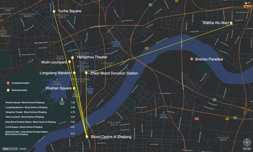
5.2 Case study
We perform a case study of UAMN design problem wherein the historical demand data is supplied by
our industry partner and the parameters are validated accordingly. We set β = 50, θ = 100, L = 18,
t = 1, y is binary. Transportation cost coefficients and battery consumption are proportional to
19their corresponding distance. Currently, airports are standardized products and we assume Cs is
homogeneous. We also set Cf and Cd identical across different locations in this study.
Table 4 provides historical demand data. There are 7 blood collection points in Hangzhou,
China, including Wushan Square, Longxiang Mansion, Hangzhou Theater, Wulin Courtyard, Zheyi
Blood Square, Yunhe Square, and Xiasha Wu Mart. All these 7 blood collection points supply
blood to blood bank for processing every day. We assume these 7 O-D pairs all take the upper
bound of demand as 25, and take the lower bound od demand as 0. We assume all other O-D pairs
take both the upper and the lower bound of demand as zeros in this pilot study.
Table 4: Blood Transportation Volume (kg) Depend on Location and Date
Date 2018/11/12 2018/11/13 2018/11/14 2018/11/15 2018/11/16 2018/11/17 2018/11/18
Wushan Square 0.4 3.1 4.6 3.1 1.3 6.4 1.5
Longxiang Mansion 4.3 4.2 4.4 4.93 5.2 9.9 8.4
Hangzhou Theater 1.3 1.2 1.4 0 0.8 3.2 0.5
Wulin Courtyard 5.2 9.9 5.5 5.9 0.5 12.3 12.7
Zheyi Blood Station 1 7 4.2 4.5 10.7 0 0
Yunhe Square 0 4.8 0 5.1 0 5.4 3.6
Xiasha Wu Mart 0 5.2 0 2.4 0 4.82 5.5
Distance data between all blood collection points and blood bank are given in the Appendix.
The main problem for the company is that Xiasha Wu Mart is far away from the blood bank,
which outlasts the battery capacity of their drones. Two options are to be evaluated: (A) Starting
from this remote location, the drone make a detour and transit at another location for charging.
This option incurs higher transportation costs due to the longer flight. We also need to decide the
transition point with sufficient capacity. (B) We set up an additional candidate airport, which can
potentially save the transportation cost but require additional infrastructure investment.
We solve this problem and attain the worst-case distribution of demand which are displayed in
Appendix. We can notice that the worst case distribution of demand is different from the original
sample demand. The value of demand can be their upper bound, lower bound, or themselves. This
table illustrates that our model considers the worst case under the confidence lever of β. Figure 4
20shows the blood transportation network design. Xiasha Wu mart and blood center are linked by
Zheyi blood donation station, rather than the candidate point Shenbo paradise, which means we
eventually choose option (A) or (B).
Figure 4: Blood transportation network
In summary, our model framework provides an exact approach to design a UAMN for drone
delivering. We can easily apply it on other real case studies related to drone delivering beyond
blood transportation.
6 Conclusion
In this paper, we propose an integrated facility location and network design problem, i.e., UAMN
design problem for drone logistics. To do this, we develop a risk-averse two-stage stochastic model
that is based on Wasserstein distance. We then develop a reformulation technique that simplifies
the worst-case expectation term in the original model, and obtain a Min-Max model correspond-
ingly. By using Lagrange multipliers, we successfully decompose decision variables and reduce the
computational complexity, allowing us to solve real-world instances under our model framework. A
few managerial observations are obtained through numerical examples. For example, we find that
the optimal network configuration is affected by the “pooling effects” in channel capacities. A nice
21feature of our DRO framework is that the optimal network design is relatively robust under demand
uncertainty. Interestingly, a candidate node without historical demand records can be chosen to
locate an airport. We next demonstrate the application of our model by providing a real problem
involving medical resources transportation with our industry partner.
References
[1] Agatz, N., P. Bouman, and M. Schmidt (2018). Optimization approaches for the traveling
salesman problem with drone. Transportation Science 52 (4), 965–981.
[2] An, Y., B. Zeng, Y. Zhang, and L. Zhao (2014). Reliable p-median facility location problem:
two-stage robust models and algorithms. Transportation Research Part B: Methodological 64,
54–72.
[3] Boutilier, J. J. and T. C. Chan (2019). Response time optimization for drone-delivered auto-
mated external defibrillators. arXiv preprint arXiv:1908.00149 .
[4] Calafiore, G. and M. C. Campi (2005). Uncertain convex programs: Randomized solutions and
confidence levels. Mathematical Programming 102 (1), 25–46.
[5] Carlsson, J. G. and S. Song (2017). Coordinated logistics with a truck and a drone. Management
Science 64 (9), 4052–4069.
[6] Chen, Z., M. Sim, and H. Xu (2019). Distributionally robust optimization with infinitely
constrained ambiguity sets. Operations Research 67 (5), 1328–1344.
[7] Chowdhury, S., A. Emelogu, M. Marufuzzaman, S. G. Nurre, and L. Bian (2017). Drones
for disaster response and relief operations: A continuous approximation model. International
Journal of Production Economics 188, 167–184.
[8] Cui, T., Y. Ouyang, and Z.-J. M. Shen (2010). Reliable facility location design under the risk
of disruptions. Operations research 58 (4-part-1), 998–1011.
[9] Dunbar, M., G. Froyland, and C.-L. Wu (2012). Robust airline schedule planning: Minimizing
propagated delay in an integrated routing and crewing framework. Transportation Science 46 (2),
204–216.
22[10] Dunbar, M., G. Froyland, and C.-L. Wu (2014). An integrated scenario-based approach for
robust aircraft routing, crew pairing and re-timing. Computers & Operations Research 45, 68 –
86.
[11] Jeong, H. Y., B. D. Song, and S. Lee (2019). Truck-drone hybrid delivery routing: Payload-
energy dependency and no-fly zones. International Journal of Production Economics 214, 220–
233.
[12] Jiang, R., M. Zhang, G. Li, and Y. Guan (2014). Two-stage network constrained robust unit
commitment problem. European Journal of Operational Research 234 (3), 751 – 762.
[13] Lim, M. K., A. Bassamboo, S. Chopra, and M. S. Daskin (2013). Facility location decisions
with random disruptions and imperfect estimation. Manufacturing & Service Operations Man-
agement 15 (2), 239–249.
[14] Lu, M., L. Ran, and Z.-J. M. Shen (2015). Reliable facility location design under uncertain
correlated disruptions. Manufacturing & Service Operations Management 17 (4), 445–455.
[15] Mak, H.-Y., Y. Rong, and Z.-J. M. Shen (2013). Infrastructure planning for electric vehicles
with battery swapping. Management Science 59 (7), 1557–1575.
[16] Mete, H. O. and Z. B. Zabinsky (2010). Stochastic optimization of medical supply location
and distribution in disaster management. International Journal of Production Economics 126 (1),
76–84.
[17] Moon, K. M., S. Chopra, S. K. Kim, and K. Lee (2019). Strategic location problem for
synchronized last-mile delivery with relaying drones. Article submitted to 2019 MSOM Supply
Chain SIG.
[18] Murray, C. C. and A. G. Chu (2015). The flying sidekick traveling salesman problem: Opti-
mization of drone-assisted parcel delivery. Transportation Research Part C: Emerging Technolo-
gies 54, 86–109.
[19] Poikonen, S. and B. Golden (2019). The mothership and drone routing problem. INFORMS
Journal on Computing.
[20] Poikonen, S., B. Golden, and E. A. Wasil (2019). A branch-and-bound approach to the
traveling salesman problem with a drone. INFORMS Journal on Computing 31 (2), 335–346.
23[21] Pradeep, P. and P. Wei (2019). Energy-efficient arrival with rta constraint for multirotor evtol
in urban air mobility. Journal of Aerospace Information Systems 16 (7), 263–277.
[22] Shapiro, A., D. Dentcheva, and A. Ruszczyski (2009). Lectures on stochastic programming:
Modeling and theory. SIAM 9.
[23] Shen, H., Y. Liang, and Z.-J. M. Shen (2019). Reliable hub location model for air transporta-
tion networks under random disruptions. Manufacturing & Service Operations Management,
Forthcoming.
[24] Shihab, S. A. M., P. Wei, D. Jurado, R. Mesa-Arango, and C. Bloebaum (2019, 06). By
schedule or on demand? - a hybrid operation concept for urban air mobility.
[25] Sun, D. and A. M. Bayen (2008). Multicommodity eulerian-lagrangian large-capacity cell
transmission model for en route traffic. Journal of guidance, control, and dynamics 31 (3), 616–
628.
[26] Wang, Q., Y. Guan, and J. Wang (2011). A chance-constrained two-stage stochastic pro-
gram for unit commitment with uncertain wind power output. IEEE Transactions on Power
Systems 27 (1), 206–215.
[27] Wei, P., Y. Cao, and D. Sun (2013). Total unimodularity and decomposition method for large-
scale air traffic cell transmission model. Transportation Research Part B: Methodological 53, 1 –
16.
[28] Wei, P., L. Chen, and D. Sun (2014). Algebraic connectivity maximization of an air trans-
portation network: The flight routes addition/deletion problem. Transportation Research Part
E: Logistics and Transportation Review 61, 13 – 27.
[29] Wu, H., M. Shahidehpour, Z. Li, and W. Tian (2014). Chance-constrained day-ahead schedul-
ing in stochastic power system operation. IEEE Trans. Power Syst. 29 (4), 1583–1591.
[30] Zhao, C. and Y. Guan (2018). Data-driven risk-averse stochastic optimization with wasserstein
metric. Operations Research Letters 46 (2), 262–267.
24Online Appendices
A Proof of Propositions
A.1 Proof for Proposition 1
Proof. We cite the lemma in [30] as follows:
Lemma 1. Assuming that there are N historical data samples ξ 1 , ξ 2 , · · · , ξ N which are i.i.d drawn
from the true distribution P, for any fixed first-stage decision x, we have
N
1 X
max EPb [Q(x, ξ)] = min max[Q(x, ξ) − βρ(ξ, ξ i )] + θβ
Pb∈D β≥0 N ξ
i=1
where x is the decision variables, and ξ is the sample which is uncertainty. Our decision
variables are η, and the demand bk is uncertainty. We substitute x as η, and substitute ξ as bk .
Then, the conclusion of proposition 1 is attained.
A.2 Proof for Proposition 2
Proof. We first take the dual of the formulation for the second-stage cost (i.e., Q(η, b) and combine
it with the second problem to obtain the following subproblem (denoted as SUB) corresponding to
each sample bj , j = 1, · · · , N :
(SU B)φj (η, β) = max {Q(η, b) − βρj (b)}
b
= max [min{(C T + µT A + λT D)X − µT B(b) − λT E} − βρj (b)]
b,µ,λ≥0 x
= max [−µT B(b) − λT E − βρj (b)]
b,µ,λ≥0
s.t. C T + µT A + λT D ≥ 0
We argue that C T + µT A + λT D ≥ 0. If argument does not hold, let X tend to positive infinity,
then (C T + µT A + λT D)X tends to negative infinity. Because we want to find max over µ, andλ,
C T + µT A + λT D ≥ 0 holds. The third equation holds because, if (C T + µT A + λT D)i = 0,
25then xi can be any nonnegative number, if (C T + µT A + λT D)i > 0, then xi will be zero, so
(C T + µT A + λT D)X = 0 always holds when we min over X.
− bji |, for a fixed λ,µ, obtain an optimal solution b to the problem (SUB):
PK
Let ρj (b) = i=1 |bi
K K K
|bi − bji | − λT E]
X X X
φj (η, β, λ, µ) = max[− µi bi + µK+i bi − β
b
i=1 i=1 i=1
So it can be observed that at least one optimal solution b∗ to the subproblem (SUB) satisfies
b∗i = Wi− ,b∗i = Wi+ ,or b∗i = bji , for each i = 1, 2, · · · , K, which indicate that for each i = 1, · · · , K,
the ith component of optimal solution b∗ can achieve its lower bound Wi− (δi+ = 0, δi− = 1), upper
bound Wi+ (δi+ = 1, δi− = 0), or the sample value bji (δi+ = δi− = 0).
Then, there exists an optimal solution b∗ of (SUB) satisfying the following constraints:
bi = (Wi+ − bji )δi+ + (Wi− − bji )δi− + bji , ∀i = 1, · · · , m,
δi+ + δi− ≤ 1, δi+ , δi− ∈ {0, 1}, ∀i = 1, · · · , m.
We can linearize the φj (η, λ, µ) as:
K K
|bi − bji | − λT E]
X X
j
φ (η, β, λ, µ) = max[− (µi − µK+i )bi − β
b
i=1 i=1
K
(µi − µK+i )((Wi+ − bji )δi+ + (Wi− − bji )δi− + bji )
X
= max[−
b
i=1
K
|(Wi+ − bji )δi+ + (Wi− − bji )δi− | − λT E]
X
−β
i=1
K
(µi − µK+i )((Wi+ − bji )δi+ + (Wi− − bji )δi− + bji )
X
= max[−
b
i=1
K
((Wi+ − bji )δi+ − (Wi− − bji )δi− ) − λT E]
X
−β
i=1
26The (SUB) can be described as follows:
K
(µi − µK+i )((Wi+ − bji )δi+ + (Wi− − bji )δi− + bji )
X
$j (η, β) = max [−
δ + ,δ − ,µ,λ≥0
i=1
K
((Wi+ − bji )δi+ − (Wi− − bji )δi− ) − λT E]
X
−β
i=1
s.t. C T + µT A + λT D ≥ 0
δi+ , δi− ∈ {0, 1}
δi+ + δi− ≤ 1.
B Matrix Definitions
The second-stage problem Q(η, b) is:
min C T X
X
s.t. AX = B
DX ≤ E,
• B = (bT , −bT , 0T )T ,b = (b1 , b2 , · · · , bK )T . B is a vector, and its size is determined by K.
• A is a matrix composed by coefficient before X in constraints (1),(2),(3). The number of
row is determined by the number of constraints (1) (2) (3), and the number of column is
determined by the size of vector X, i.e. it is equal to the number of elements in vector X.
• D is a matrix composed by coefficient before X in constraints (4),(5),(6). The number of
row is determined by the number of constraints (4) (5) (6), and the number of column is
determined by the size of vector X, i.e. it is equal to the number of elements in vector X.
• E is a vector composed by right side in constraints (4),(5),(6). The number of row is deter-
mined by the number of constraints (1) (2) (3).
• C is a vector composed by coefficients for X in objective function. The number of row is
determined by the number of elements in vector X.
27C Data for Case Study
We give the pairwise distances between any two candidate locations in Table 5.
Table 5: Pairwise Distance Between two Candidate Locations
Distance (km) Wushan Square Longxiang Mansion Hangzhou Theater Wulin Courtyard Zheyi Blood Station Yunhe Square Xiasha Wu Mart Blood Center Candidate Point
Wushan Square 0 1.8 3.4 3 2.1 8.9 19 5.3 13.5
Longxiang Mansion 1.8 0 1.5 1.2 1.3 7.1 18.4 7 13.1
Hangzhou Theater 3.4 1.5 0 0.5 2.2 5.6 18.2 8.6 13.3
Wulin Courtyard 3 1.2 0.5 0 2.1 5.9 18.5 8.2 13.5
Zheyi Blood Station 2.1 1.3 2.2 2.1 0 7.8 17.1 6.7 11.8
Yunhe Square 8.9 7.1 5.6 5.9 7.8 0 19.9 14.2 16.3
Xiasha Wu Mart 19 18.4 18.2 18.5 17.1 19.9 0 20.3 5.9
Blood Center 5.3 7 8.6 8.2 6.7 14.2 20.3 0 14.4
Candidate Point 13.5 13.1 13.3 13.5 11.8 16.3 5.9 14.4 0
The worst-case demand distributions are given in Table 6.
Table 6: Worst demand (kg) distribution
Date 2018/11/12 2018/11/13 2018/11/14 2018/11/15 2018/11/16 2018/11/17 2018/11/18
Wushan Square 0.4 3.1 4.6 3.1 1.3 25 1.5
Longxiang Mansion 4.3 4.2 4.4 4.93 5.2 25 8.4
Hangzhou Theater 1.3 1.2 1.4 0 0.8 25 0.5
Wulin Courtyard 5.2 9.9 5.5 5.9 0.5 25 12.7
Zheyi Blood Station 1 7 4.2 4.5 25 0 0
Yunhe Square 0 4.8 0 5.1 0 25 3.6
Xiasha Wu Mart 0 5.2 0 2.4 25 25 5.5
28D Derivation for Computation Technique
In this section, we provide further explanations why our solution procedure works. Let
K
(µji − µjK+i )((Wi+ − bji )δij+ + (Wi− − bji )δij− + bji )
X
j
ζ =−
i=1
K
((Wi+ − bji )δij+ − (Wi− − bji )δij− ) − (λj )T E
X
−β
i=1
Then change the order of max and min:
N
1 X j X X X X
ψ = min max ζ + θβ + Cdtij yij
t
+ Cfj zj + Csj wj zj
η,β≥0 δ + ,δ − ,µ,λ≥0 N
j=1 t∈T (i,j)∈A j∈V j∈V
N
1 X X X X X
= max min ζ j + θβ + Cdtij yij
t
+ Cfj zj + Csj wj zj
δ + ,δ − ,µ,λ≥0 η,β≥0 N
j=1 t∈T (i,j)∈A j∈V j∈V
s.t. C T + (µj )T A + (λj )T D ≥ 0
δi+ , δi− ∈ {0, 1}
δi+ + δi− ≤ 1.
where η = (z, y).
Separate the matrix E, and notice that E contains the right side of (4), (5), (6). We separate
1 PN j T
N j=1 −(λ ) E:
N K
1 XX j
ψ= max min − [ (µi − µjK+i )((Wi+ − bji )δij+ + (Wi− − bji )δij− + bji )]
δ + ,δ − ,µ,λ≥0 η,β≥0 N
j=1 i=1
N K
1 XX
+[− ((Wi+ − bji )δij+ − (Wi− − bji )δij− ) + θ]β
N
j=1 i=1
X
+ [(−(λ1 )j (wj − M ) + Cfj + Csj wj )zj − (λ1 )j M ]
j∈V
X X
+ (Cdtij − (λ2 )ij utij )yij
t
t∈T (i,j)∈A
N
X
+ (C T + (µj )T A + (λj )T D)γ j
j=1
s.t. δi+ , δi− ∈ {0, 1}
δi+ + δi− ≤ 1.
29You can also read