Learning-based local-to-global landmark annotation for automatic 3D cephalometry - IOPscience
←
→
Page content transcription
If your browser does not render page correctly, please read the page content below
Physics in Medicine & Biology

PAPER • OPEN ACCESS

Learning-based local-to-global landmark annotation for automatic 3D
cephalometry
To cite this article: Hye Sun Yun et al 2020 Phys. Med. Biol. 65 085018

View the article online for updates and enhancements.

                               This content was downloaded from IP address 46.4.80.155 on 27/10/2020 at 10:00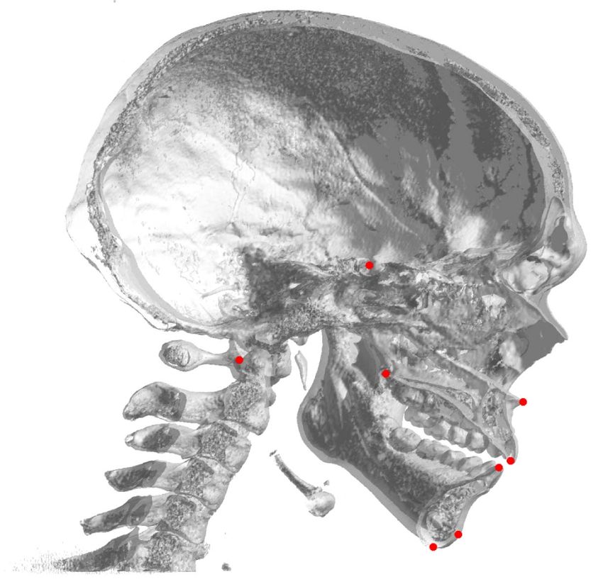
Phys. Med. Biol. 65 (2020) 085018                                                              https://doi.org/10.1088/1361-6560/ab7a71

                           Physics in Medicine & Biology

                           PAPER

                           Learning-based local-to-global landmark annotation for automatic
OPEN ACCESS
                           3D cephalometry
RECEIVED
14 October 2019            Hye Sun Yun1, Tae Jun Jang1, Sung Min Lee1, Sang-Hwy Lee2,3 and Jin Keun Seo1
REVISED                    1
23 February 2020
                               Department of Computational Science and Engineering, Yonsei University, Seoul,
                               Republic of Korea
ACCEPTED FOR PUBLICATION   2
                               Department of Oral and Maxillofacial Surgery, Oral Science Research Center, College of Dentistry, Yonsei University, Seoul,
26 February 2020
                               Republic of Korea
PUBLISHED                  3
                               Author to whom any correspondence should be addressed.
23 April 2020
                           E-mail: sanghwy@yuhs.ac
Original Content from       Keywords: cephalometric landmark, computerized tomography, deep learning
this work may be used
under the terms of the
Creative Commons
Attribution 3.0 licence.
Any further distribution   Abstract
of this work must          The annotation of three-dimensional (3D) cephalometric landmarks in 3D computerized
maintain attribution to
the author(s) and the titletomography (CT) has become an essential part of cephalometric analysis, which is used for
of the work, journal
citation and DOI.          diagnosis, surgical planning, and treatment evaluation. The automation of 3D landmarking with
                           high-precision remains challenging due to the limited availability of training data and the high
                           computational burden. This paper addresses these challenges by proposing a hierarchical
                           deep-learning method consisting of four stages: 1) a basic landmark annotator for 3D skull pose
                           normalization, 2) a deep-learning-based coarse-to-fine landmark annotator on the midsagittal
                           plane, 3) a low-dimensional representation of the total number of landmarks using variational
                           autoencoder (VAE), and 4) a local-to-global landmark annotator. The implementation of the VAE
                           allows two-dimensional-image-based 3D morphological feature learning and
                           similarity/dissimilarity representation learning of the concatenated vectors of cephalometric
                           landmarks. The proposed method achieves an average 3D point-to-point error of 3.63 mm for 93
                           cephalometric landmarks using a small number of training CT datasets. Notably, the VAE captures
                           variations of craniofacial structural characteristics.

                           1. Introduction

                           Cephalometric analysis facilitates the development of morphometrical guidelines for diagnosis, planning,
                           and treatment of craniofacial disease or for evaluations in anthropological research. Recent advances in
                           image processing techniques have allowed the annotation of three-dimensional (3D) cephalometric
                           landmarks in 3D computerized tomography to become an essential clinical task. Cephalometric landmarking
                           is usually performend via manual identification of points that represent craniofacial morphological
                           characteristics. This requires a high level of expertise, time, and labor, even for experts. Therefore, there is an
                           increasing demand for a computer-aided automatic landmarking system that can reduce the
                           labor-intensiveness of this task and improve workflow.
                               Over the past 40 years, several approaches have been proposed for automatic landmark identification
                           based on image processing and pattern recognition (Levy-Mandel et al 1986, Cardillo and Sid-Ahmed 1994,
                           Chakrabartty et al 2003, Giordano et al 2005, Hutton et al 2000, Innes et al 2002, Levy-Mandel et al 1986,
                           Parthasarathy et al 1989, Rudolph et al 1998, Vučinić et al 2010, Codari et al 2017, Gupta et al 2015, Makram
                           and Kamel 2014, Montufar et al 2018). These conventional image processing approaches generally encounter
                           difficulties in achieving robust and accurate landmarking owing to limitations in the simultaneous viewing
                           of local and global geometric cues. Most prior works involved two-dimensional (2D) cephalometry using
                           plain radiographs or CT-derived scan images. However, recent advances in imaging technologies and
                           computer-assisted surgery have facilitated a shift from 2D to 3D cephalometry, which has several advantages
                           over 2D techniques, including accurate identification of anatomical structures, avoidance of geometric

                           © 2020 Institute of Physics and Engineering in Medicine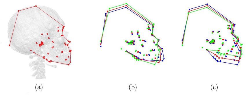
Phys. Med. Biol. 65 (2020) 085018                                                                                       H S Yun et al

distortion in images, and the ability to evaluate complex cranial structures (Lee et al 2014). Most previous 3D
approaches were based on reference models (Codari et al 2017, Makram and Kamel 2014, Montufar et al
2018), and their performance was limited by the unique structural variations of different individuals. This
indicates that there are still limitations in dealing with complex 3D craniofacial model and to formulating it
into well-defined mathematical formulae.
    Recent developments in deep learning for medical imaging applications have led to several attempts to
build an automatic cephalometric landmarking system. The main advantage of these deep learning
approaches compared to conventional image processing is that the experience of the experts can be reflected
in the algorithm through learning training datasets. The architecture for learning datasets labeled by experts
has allowed deep-learning-based methods to locate landmarks in 2D cephalograms with impressive
performance (Arik et al 2017). However, there continue to be difficulties in the application of these methods
to 3D cephalometry because of the required number of datasets. According to Barron’s observation (Barron
1994) regarding approximations with shallow neural networks, the number of training datasets needed for
learning grows tremendously as the input dimensions increase. Due to the high input dimensionality for
cranial CT (typically 512 × 512 × 400 matrix size), much more training datasets are required than are
currently available, especially given the legal and ethical restrictions associated with medical data. Even if a
sufficient amount of data is collected, the learning process can be difficult due to the curse of dimensionality
for processing high dimensional images. These issues represent a significant hindrance to the development of
high-precision, automatic, 3D landmarking systems.
    This paper reports the development and evaluation of an automatic annotation system for 3D
cephalometry using limited training datasets. To address the dimensionality issue and limited data
availability, a hierarchical deep learning method is developed which consists of four stages: 1) a basic
landmark annotator for 3D skull pose normalization, 2) a deep learning-based coarse-to-fine landmark
annotator on the midsagittal plane, 3) a low-dimensional representation of the total number of landmarks
using variational autoencoder (VAE), and 4) a local-to-global landmark annotator. The first stage employs a
shadowed 2D-image-based annotation method (Lee et al 2019) to detect seven basic landmarks, which are
then used for 3D skull pose normalization via rigid transformation and scaling. In the second stage, we
generate partially integrated 2D image on midsagittal plane. By applying a convolutional neural
network-based landmark annotator, the system then roughly estimates the landmarks on 2D image. A
patch-based landmark annotator then provides more accurate detection of the landmarks. Stage 3 applies the
VAE to the affine normalized training datasets (obtained in stage 1) to extract a disentangled
low-dimensional representation. This low-dimensional representation is then used for mapping from
fractional information of the landmarks (obtained in stages 1 and 2) to total information of the landmarks.
An additional benefit of using the VAE is that it can learn variations of craniofacial structural characteristics.
    In this paper, the proposed method was evaluated by comparing the positional discrepancy between the
results obtained and that of the experts. Using a small number of training CT datasets, the proposed method
achieved an average 3D point-to-point error of 3.63 mm for 93 cephalometric landmarks. Therefore, the
proposed method has an acceptable point-to-point error for assisting medical practice.

2. Method

Let x represents a three-dimensional CT image with voxel grid Ω := {v = (v1 , v2 , v3 ) : vj = 1, · · · , dj ,
j = 1, 2, 3} with dj being the number of voxels in direction vj . In our case, the CT image size is approximately
512 × 512 × 400. The value x(v) at the voxel position v can be viewed as the attenuation coefficient. The goal
is to find a map f from the 3D CT     ( image x to )a group of 93 landmarks P (see table A1), where
P = ( p1 , · · · , p93 ) and each pj = pj,1 , pj,2 , pj,3 denotes the 3D position of the jth landmark. P can be
expressed as follows :

                            P = (( p1,1 , p1,2 , p1,3 ), ( p2,1 , p2,2 , p2,3 ), · · · , ( p93,1 , p93,2 , p93,3 )) .            (1)

    The group of landmarks P can be viewed as a geometric feature vector that describes craniofacial skeletal
morphology. Since direct automatic detection of P seems to be quite challenging, it is desirable to infer P
based on minimal information, which is more convenient for automatic detection. By exploiting the
similarity of facial morphology, it is reasonable to have a low dimensional latent representation for feature
vectors. This could be achieved provided that the geometric feature vector can be expressed as a low
dimensional representation, which retains crucial morphological features that describe dissimilarities
between the data. Each step of the proposed method is illustrated in the following subsections (also see
figure 1).

                                                         2
Phys. Med. Biol. 65 (2020) 085018 H S Yun et al
v2
v1 Training low-dimensional representation
v3 VAE
Training Data
x • Normalized landmarks µ
(i)
{P : 1, · · · , N } h
Binarization
Multiple shadowed • Mid-plane landmarks
2D images (i)
{P : 1, · · · , N }
CNN
N
(i)
Γ = argmin N1 Γ(P ) − h(i) 2
Γ i=1
Reference landmarks
Reference coordinate
Image-based Patch-based
v2 v2 CNN CNN
v1
v3 v3
h
Vector Γ Ψ
normalization
xs a b
b
P
Coarse detection Fine detection
a xs (v1 , v2 , v3 )dv1 P
Figure 1. Schematic diagram of the proposed method for the 3D landmark annotation system. The input 3D image x is
standardized/normalized using five reference landmarks in such that the reference landmarks of the corresponding normalized
image x♮ are fixed (to some extent) regardless of the input images. The total group of landmarks P is then detected by combining
two different deep learning methods described in sections 2.2 and 2.3.
Coordinate change
& Rescaling
x x
(a) (b)
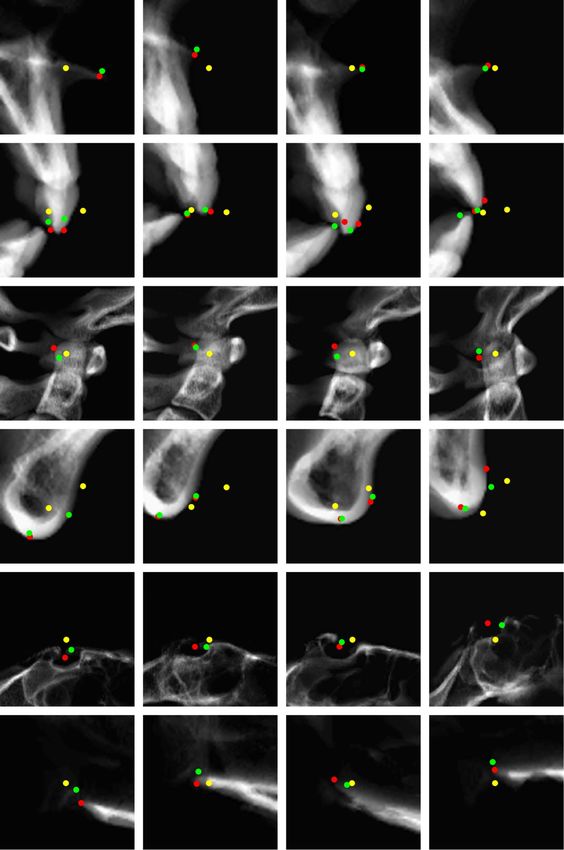
Figure 2. 3D skull pose normalization. (a) The reference hexahedron formed by connecting the five reference landmark points.
(b) The normalization of data by changing the coordinate from machine dependent coordinate to a new coordinate determined
by (a) and by rescaling.
2.1. Stage 1: Choice of a reference coordinate frame and anisotropic scaling for skull normalization
The first step determines a reference coordinate frame and normalizes the data for effective feature learning.
As shown in figure 2, the hexahedron made by the five landmarks (bregma, center of foramen magnum
(CFM), nasion, left/right porion (L/R Po)) is normalized using a suitable anisotropic scaling. The
normalization of the data is based on facial width (the distance between the x-coordinate of L Po and R Po),
facial depth (the distance between y-coordinate of L Po and nasion), and facial height (the distance between
z-coordinate of CFM and bregma). We normalize the data by setting the width, depth, and height as a fixed
value so that each reference hexahedron has (to some extent) fixed shape and size. The hexahedron
determined by geometrical transformation is not exactly in the same size since the landmark positions vary
for different individuals. These reference landmarks can be automatically obtained using the existing
approach of multiple shadowed 2D-image-based landmarking (Lee et al 2019), which utilizes multiple
shadowed 2D images with various lighting and view directions to capture 3D geometric cues. The five
reference landmarks are important components for the normalization of the skull. Also, they are chosen
because they have apparent positional features which enable easy and robust detection even with a small
number of data. The reference coordinate frame is selected so that the CFM is positioned at the origin and
the bregma lies on the z-axis. The midsagittal plane is the yz-plane (x = 0) and is determined by three
landmarks (CFM, bregma, and nasion). We denote x♮ as the CT data with the new reference Cartesian
coordinate. This normalization focuses on facial deformities (e.g. prognathic/retrognathic jaw deformities)
by minimizing scale and pose dependencies, and it enables efficient feature learning of
similarity/dissimilarity in the third stage when applying VAE.
3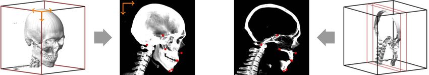
Phys. Med. Biol. 65 (2020) 085018                                                                                          H S Yun et al

                                                                         S

                                                           Od                 PNS
                                                                                           ANS

                                                                                           MxDML
                                                                                         MnDML

                                                                        Me(anat)     Pog

   Figure 3. Landmarks near the midsagittal plane. These landmarks are identified by using coarse-to-fine CNN. The detail for each
   landmark is shown in table A2.

                        Full integration                                                Partial integration
                                              v2
         v2        v1                    v3
              v3
                                                                  vs.

   Figure 4. Fully integrated image vs partially integrated image. A partially projected image is advantageous compared to fully
   projected image in detecting landmarks.

2.2. Stage 2: Detecting landmarks near the midsagittal plane
This step measures 8 landmarks near the midsagittal plane (see figure 3) that are used to estimate the total
landmarks of the skull. Given that the method only considers landmarks that are on or near the midsagittal
plane, not the entire skull, this stage uses a digitally reconstructed 2D image obtained by incorporating
cross-sectional CT images taken near the midsagittal plane (i.e. via integration of truncated binary 3D skull
data). The resulting 2D midsagittal image has less blurring and less irrelevant information (which is caused
by overlapping contralateral structures) than a 2D cephalogram with whole-volume data. Given that
landmarks are determined from the skeletal morphology, image enhancement is used to emphasize bone, as
shown in figure 4. This emphasis on relevant locations helps the machine learning to focus on key
information more efficiently and should improve feature learning despite the limited training datasets.
Enhancement is performed via binarization of the brightness and contrast (setting bone as 1 and other areas
as 0), which allows the machine to discriminate between the necessary and unnecessary image features.
     The 3D CT data are first binarized by thresholding. The truncated volume is then integrated along the
normal direction of the midsagittal plane. The image generated by this method, although 2D, contains 3D
features near the midsagittal plane.
     Let xs be the 3D binary data with the v1 -direction as normal direction of midsagittal plane. The data
xs (v) is given by 1 if x(v) > ζ and 0 otherwise, where ζ is attenuation coefficient of bone. The 2D image
xmid (v2 , v3 ) is obtained by
                                                           ˆ b
                                         xmid (v2 , v3 ) =     xs (v1 , v2 , v3 )dv1 ,                      (2)
                                                                  a

where v1 -directional interval [a, b] determines the truncated volume, as shown in figure 4.
   Let Ploc = (v2,1 , v3,1 , · · · , v2,8 , v3,8 ) denote 8 landmarks on the 2D image. With the dataset
   (i)    (i)
{(xmid , Ploc ) | i = 1, 2, ..., N}, we train a network that detects 8 landmarks on a 2D image using convolutional
neural network (CNN). However, accurate detection of the landmarks directly from image is limited due to
small number of data we have. To address this problem, we use coarse-to-fine detection approach using

                                                       4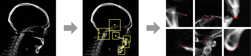
Phys. Med. Biol. 65 (2020) 085018                                                                                      H S Yun et al

                                                                                              ANS
                                                                                                           S        MnDML

                                                                                                                         MxDML

                                                                                                         Od

                                                                                           PNS

                                                                                                                             Pog
                                                                                                                     Me(Anat)

              xmid                            Coarse CNN Detection                        Patch-based Fine CNN Detection
   Figure 5. Coarse-to-fine detection using entire image-based and patch-based CNN. 8 landmarks are roughly detected using the
   entire image-based CNN (coarse detection). Then, patch-based CNN (fine detection) is used to detect each landmark on the
   corresponding local patch obtained from the output of the entire image-based CNN.

                                                     Variational Autoencoder

                                                            μ

                                                                      h
                                                            σ

                normalized landmarks

                                                     Φ                           Ψ
   Figure 6. Architecture of VAE-based low dimensional representation. VAE aims to generate highly reduced encoded vector
   h ∈ R25 which will be decoded to a vector as close to input vector P ∈ R279 . Normalized landmarks are used to generate
   semantically useful latent space.

entire image-based CNN and patch-based CNN. The architectures of CNNs will be explained in result
section. The entire image-based CNN allows to detect Ploc roughly by capturing global information. This
coarse detection output is used to generate local patches, which are input of the patch-based CNN. The
patch-based CNN provides Ploc with improved accuracy. See figure 5.

2.3. Stage 3: Learning a low-dimensional latent representation of landmarks
In this stage, a low-dimensional latent representation of the total landmark vector P is obtained by applying
the VAE (Kingma et al 2013) to the normalized data in stage 1. The change of the coordinates and data
normalization in stage 1 are expected to minimize the scale and pose dependency, allowing more efficient
identification of factors on the midsagittal plane related to facial deformity. This facilitates the extraction of
exploitable morphological factors.
    In mathematical terms, the VAE is a deep learning technique that finds a non-linear expression of the
concatenated landmark vector P ∈ Rk by variables h ∈ Rd (d ≪ k) in the low-dimensional latent space. In
our experiments, we use k = 279 and d = 25. The VAE uses the training datasets {P(i) : i = 1, · · · , N} to learn
two functions, the encoder Φ : P → h and the decoder Ψ : h → P using the following loss minimization over
the training data:

                                 1 ∑[                                                            ]
                                   N
               (Ψ, Φ) = argmin        ∥Ψ ◦ Φ(P(i) ) − P(i) ∥2 + DKL (N (µ(i) , Σ(i) ) ∥ N (0, I)) ,                                (3)
                       (Ψ,Φ)∈VAE N         i=1

where VAE describes a class of functions in the form of the deep learning network described in figure 6. To
be precise, the encoder Φ is of the following nondeterministic form:

                                                    Φ(P) = µ + σ ⊙ hnoise                                                          (4)

where µ = (µ(1), · · · , µ(d)) ∈ Rd represents a mean vector; σ = (σ(1), · · · , σ(d)) ∈ Rd is a standard
deviation vector; hnoise is an auxiliary noise variable sampled from standard normal distribution N (0, I); and
⊙ is the element-wise product (Hadamard product). Hence, Φ(P) ∼ N (µ, Σ) where Σ is a diagonal

                                                     5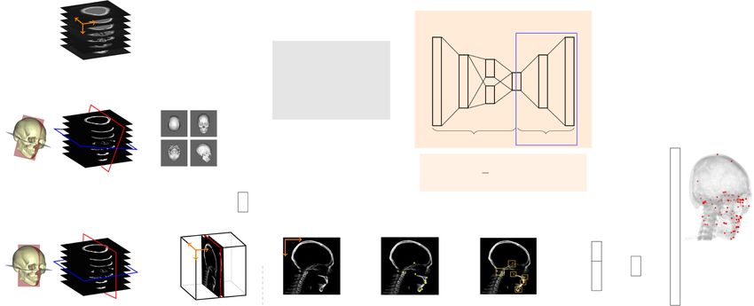
Phys. Med. Biol. 65 (2020) 085018                                                                              H S Yun et al

                                                             Training

                                                   (i)
                                               P                        h(i) =      (P(i) )

                     Reference
                    Landmarks

   Figure 7. Local-to-global landmark annotation Ψ◦ Γ. The map Γ : P♯ → h is trained using the dataset
                       (i )
   {(h(i) = Φ(P(i) ), P♯ ) : i = 1, · · · , N} generated from the encoder Φ in stage 3.

covariance matrix Σ = diag(σ(1)2 , · · · , σ(d)2 ). The term DKL (N (µ(i) , Σ(i) ) ∥ N (0, I)) in (3) denotes the
Kullback-Leibler (KL) divergence between N (µ, Σ) and N (0, I), which is defined by

                                                              1 ∑ [ (i) 2                                 ]
                                                                  d
                    DKL (N (µ(i) , Σ(i) ) ∥ N (0, I)) =            (µ (j) + σ (i) (j)2 − log σ (i) (j) − 1 .            (5)
                                                              2
                                                                 j=1

Note that the covariance Σ and DKL (N (µ, Σ) ∥ N (0, I)) are used for smooth interpolation and compact
encoding.
    The decoder Ψ : h → P in (3) provides a low-dimensional disentanglement representation, so that each
latent variable is sensitive to changes in individual morphological factors, while being relatively insensitive to
other changes. The changes are visualized in discussion section.

2.4. Stage 4: Local-to-global landmark annotation for automatic 3D cephalometry
In this final step, we detect the total landmark vector (P) from the fractional information (P♯ ), where P♯ is
the vector composed of Ploc obtained in stage 2 and the reference landmarks in stage 1. In stage 3, the VAE
can find a low-dimensional latent representation of the total landmarks, i.e. Ψ(h) = P. Stage 2 detects a
portion of the landmarks Ploc near the midsagittal plane. Using the encoder map h(i) = Φ(P(i) ) in the result
                                        (i)
of stage 3, the training data {(h(i) , P♯ ) : i = 1, 2, ..., N} can be generated. Then, the training data can be used
to learn a non-linear map Γ : P♯ → h that connects the latent variables h and the fractional data P♯ . The
                                                                                   ∑N          (i)
non-linear regression map Γ : P♯ → h is obtained by minimizing the loss N1 i=1 ||Γ(P♯ ) − h(i) ||2 . The
local-to-global landmark annotation is then obtained from

                                                             (Ψ ◦ Γ)(P♯ ) = P                                           (6)

This is represented in figure 7.

3. Results

3.1. Dataset and experimental setting
We used two datasets, provided by one of authors. The first dataset contains 26 anonymized CT data with
cephalometric landmarks that were produced for a previous study (Lee et al 2014). Normal Korean adults
with skeletal class I occlusion (10 males and 16 females; 24.22±2.91 years) volunteered for the previous
study, which was approved by the local ethics committee of the Dental College Hospital, Yonsei University,
Seoul, Korea (IRB number: 2-2009-0026). Informed consent was obtained from each subject. This dataset
was used to train convolutional neural network (CNN) for automated 2D landmarking. The size of the
original CT image was 512 × 512 ×(number of slices), where the number of slices varies from 350 to 500. To
make all the input data a uniform size, we resized each image to 512 × 512 × 512 using zero-padding (filling
in the missing parts with zero). The labeling of the landmarks on the CT image was performed via manual

                                                         6
Phys. Med. Biol. 65 (2020) 085018 H S Yun et al
Fully connected, 1024
2 × 2 Conv(stride 2), 128
2 × 2 Conv(stride 2), 128
Fully connected, 512
Fully connected, 256
2 × 2 Conv(stride 2), 16
2 × 2 Conv(stride 2), 32
2 × 2 Conv(stride 2), 64
2 × 2 Conv(stride 2), 8
3 × 3 Conv, 128
3 × 3 Conv, 128
3 × 3 Conv, 128
3 × 3 Conv, 128
3 × 3 Conv, 16
3 × 3 Conv, 16
3 × 3 Conv, 16
3 × 3 Conv, 32
3 × 3 Conv, 32
3 × 3 Conv, 32
3 × 3 Conv, 64
3 × 3 Conv, 64
3 × 3 Conv, 64
3 × 3 Conv, 8
3 × 3 Conv, 8
3 × 3 Conv, 8
Output
Input
(a)
Fully connected, 128
2 × 2 Conv(stride 2), 16
2 × 2 Conv(stride 2), 8
2 × 2 Conv(stride 2), 8
Fully connected, 32
3 × 3 Conv, 16
3 × 3 Conv, 16
3 × 3 Conv, 16
3 × 3 Conv, 8
3 × 3 Conv, 8
3 × 3 Conv, 8
3 × 3 Conv, 8
3 × 3 Conv, 8
3 × 3 Conv, 8
Output
Input
(b)
Figure 8. Architectures of (a) entire image-based CNN and (b) patch-based CNN. The entire image-based CNN allows to detect
Ploc roughly. Then the patch-based CNN provides Ploc with improved accuracy by using local patches generated from the entire
image-based CNN.
marking. The second dataset with 3D positions of landmarks from anonymized 229 subjects with dentofacial
deformity and malocclusion was also used, and they were acquired in excel format using the 3D coordinates
of landmarks from the original data source. The labeling of the landmarks for both datasets was performed
by one author (LSH) with more than 20 years of experience in 3D cephalometry. When training CNN, we
used the first dataset of 22 subjects as training data and four as test data. Translation was applied for data
augmentation. For VAE and non-linear regression, we used both the first dataset (26 subjects) and the
second dataset (229 subjects), having total 255 subjects. We used 230 subjects as training data and 25 as test
data. For each experimental setting, we set learning rate as 0.0001 and batch size as 8, and went through 3000
iterations when training CNN. For VAE and non-linear regression, we set learning rate as 0.0001 and batch
size as 50, and performed 30 000 iterations. Adam (Kingma et al 2014), which is an adaptive gradient
method, was chosen as the optimization algorithm.
3.2. Experimental results
In our proposed method, we aimed to locate 3D coordinates of 93 landmarks from fractional information
consisting of Ploc obtained in stage 2 and the reference landmarks in stage 1.
We normalized the data by changing the coordinate and rescaling the size of the data. To set the new
coordinate system, seven landmarks (CFM, bregma, nasion, left/right porion, and left/right orbitale) were
used. Then, using these landmarks, we applied anisotropic scaling by fixing the height as 145 mm, the width
as 110 mm, and the depth as 80 mm,. These values represented the average value height, width, and depth,
respectively, of the sample. The normalization of the skull was empirically performed based on tables 3 and 4,
which show the variances of landmark positions for three types of scaling methods. The anisotropic scaling
has the smallest variance for landmarks on neurocranium, compared to the other scaling methods.
For the detection of 8 landmarks (see table A2) on the midsagittal plane using truncated 2D image, the
interval for truncation of the 3D data was set at 3 cm (dist(a, b) = 3 cm), v1 -directionally ±1.5 cm from the
midsagittal plane. The overall architecture for image-based CNN is shown in figure 8(a). With the input data
of size 512 × 512, the first three layers were convolutional layers with kernel size of 3 × 3 pixels with stride 1
and 8 channels. On the fourth layer, we used kernel size of 2 × 2 convolution with stride 2 for spatial
downsampling. By applying either convolution or pooling layer to each layer, the last four layers were fully
connected layers with 1024-512-256-16 neurons in each layer. Rectified Linear Unit (ReLU) activation was
performed after each pooling layer to solve vanishing gradient problem, dropout rate of 0.75 was chosen to
alleviate overfitting problem (Srivastava et al 2014), and Adam optimizer was used for learning. Additionally,
we extracted local patch using the output obtained from entire image-based CNN. For fine detection of the 8
landmarks on the midsagittal plane, CNN architecture was again designed for the patch-based detection. The
architecture is similar to that of entire image-based CNN as shown in figure 8(b). Note that the size of the
patch (as input for patch-based CNN) was chosen by the characteristics of morphological structures in the
7Phys. Med. Biol. 65 (2020) 085018 H S Yun et al
ANS
MxDML
MnDML
Od
Pog
Me(Anat)
S
PNS
Figure 9. Results of coarse-to-fine landmark detection on a 2D image. The yellow dot is the output of the entire image-based
CNN, which determines each patch. The green dot is the output for detection using patch-based CNN. The red dot is the ground
truth.
vicinity of the landmarks. With small amount of data at our hands, it was inevitable to apply landmark
detection additionally on the small patches for better feature learning for each landmark. The effectiveness of
additional detection on a small ROI is shown in figure 9, and table 1 shows the prediction error value of the
landmarks. It is observed that detection on the small patch captures more accurate features for each
landmark so that the patch-based CNN output becomes closer to the ground truth compared to the
detection of entire image-based CNN.
As a key aspect of this research, we used VAE to find the latent representation of the landmark feature
vector. The objective was to find the low dimensional representation of high dimensional landmark feature
vectors. The latent dimension of the latent space was empirically chosen to be 25, which indicates that the
landmark feature vectors (∈ R279 ) can be nonlinearly expressed using 25 variables. Next, we connected the
landmarks detected in previous steps to the trained representation via non-linear regression with multilayer
perceptron. The multilayer perceptron structure was set as 45-30-25 neurons in each layer. After the
completion of training VAE and non-linear regression, the reconstructed landmark vectors were given by
(Ψ ◦ Γ)(P♯ ). Let qj denotes the denormalized vector of jth component (jth landmark) of (Ψ ◦ Γ)(P♯ ).
∑N (i) (i)
Figure 10 shows the 3D distance error (mm) for each landmark, which is calculated as N1 i=1 ∥qj − pj ∥,
(i) (i)
where ∥qj − pj ∥ indicates the error for ith patient. The localization errors of most of the landmarks were
within 4 mm. We achieved an average point-to-point error of 3.63 mm for 93 cephalometric landmarks
8Phys. Med. Biol. 65 (2020) 085018 H S Yun et al
Table 1. Mean of 2D distance error (mm) for 8 landmark detection using coarse-to-fine annotator on test data. Each column indicates
the errors of the coarse detection and the fine detection respectively.
Landmark Coarse detection error (mm) Fine detection error (mm)
ANS 3.97 0.88
Me(anat) 5.84 0.62
MnDML 3.23 1.45
MxDML 3.46 1.39
Od 6.12 2.73
PNS 3.81 2.63
Pog 5.67 1.51
S 6.13 3.75
(mm) Mean error : 3.63mm
8
7
localization errors
6
Landmark
5
4
3
2
1
0 10 20 30 40 50 60 70 80 90
Cephalometric landmarks
Figure 10. The landmark localization errors (mm) for 93 cephalometric landmarks for the test dataset. Red dots denote the 3D
distance error for each landmark, and the blue line represents the average point-to-point error for 93 landmarks (3.63 mm).
∑93 1 ∑N (i) (i)
i=1 ∥qj − pj ∥). The standard deviation of the error of the 93
1
which was calculated by 93 j=1 ( N
landmarks was 1.41 mm. The landmark point for midpoint of superior pterygoid point (mid-Pts) exhibited
the highest level of accuracy with an error of 1.41 mm for a 3D distance, and the point for right coronoid
point (R COR) exhibited the lowest level of accuracy with an error of 7.47 mm for a 3D distance. For the
total number of points, the error was within 8 mm and 60 landmarks were within 4 mm. Figure 10 shows the
test error for each landmark.
4. Discussion
4.1. About usage of CT data
3D cephalometry serves as a powerful tool in craniofacial analysis, as compared to 2D cephalometry (Adams
et al 2004, Nalçaci et al 2010). It is based on 3D CT images obtained from conebeam CT (CBCT) or
multi-slice CT (MSCT). The effective dose for CBCT in craniofacial imaging is generally lower than that of
MSCT (Ludlow et al 2013). Since our currently available CBCT machines do not provide the full field of view
for complete 3D cephalometric analysis such as Delaire or Sassouni analysis, we applied our experiments to
previously acquired MSCT images that contain cranium and vertebrae as well as the maxillomandibular
facial structures. Low dose and radiation protection protocol for MSCT were applied to reduce the radiation
dose during the study.
4.2. About the number of cephalometric landmarks
For general 2D cephalometric analysis, 93 landmarks can be considered to be too many. However, such
number of landmarks are needed for realization and clinical application of 3D cephalometry. Among the 93
landmarks, 75 points were consisted of bilateral reference points (29 landmarks respectively for left and
right) and their middle points (17 midpoints of left and right). Therefore, it matched with 47 landmarks
(18 midline and 29 bilateral points) for 2D cephalometry. Due to the characteristics of the 3D analysis, the
midpoints are needed to construct their related planes. Without the midpoints, some complicated problems
can be expected. For example, the reference planes created only with bilateral landmarks may not have a
9Phys. Med. Biol. 65 (2020) 085018 H S Yun et al
Table 2. Comparison of errors of VAE-based expression for P by varying latent dimension. In this case, the error is the difference
1 ∑N
between the input and output that is given as ∥Ψ ◦ Φ(P(i) ) − P(i) ∥2 in section 2.3. The proposed method is highlighted, where
N i=1
1.98 (3.25) indicates a mean error of 1.98 and a maximum error of 3.25 for training data.
Latent No normalization (mm) Rotation only (mm) Rotation + Rescaling (mm)
dimension Train Test Train Test Train Test
10 4.37 (8.58) 6.37 (14.67) 2.52 (4.63) 3.59 (5.27) 2.87 (5.33) 3.16 (3.90)
15 4.49 (8.72) 6.67 (11.91) 2.16 (3.79) 3.26 (7.49) 2.37 (4.22) 2.89 (3.54)
20 4.11 (8.34) 6.63 (13.88) 1.99 (3.31) 2.89 (4.72) 2.41 (4.53) 2.83 (3.55)
25 4.29 (8.43) 5.20 (9.27) 1.96 (3.21) 2.98 (5.77) 1.98 (3.25) 2.54 (3.26)
30 4.09 (8.69) 5.95 (13.52) 2.21 (3.38) 2.84 (3.88) 2.17 (3.60) 3.06 (6.89)
Table 3. Variances of landmarks on the neurocranium for three types of scaling methods. The anisotropic scaling shows the lowest
variance for most neurocranium landmarks among three scaling methods.
Landmark L Clp LM L Or L Po Na Od R Clp RM R Or R Po SC
No scaling (mm) 3.63 6.74 7.16 6.00 6.79 4.54 3.54 6.68 7.30 5.97 8.24
Anisotropic
(mm) 3.07 5.87 7.38 4.95 5.70 4.76 3.00 5.74 7.23 4.39 8.02
Isotropic (mm) 5.35 6.08 6.77 5.93 6.14 4.61 5.30 6.07 7.03 5.88 6.80
Table 4. Variances of landmarks on the mandible for three types of scaling methods. The anisotropic scaling shows the highest variance
for most mandible landmarks among three scaling methods. Hence, the proposed anisotropic scaling approach allows morphological
differences of the mandible to be emphasized.
Landmark LF RF L-Go mid R-Go mid Me(anat) Pog
No scaling (mm) 8.64 8.35 10.19 10.50 16.10 16.01
Anisotropic (mm) 9.38 8.84 10.64 10.78 16.72 16.56
Isotropic (mm) 8.76 8.40 10.07 10.38 16.26 16.14
Table 5. Average 3D distance of point-to-point error (mm) of 93 landmarks for the choice of local landmarks. The table shows the mean
value, standard deviation and the maximum value.
Choice of landmarks Train (mm) Test (mm)
11 landmarks
(midsagittal plane) 4.23 ± 0.90 (8.66) 4.32 ± 0.98 (7.77)
15 landmarks
(our proposed method) 3.86 ± 0.85 (8.94) 3.95 ± 0.64 (5.07)
27 landmarks
(neurocranium + midsagittal plane) 3.53 ± 1.55 (10.22) 3.26 ± 0.71 (5.96)
vertical relationship with the midsagittal plane, which causes inconsistent cephalometric measurements.
Therefore, as compared to 2D analysis, 3D cephalometrics require nearly three times more landmarks for
cephalometric measurement, since bilateral landmarks are considered to be unilateral in 2D cephalometric
analysis.
4.3. About data normalization
In the initial step of our proposed method, we set a new coordinate system (rotation and rescaling) for data
normalization. Table 2 shows the average 3D distance error for a total of 93 landmarks by varying the latent
dimension and the normalization scheme. In this case, the error is the difference between the input and
1 ∑N
output that is given by ∥Ψ ◦ Φ(P(i) ) − P(i) ∥2 (see equation (3) in section 2.3). Based on a
N i=1
comparison of the errors of the VAE-based expression for P for various latent dimensions, we empirically
chose the latent dimension to be 25 for the normalized data, which shows the lowest mean and maximum
error for the test dataset.
To evaluate the scaling methods, we measured the variance of each landmark position between subjects
with CFMs that are fixed as the origin. Tables 3 and 4 show the variances of landmark positions for three
types of scaling methods (no scaling, isotropic scaling, and anisotropic scaling). Each of the table refers to the
landmarks of the neurocranium and mandible, respectively.
10Phys. Med. Biol. 65 (2020) 085018 H S Yun et al
Figure 11. Variations of craniofacial structural characteristics. (a) is the landmark Ψ(Φ(P)) on the corresponding image. Two
observable factors are shown in (b) and (c). (b) shows that latent variable corresponds to prognathic and retrognathic movement,
(c) represents the change of facial height. The green, red and the blue points are reconstructed data Ψ(Φ(P) − 10ej ), Ψ(Φ(P)),
and Ψ(Φ(P) + 10ej ) respectively where ej is a unit vector with jth component is one and otherwise zero.
(1 − t)h(i) + th(j) for 0 < t < 1
h(i) h(j)
Figure 12. Interpolation between two points h(i) and h( j) in the latent space. Given two feature vectors Ψ(h(i) ) and Ψ(h( j) ),
VAE allows to generate the interpolated feature vector Ψ((1 − t)h(i) + th( j) ) for 0 < t < 1.
4.4. About choice of local landmarks
In stage 4, we detect the 93 global landmarks from 15 local landmarks, some of which are on the surface of
the skull and the others lie on the midsagittal plane. Table 5 shows the average 3D distance of point-to-point
error for the 93 landmarks, for the selection of local landmarks. It is expected that a higher level accuracy will
be obtained for cephalometric annotation if there are more (quantitative) local landmarks. To further detect
local landmarks such as those on the surface of the skull (e.g. neurocranium landmarks), it would be possible
to detect landmarks using an existing method based on multi-shaded 2D image-based landmarking (Lee et al
2019). Therefore, the proposed method could be improved by detecting more local landmarks.
4.5. About variations of craniofacial structural characteristics
The results of experiments using the VAE show that the geometric feature vector that describes facial skeletal
morphology lies on a low-dimensional latent space. Regarding what each latent variable represents, we
visualized that varying each variable alters the landmark positions. Among 25 latent variables, figure 11
shows visualization of two factors with the changed positions of reconstructed landmarks. Each of them
seems to capture prognathic/retrognathic jaw deformity (figure 11(b)) and the long/short face (by changed
facial vertical dimension) (figure 11(c)). Since these deformity shifts can be regarded as one illustration of
jaw deformity types based on the shape, size, and position of mandible and maxilla, it is interesting that VAE
captures the variations of some craniofacial structure. In this work, we described only two morphological
11Phys. Med. Biol. 65 (2020) 085018 H S Yun et al
factors. We expect that facial deformities would be expressed into the latent variables. Further research is
necessary to deal with it through factor analysis using VAE.
Moreover, to verify one of the properties of VAE i.e. that the latent space is dense and smooth, figure 12
shows the interpolation between two randomly chosen data points in the latent space. We interpolated two
encoded data (say h(i) and h( j) ) and decoded the interpolated samples back to the original space (landmark
data space). Let P(i) , P( j) be data from the landmark data space and h(i) = Φ(P(i) ), h( j) = Φ(P( j) ) be the
encoded data on the latent space. We linearly interpolated two latent vectors and fed them to decoder.
Figure 12 shows the visualization of the decoded data. It can be observed that each of the generated images
contains human-like cephalometric structure landmarks.
5. Conclusion
In this paper, a multi-stage deep learning framework is proposed for automatic 3D cephalometric landmark
annotation. The proposed method initially detects a few landmarks (7 out of 93) that can be robustly and
accurately estimated from the skull image. The knowledge of the 7 landmarks allows the midsagittal plane to
be determined, on which 8 important landmarks lie. This midsagittal plane is used to accurately estimate the
8 landmarks based on the coarse-to-fine CNN in stage 2. The remainder of the landmarks (78 = 93 − 15) are
estimated from the knowledge of 15 landmarks and the VAE-based representation of morphological
similarity/dissimilarity of the normalized skull. This mimics the detection procedure of experts in that it first
estimates easily detectable landmarks, and then detects the remainder of the landmarks. Its novel
contribution is the use of a VAE for 2D image-based 3D feature learning by representing high-dimensional
3D landmark feature vectors using much lower-dimensional latent variables. This low-dimensional latent
representation is achieved with the help of cranial normalization and fixed reference Cartesian coordinates. It
allows all 3D landmarks to be annotated from partial information based on landmarking on a cross-sectional
CT image of the midsagittal plane. The experiments confirmed the capability of the proposed method, even
when a limited number of training datasets were used. Manual landmarking of nearly a hundred of
landmarks is time-consuming and labor-intensive work. Compared to the manual operation, automatic
landmark detection with additional fine tuning is expected to improve the work efficiency of experts.
Therefore, the proposed method has potential to alleviate experts’ time-consuming workflow by dramatically
reducing the time required for landmarking while preserving high accuracy.
Our hierarchical method exhibited a much higher level of performance compared to the previous 3D
deep learning method (Kang et al 2019). Using the same dataset, the proposed method yielded an average 3D
distance error of 3.63 mm for 93 cephalometric landmarks, while the 3D deep learning model (Kang et al
2019) resulted in an average 3D distance error of 7.61 mm only for 12 cephalometric landmarks.
The proposed method exhibited relatively high performance, but the error level did not meet the
requirement for immediate clinical application (such as in less than 2 mm of error levels). However this
approach has a lot of room for improvement and the errors can be significantly reduced by improving deep
learning performance with an increased number of training data. Although our protocol cannot intuitively
determine the exact location set to achieve the expert human standards, it can immediately help guide the
operator to the approximate position and image setting for 3D cephalometry. It can also reduce the burden
of moving the 3D skull object and scrolling over the multi-planar image settings during landmark pointing
tasks. Finally, it can be applied prior to data processing for segmentation, thus assisting in the orientation of
the head to the calibrated posture.
The proposed multi-stage learning framework is designed to deal with the challenge of a small amount of
data when learning 3D features from 3D CT data. Although hospitals generate many CT datasets, few
datasets can be used for research for legal and ethical reasons.
This automatic 3D cephalometric annotation system is in an early stage of development, and there is
potential for further improvement. The proposed method can provide excellent initial landmark estimation
(that only requires small adjustments) that can be used to develop an accurate and consistent landmark
detection system without using a large amount of data. More precisely, with given initial landmark
estimation, the landmark detection problem can be reduced to adjusting the landmark position in each small
region extracted from the initial landmarks. We think that the desired level of accuracy can be achieved if
more data is available. Since the dimension of the input (extracted small region) is small, we do not need
much more training data for better result. Also, it would be desirable to integrate the multi-stage hierarchical
learning framework used in this study with a unified learning framework, because the errors in each step can
affect the successive steps in the hierarchical structure.
12Phys. Med. Biol. 65 (2020) 085018 H S Yun et al
Acknowledgments
This work was supported by the National Research Foundation of Korea (NRF) grant 2015R1A5A1009350
and 2017R1A2B20005661.
Appendix A. Cephalometric landmarks
Table A1. Total 93 cephalometric landmarks consisting landmark feature vector P.
Index Landmark
1 ♯16 tip (The mesiobuccal cusp tip of maxillary right first molar)
2 ♯26 tip (The mesiobuccal cusp tip of maxillary left first molar
3 ♯36 tip (The mesiobuccal cusp tip of mandibular left first molar)
4 ♯46 tip (The mesiobuccal cusp tip of mandibular right first molar)
5 ANS (Anterior nasal spine)
6 ANS’ (Constructed ANS point)
7 AO (Anterior occlusal point)
8 Bregma
9 CFM (Center of foramen magnum)
10 FC (Falx cerebri)
11 L CON (Left condylar point)
12 L COR (Left coronoid point)
13 L Clp (Left posterior clinoid process)
14 L Cp (Left posterior condylar point)
15 L Ct-in (Left medial temporal condylar point)
16 L Ct-mid (midpoint between left Ct-in and Ct-out)
17 L Ct-out (Left lateral temporal condylar point)
18 L EC (Left eyeball center)
19 L F (Left mandibular foramen)
20 L FM (Left frontomaxillary suture)
21 L Go-inf (Left inferior gonion point)
22 L Go-mid (midpoint between the posterior and inferior gonion point)
23 L Go-post (Posterior gonion point)
24 L Hyp (Left hypomochlion)
25 L L1 apex (Root apex of left mandibular central incisor)
26 L L1 tip (Incial tip midpoint of left mandibular central incisor)
27 L LCP (Left lateral condylar point)
28 L M (Left junction of nasofrontal, maxillofrontal, and maxillonasal sutures)
29 L MCP (Left medial condylar point)
30 L MF (Left mental foramen)
31 L NP (Left nasopalatine foramen)
32 L Or (Left orbitale)
33 L Po (Left porion)
34 L Pti (Left inferior pterygoid point)
35 L Pts (Left superior pterygoid point)
36 L U1 apex (Left upper incisal apex)
37 L U1 tip (Left upper incisal tip)
38 L a-Go notch (Left antegonial notch)
39 L mid-F MF (Midpoint between left mandibular foramen and mental foramen)
40 Me(anat) (Anatomical menton)
41 MnDML (Mandibular dental midline)
42 MxDML (Maxillary dental midline)
43 Nasion
44 Od (Odontoid process)
45 PNS (Posterior nasal spine)
46 Pog (Pogonion)
47 R CON (Right condylar point)
48 R COR (Right coronoid point)
49 R Clp (Right posterior clinoid process)
50 R Cp (Right posterior condylar point)
51 R Ct-in (Right medial temporal condylar point)
13Phys. Med. Biol. 65 (2020) 085018 H S Yun et al
Table A1. (Continued)
52 R Ct-mid (midpoint between right Ct-in and Ct-out)
53 R Ct-out (Right lateral temporal condylar point)
54 R EC (Right eyeball center)
55 R F (Right mandibular foramen)
56 R FM (Right frontomaxillary suture)
57 R Go-inf (Right inferior gonion point)
58 R Go-mid (midpoint between the posterior and inferior gonion point)
59 R Go-post (Posterior gonion point)
60 R Hyp (Right hypomochlion)
61 R L1 apex (Root apex of left mandibular central incisor)
62 R L1 tip (Incial tip midpoint of left mandibular central incisor)
63 R LCP (Right lateral condylar point)
64 R M (Right junction of nasofrontal, maxillofrontal, and maxillonasal sutures)
65 R MCP (Right medial condylar point)
66 R MF (Right mental foramen)
67 R NP (Right nasopalatine foramen)
68 R Or (Right orbitale)
69 R Po (Right porion)
70 R Pti (Right inferior pterygoid point)
71 R Pts (Right superior pterygoid point)
72 R U1 apex (Right upper incisal apex)
73 R U1 tip (Left upper incisal tip)
74 R a-Go notch (Right antegonial notch)
75 R mid-F MF (Midpoint between right mandibular foramen and mental foramen)
76 SC (Summit of cranium)
77 mid (Oi -mid-M) (Midpoint between inferior occipital point and mid right-left M point)
78 mid-Clp (mid point between right and left posterior clinoid point)
79 mid-Cp (midpoint between right and left posterior condylar point)
80 mid-Ct (midpoint between R Ct-mid and L Ct-mid)
81 mid-EC (midpoint between R EC and L EC)
82 mid-F (midpoint between R F and L F)
83 mid-FM (midpoint between R FM and L FM)
84 mid-L1 tip (midpoint between right and left lower incisor tip point)
85 mid-M (midpoint between R M and L M)
86 mid-MF (midpoint between R MF and L MF)
87 mid-NP (midpoint between R NP and L NP)
88 mid-Or (midpoint between R Or and L Or)
89 mid-Po (midpoint between R Po and L Po)
90 mid-Pti (midpoint between R Pti and L Pti)
91 mid-Pts (midpoint between R Pts and L Pts)
92 mid-U1 tip (midpoint between right and left upper incisor tip point)
93 midpoint of R-L mid-F MF (midpoint between R mid-F MF and L mid-F MF)
Table A2. Definitions of 15 cephalometric landmarks consisting P♯ . The first eight landmarks are the ones on midsagittal plane.
The others are the reference landmarks.
Landmark Definition Bilaterality
ANS Most anterior point on maxillary bone
Me(anat) Most inferior point along curvature of chin
MnDML Mandibular dental midline
MxDML Maxillary dental midline
Od Highest point on the slope of second vertebra at the point tangent to the line
from posterior clinoid process at the midsagittal plane
PNS Posterior limit of bony palate or maxilla
Pog Most anterior point of mandibular symphysis
S Point representing the midpoint of the pituitary fossa
Bregma Intersection of sagittal and coronal sutures
joining the parietal and frontal bones come together
CFM Center of foramen magnum at the level of basion
Nasion Most anterior point on frontonasal suture of the midsagittal plane
Porion Most superior point of outline of external auditory meatus Yes
Orbitale Most inferior point on margin of orbit Yes
14Phys. Med. Biol. 65 (2020) 085018 H S Yun et al
References
Adams G L, Gansky S A, Miller A J, Harrell Jr W E and Hatcher D C 2004 Comparison between traditional 2-dimensional cephalometry
and a 3-dimensional approach on human dry skulls Am. J. Orthod. Dentofacial. Orthop. 126 397–409
Arik S Ö, Ibragimov B and Xing L 2017 Fully automated quantitative cephalometry using convolutional neural networks J. Med. Imaging
4 014501
Barron A R 1994 Approximation and estimation bounds for artificial neural networks Mach. Learn. 14 115–133
Cardillo J and Sid-Ahmed M A 1994 An image processing system for locating craniofacial landmarks IEEE Trans. Med. Imaging
13 275–289
Chakrabartty S, Yagi M, Shibata T and Cauwenberghs G 2003 Robust cephalometric landmark identification using support vector
machines Multimedia and Expo, 2003. ICME’03. Proc. 2003 Int. Conf. on Multimedia and Expo 3 429–32
Codari M, Caffini M, Tartaglia G M, Sforza C and Baselli G 2017 Computer-aided cephalometric landmark annotation for CBCT data
Int. J. Comput. Assist. Radiol. Surg. 12 113–121
Giordano D, Leonardi R, Maiorana F, Cristaldi G and Distefano M L 2005 Automatic landmarking of cephalograms by cellular neural
networks Conf. on Artificial Intelligence in Medicine in Europe (Berlin: Springer) vol 3 pp 333–342
Gupta A, Kharbanda O P, Sardana V, Balachandran R and Sardana H K 2015 A knowledge-based algorithm for automatic detection of
cephalometric landmarks on CBCT images Int. J. Comput. Assist. Radiol. Surg. 10 1737–1752
Hutton T J, Cunningham S and Hammond P 2000 An evaluation of active shape models for the automatic identification of
cephalometric landmarks Eur. J. Orthod. 22 499–508
Innes A, Ciesielski V, Mamutil J and John S 2002 Landmark detection for cephalometric radiology images using pulse coupled neural
networks Proc. Int. Conf. on Artificial Intelligence IC-AI ’02 (Las Vegas, NV, 24–27 June 2002) vol 2
Kang S H, Jeon K, Kim H, Seo J K and Lee S 2019 Automatic three-dimensional cephalometric annotation system using
three-dimensional convolutional neural networks: a developmental trial Comput. Methods Biomech. Biomed. Eng. Imaging Vis.
8 210–8
Kingma D P and Ba J 2014 Adam: A method for stochastic optimization arXiv: 1412.6980
Kingma D P and Welling M 2013 Auto-encoding variational Bayes arXiv: 1312.6114
Lee S-H, Kil T-J, Park K-R, Kim B C, Piao Z and Corre P 2014 Three-dimensional architectural and structural analysis-a transition in
concept and design from Delaire’s cephalometric analysis Int. J. Oral. Maxillofac. Surg. 43 1154–1160
Lee S M, Kim H P, Jeon K, Lee S H and Seo J K 2020 Automatic 3D cephalometric annotation system using shadowed 2D image-based
machine learning Phys. Med. Biol. 64 055002
Levy-Mandel A, Venetsanopoulos A and Tsotsos J 1986 Knowledge-based landmarking of cephalograms Comput. Biomed. Res.
19 282–309
Ludlow J B and Walker C 2013 Assessment of phantom dosimetry and image quality of i-CAT FLX cone-beam computed tomography
Am. J. Orthod. Dentofacial. Orthop. 144 802–817
Makram M and Kamel H 2014 Reeb graph for automatic 3D cephalometry IJIP 8 17–29
Montufar J, Romero M and Scougall-Vilchis R J 2018 Automatic 3-dimensional cephalometric landmarking based on active shape
models in related projections Am. J. Orthod. Dentofacial. Orthop. 153 449–458
Nalçaci R, Öztürk F and Sökücü O 2010 A comparison of two-dimensional radiography and three-dimensional computed tomography
in angular cephalometric measurements Dentomaxillofac. Radiol. 39 100–106
Parthasarathy S, Nugent S, Gregson P and Fay D 1989 Automatic landmarking of cephalograms Comput. Biomed. Res 22 248–269
Rudolph D, Sinclair P and Coggins J 1998 Automatic computerized radiographic identification of cephalometric landmarks Am. J.
Orthod. Dentofacial. Orthop. 113 173–179
Srivastava N, Hinton G, Krizhevsky A, Sutskever I and Salakhutdinov R 2014 Dropout: a simple way to prevent neural networks from
overfitting J. Mach. Learn. Res. 15 1929–1958
Vučinić P, Trpovski ź and Žćepan I 2010 Automatic landmarking of cephalograms using active appearance models Eur. J. Orthod.
32 233–241
15You can also read