Evaluation of Antarctic Ozone Profiles derived from OMPS LP by using Balloon borne Ozonesondes
←
→
Page content transcription
If your browser does not render page correctly, please read the page content below
www.nature.com/scientificreports
OPEN Evaluation of Antarctic Ozone
Profiles derived from OMPS‑LP
by using Balloon‑borne
Ozonesondes
Edgardo Sepúlveda1, Raul R. Cordero1*, Alessandro Damiani2, Sarah Feron1,3*,
Jaime Pizarro1, Felix Zamorano4, Rigel Kivi5, Ricardo Sánchez6, Margarita Yela7,
Julien Jumelet8, Alejandro Godoy6, Jorge Carrasco4, Juan S. Crespo9, Gunther Seckmeyer10,
Jose A. Jorquera1, Juan M. Carrera1, Braulio Valdevenito1, Sergio Cabrera11,
Alberto Redondas12 & Penny M. Rowe1,13
Predicting radiative forcing due to Antarctic stratospheric ozone recovery requires detecting changes
in the ozone vertical distribution. In this endeavor, the Limb Profiler of the Ozone Mapping and
Profiler Suite (OMPS-LP), aboard the Suomi NPP satellite, has played a key role providing ozone
profiles over Antarctica since 2011. Here, we compare ozone profiles derived from OMPS-LP data
(version 2.5 algorithm) with balloon-borne ozonesondes launched from 8 Antarctic stations over the
period 2012–2020. Comparisons focus on the layer from 12.5 to 27.5 km and include ozone profiles
retrieved during the Sudden Stratospheric Warming (SSW) event registered in Spring 2019. We found
that, over the period December-January–February-March, the root mean square error (RMSE) tends
to be larger (about 20%) in the lower stratosphere (12.5–17.5 km) and smaller (about 10%) within
higher layers (17.5–27.5 km). During the ozone hole season (September–October–November), RMSE
values rise up to 40% within the layer from 12.5 to 22 km. Nevertheless, relative to balloon-borne
measurements, the mean bias error of OMPS-derived Antarctic ozone profiles is generally lower than
0.3 ppmv, regardless of the season.
The stratospheric ozone layer protects life on Earth by absorbing energetic and harmful ultraviolet (UV)
radiation1–6. Ozone depletion due to human-made ozone depleting substances (ODSs) acquired global reso-
nance after the discovery of the Antarctic ozone h ole7. The ozone hole is a seasonal phenomenon of strong
ozone depletion, which occurs in Antarctica every year. A strong stratospheric jet stream (i.e., the polar night
jet) develops along the boundary of sunlight and polar winter darkness and, by confining air within the polar
vortex, favors low stratospheric temperatures needed for the formation of Polar Stratospheric Clouds (PSCs).
The PSCs provide a reaction site for heterogeneous chemical reactions involving the ODSs, which leads to the
catalytic ozone destruction when sunlight returns to A ntarctica8. As a consequence, the ozone within the layer
from 15 to 20 km is almost totally depleted throughout the early s pring9 until temperatures warm and the polar
vortex weakens, ending the isolation of the air in the polar vortex.
Responding to the ozone depletion, the Montreal Protocol banned numerous human-made O DSs10. Nearly
30 years after the Montreal Protocol came into effect, satellite-derived data show that Antarctic ODS levels are
declining10,11 and that the Antarctic ozone abundance has begun to increase12,13. Although the evolution of
1
Universidad de Santiago de Chile, Av. B. O’Higgins 3363, Santiago, Chile. 2Center of Environmental Remote
Sensing, Chiba University, Chiba, Japan. 3Department of Earth System Science, Stanford University, Stanford,
CA 94305‑2210, USA. 4University of Magallanes, Punta Arenas, Chile. 5Space and Earth Observation Centre,
Finnish Meteorological Institute (FMI), Sodankylä, Finland. 6Servicio Meteorológico Nacional, Buenos Aires,
Argentina. 7Instituto Nacional de Técnica Aeroespacial (INTA), Madrid, Spain. 8LATMOS/IPSL, Sorbonne
Université, UVSQ, CNRS, Paris, France. 9Dirección Meteorológica de Chile, Santiago, Chile. 10Leibniz Universität
Hannover, Herrenhauser Strasse 2, Hannover, Germany. 11Instituto de Ciencias Biomédicas, Universidad de Chile,
Santiago, Chile. 12Izaña Atmospheric Research Center (IARC), State Meteorological Agency (AEMET), Santa
Cruz de Tenerife, Spain. 13NorthWest Research Associates, Redmond, WA, USA. *email: raul.cordero@usach.cl;
sferon@stanford.edu
Scientific Reports | (2021) 11:4288 | https://doi.org/10.1038/s41598-021-81954-6 1
Vol.:(0123456789)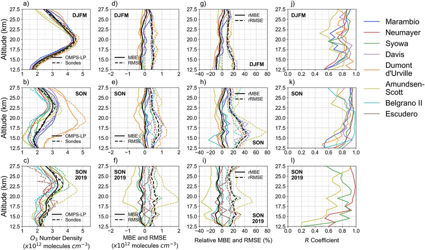
www.nature.com/scientificreports/
stratospheric ozone will be determined not only by the decline in ODSs but also by the increase in greenhouse
gases (GHGs), Antarctic stratospheric ozone is expected to recover back to the 1980 level in the 2 060s10.
Ozone also plays a role in the radiative budget, affecting the atmospheric circulation and climate. Even small
variations in the distribution of trace gases, like ozone, can significantly impact the radiative forcing of the Earth’s
climate and are of key importance for understanding climate c hange14. Recent atmospheric circulation changes
in the southern hemisphere have been attributed to rising greenhouse-gas concentrations and Antarctic ozone
depletion15–19. The acceleration and deceleration of the Brewer-Dobson circulation (BDC) have also been linked
with changes in the ozone abundance over Antarctica20,21. Therefore, a better understanding of the transport
related processes that control the concentrations of radiatively and chemically active species like ozone is of
great interest.
Predicting the radiative forcing due to stratospheric ozone recovery and related processes during this century
also requires detecting changes in the vertical distribution of ozone22. In this endeavor, satellite-derived estimates
play a key role, especially when ground based measurements are scarce. Numerous efforts have focused on the
validation of satellite estimates of the total ozone c olumn23–30. Less attention has been paid to ozone profiles, such
as those produced by the Ozone Mapping and Profiler Suite (OMPS), aboard the Suomi National Polar-orbiting
Partnership (Suomi NPP) satellite, orbiting since October 2011. As part of the Joint Polar Satellite System (JPSS)31
of the National Aeronautics and Space Administration (NASA) and the National Oceanic and Atmospheric
Administration (NOAA), the OMPS provides estimates of both total ozone columns and ozone p rofiles31,32.
A method used to evaluate limb profilers is based on the comparison with balloon-borne ozonesondes33. Here,
we present a comparison between “last state” OMPS-LP ozone profiles (version 2.5 algorithm) and balloon-borne
measurements of the vertical distribution of ozone based on the Electrochemical Concentration Cell (ECC)
method. Balloon-borne ozonesondes were launched from 8 Antarctic stations over the period 2012–2020. Our
comparisons focus on the layer from 12.5 to 27 km (within which satellite-derives profiles and balloon-borne
data overlap) and include ozone profiles retrieved during the Sudden Stratospheric Warming (SSW) event reg-
istered in Spring 2 01934–37. Comparisons consider two periods: September–October–November (SON), when
the Antarctic ozone hole occurs, and December-January–February-March (DJFM), when the ozone abundance
returns to nearly normal values. OMPS-LP data are not available over Antarctica from April to August.
Methods
Satellite‑derived estimates. The OMPS is a suite of three detectors measuring solar radiances scattered
by the atmosphere and solar irradiance in overlapping spectral ranges. These sensors are the OMPS Nadir Map-
per (OMPS-NM) for total ozone column measurements, the OMPS Nadir Profiler (OMPS-NP) for low vertical
resolution ozone profiles (12 Umkehr Layers), and the OMPS Limb Profiler (OMPS-LP) for high vertical resolu-
tion ozone profiles with a vertical range of 12.5–60 km.
The OMPS-LP instrument is a limb sensor type, which observes the “edge” of the Earth´s atmosphere (or
earth’s limb). The closest approach of the sensor line of sight to the Earth´s surface is referred to as the tangent
point; this is the point where the sensor line of sight intersects an Earth radius vector at a right angle and where
the retrieval algorithms calculate the ozone amounts38. The limb view tangent points pass each geographic loca-
tion approximately 7 min after they are viewed by the nadir instrument. The OMPS-LP produces 160–180 limb
measurements per orbit, with 14–15 orbits per day39,40, and 19 s as the record frequency (125 km along-track
motion). The limb measurements consist of the detection of scattered radiances in the line of sight, which then
lead to ozone abundances through the use of an iterative procedure that involves a radiative transfer model41–44.
The OMPS-LP Charge Coupled Device (CCD) detector provides measurements every 1.1 km with 2.1 km verti-
cal resolution. The expected precision for ozone retrievals is better than 20% (or 0.1 ppmv) for elevations lower
than 25 km and 5–10% for elevations from 25–50 k m38.
Three algorithm versions for ozone LP retrievals have been proposed since 2012, with the first version released
just after the beginning of operations, a second version in 2014, and version 2.5, released in 2 01739. Data from
the latter version were obtained from the NASA Goddard Space Flight Center web site (Aura Validation Data
Center)32,45.
Balloon‑borne data. Ozone profiles can also be measured from Electrochemical Concentration Cell
(ECC) ozonesondes. Balloon-borne ozonesondes have been regularly launched from eight Antarctic stations
(see Fig. 1 and Table 1), over the period 2012–2019. These data are available from the World Ozone and UV
Data Center (WOUDC) and the Network for the Detection of Atmospheric Composition Change (NDACC).
Additional ozone profiles were obtained from a campaign at Escudero Station on King George Island (62.2oS,
58.9oW) conducted in spring 2019 in the frame of the SouthTRAC-Halo project and during a SSW event reg-
istered in Spring 2 01934–37. During that special campaign period, 16 ECC ozonesondes, connected to GRAW
DFM-09 radiosondes were launched.
Balloon-borne ozonesondes (attached to a radiosonde) allow for measurements of the vertical distribution of
ozone concentration, temperature, relative humidity (RH), pressure, and winds up to about 30 km. This system is
considered to be the most accurate manner to measure high vertical resolution profiles46. The ECC ozonesondes
systems are mainly composed of a battery-powered gas-sampling pump and an ozone sensor made of two elec-
trodes immersed in potassium iodide (KI) solutions of different concentrations, contained in separate cathode
and anode chambers. The measurement is based on the titration of ozone in the KI sensing solution, producing
an electrical signal from the difference in concentration of the KI-solution between the c hambers47,48. The detec-
tion limit of ECC ozonesondes is typically less than 2 ppbv, while the associated uncertainty is about 10% in the
troposphere and 5% in the stratosphere up to 10 hPa, and 5–25% between 10 and 3 h Pa49–55.
Scientific Reports | (2021) 11:4288 | https://doi.org/10.1038/s41598-021-81954-6 2
Vol:.(1234567890)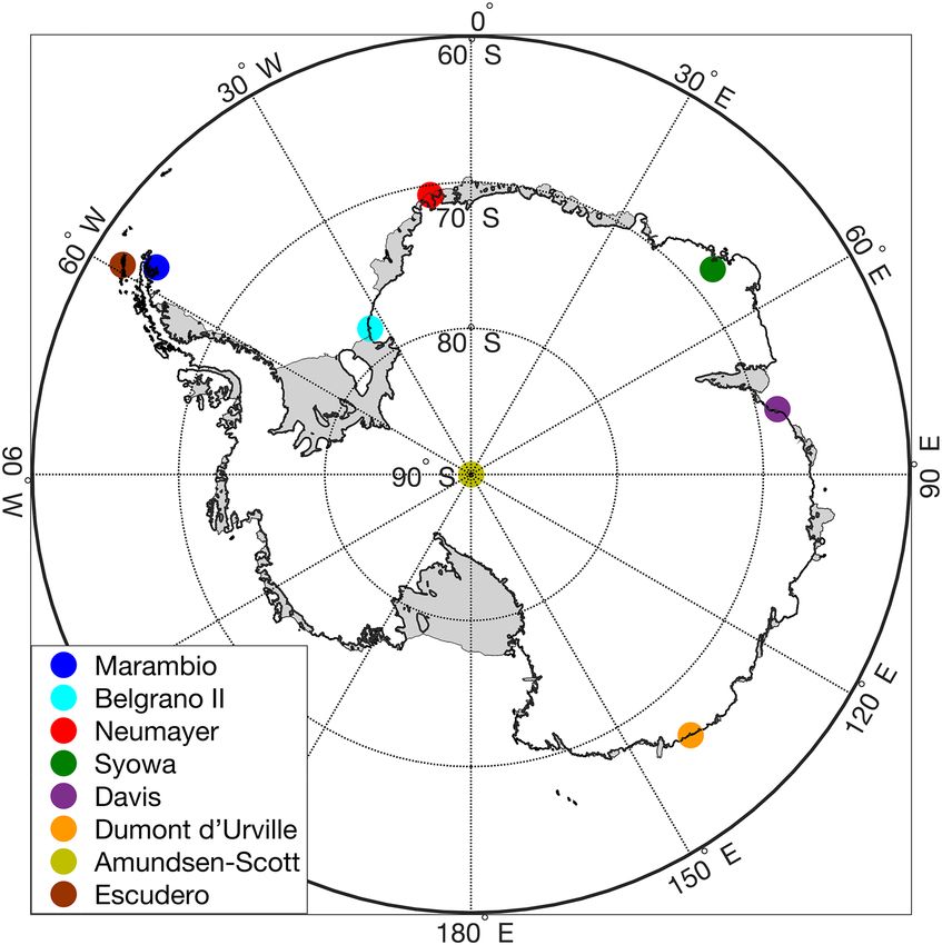
www.nature.com/scientificreports/
Figure 1. Balloon-borne ozonesonde launch sites. Map was generated by using Python’s Matplotlib Library
(version 3.3.3; https://matplotlib.org/users/installing.html)63.
Comparison criteria. Following prior e fforts32,40, we adopted spatial and temporal requirements for the
OMPS-LP and ozonesonde comparison studies. Satellite profiles should be less than 500 km from the ozone-
sonde launch site, and within a time span of ± 12 h. For Amundsen-Scott Station’s sondes, the required distance
was increased to 1000 km due to the orbit track of the OMPS-LP (the average distance is 960 km in the case
of the South Pole40). Comparisons focus on the layer from 12.5 to 27.5 km (within which satellite-derived and
balloon-borne data overlap). Since OMPS-LP data from mid-April to late August are not available over Antarc-
tica, comparisons were conducted over two periods: September–October–November (SON) when the Antarctic
ozone hole occurs, and December-January–February–March (DJFM) when the ozone abundance returns to
nearly normal values. In addition, we also compared ozone profiles retrieved during the SSW event registered
over the period SON 2 01934–37. Before the comparisons, ozonesonde profiles were interpolated to a common
5-m vertical grid and then convolved with a Gaussian averaging kernel over a 1 km range around each sonde
grid point.
For each station and at each altitude, we computed the mean bias error (MBE) and the root mean square
error (RMSE) of OMPS-LP-derived estimates of ozone relative to balloon-borne data; the correlation coefficient
(R) at each altitude was also calculated. Moreover, we computed at each altitude the correlation between some
Scientific Reports | (2021) 11:4288 | https://doi.org/10.1038/s41598-021-81954-6 3
Vol.:(0123456789)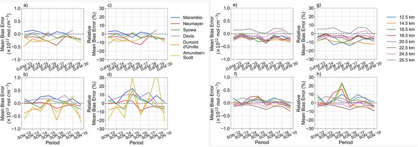
www.nature.com/scientificreports/
DJFM
Station Latitude Longitude Data Network Period Profiles 2013–2020 SON 2012–2018 SON 2019
Marambio − 64.24 − 56.63 WOUDC 2012–2020 128 47 81 0
Belgrano II − 77.87 − 34.63 NDACC 2016–2020 19 0 15 4
Neumayer − 70.67 − 8.27 NDACC 2012–2020 312 114 179 19
Syowa − 68.30 49.64 WOUDC 2012–2020 148 52 83 13
Davis − 68.57 77.97 WOUDC 2012–2020 94 34 60 0
Dumont
− 66.66 139.91 NDACC 2012–2020 53 16 37 0
d’Urville
Amundsen-Scott − 89.98 139.28 NDACC 2012–2020 129 74 49 6
Escudero − 62.20 − 58.92 – 2019 5 0 0 5
Table 1. Number of ozone profiles considered in the comparisons, over the periods: DJFM 2013–2020, SON
2012–2018, and SON 2019.
OMPS-LP parameters and the relative differences (between the OMPS-LP-derived and balloon-borne data of
ozone); the following OMPS-LP parameters were considered: time difference between satellite readings and
ozonesonde launch, distance to the station, solar zenith angle (SZA), single scattering angle (SSA), tropopause
altitude, surface reflectance, and cloud height. Finally, we built up scatter plots formed by clustering, regardless
of altitude, OMPS-LP-derived and balloon-borne data of ozone. The results for each station are shown in the
Supplementary Material.
Balloon-borne data are reported in partial pressure units (mPa), while OMPS-LP ozone profiles retrievals
are presented in number density units (number of ozone molecules per cubic centimeter). The transformation
from partial pressure units into number density units is straightforward if temperature profiles are available.
Therefore, we began our analyses by checking the consistency of balloon-borne measurements of temperature
using Modern-Era Retrospective analysis for Research and Applications, Version 2 (MERRA-2)56. MERRA-2
data are embedded in the OMPS-LP dataset. Reliable temperature profiles are needed for the transformation
from partial pressure units into number density units of the sonde readings. At each altitude, we computed MBE,
RMSE and R between balloon-borne measurements of temperature and MERRA-2 d ata56. As shown in Fig. S1,
the differences between balloon-borne measurements of the temperature and reanalysis data are generally lower
than 0.5%. The MBE was greater (but still less than 1%) in the case of Amundsen-Scott Station’s sondes, which
can be attributed to the distance between the orbit track and the launch site.
Results
Figure 2a,b show the significant seasonal changes that the vertical distribution of ozone exhibits over Antarctica.
Within the layer from 12.5 to 22 km the concentration of ozone is on average about 30–50% lower during SON
than during DJFM (except in the case of the Dumont d’Urville station that is often outside the polar vortex).
Differences between balloon-borne and OMPS-LP-derived data change with the season, especially at altitudes
lower than 22 km.
Most of the profiles exhibit a good agreement at altitudes higher than 22 km (see Fig. 2d–e,g–h). The relative
mean bias errors (rMBE) are generally lower than ± 10% within the layer from 22 to 27.5 km except in the case
of the Amundsen-Scott Station, which can be attributed to the long distance between the station and the orbit
track. Within the layer from 12.5 to 22 km, the biases of the OMPS-LP-derived estimates are season-dependent.
As shown in Fig. 2g, OMPS-LP-derived estimates generally exhibit a negative mean bias error (up to about
-20%) during DJFM (i.e. when the ozone concentration reach higher values). However, as shown in Fig. 2h, mean
bias errors of OMPS-LP-derived estimates within the same layer (12.5–22 km) are not predominately negative
during SON (i.e. when the Antarctic ozone depletion peaks); negative biases (up to about -10%) are apparent
especially in the case of the Dumont d’Urville station (which is often outside the polar vortex) while positive
biases (up to about + 15%) were found in the case of Marambio, and Davis stations (see Fig. 2h).
RMSE values tend to be larger (about 20%) in the lower stratosphere (12.5–17.5 km) and smaller (about 10%)
within higher layers during DJFM (see Fig. 2g). RMSE values are significantly larger (even greater than 40%)
during SON, especially within the layer from 12.5 to 22 km (see Fig. 2h). These relatively high RMSE values
were expected for stations within the polar vortex (such as Amundsen-Scott) since during the ozone hole season
(SON), the ozone concentration within this layer (12.5–22 km) can even fall below the detection limit of the
ozonesondes9, which is about 10 ppbv57.
As shown in Figs. 2j,k, the correlation between the balloon-borne and OMPS-LP-derived ozone concentra-
tions is generally high, especially during the SON period and at altitudes higher than 17.5 km, for which R
values greater than 0.9 are generally found. An exception is again observed in the case of the Amundsen-Scott
Station, which can be attributed to the long distance between the station and the orbit track. At lower altitudes
(within the layer from 12.5 to 17.5 km), R values are somehow lower (but still higher than 0.55), regardless of
the season. Lower correlations are nevertheless expected at lower altitudes, as satellite products tend to be more
reliable at higher altitudes.
The differences between balloon-borne and OMPS-LP-derived profiles during the SSW event during SON
2019 are similar to those observed during other SON periods. As shown in Fig. 2 (third row), the profiles of
MBE, RMSE and R computed during SON 2019 tend to follow those computed over the period SON 2012–2018.
Scientific Reports | (2021) 11:4288 | https://doi.org/10.1038/s41598-021-81954-6 4
Vol:.(1234567890)www.nature.com/scientificreports/
Figure 2. Comparison between OMPS-LP-derived and balloon-borne data of ozone over the period DJFM
2013–2020 (first row), over the period SON 2012–2018 (second row), and over the period SON 2019 (third
row). (a–c) Mean profiles per station. The solid line stands for the mean computed from OMPS-LP-derived
estimates of ozone and the dashed line stands for the mean computed from balloon-borne measurements of
ozone. The mean was computed from the cluster formed with profiles from Marambio, Neumayer, Syowa, Davis
and Dumont d’Urville stations. Amundsen-Scott Station data were not considered for computing the mean due
to the long distance between the station and the orbit track; Belgrano II and Escudero data were not considered
either due to the low temporal distribution of the balloon-borne ozonesondes. (d–f) Mean Bias Error (MBE,
solid line) and Root Mean Square Error (RMSE, dashed line) relative to balloon-borne data. (g–i) Relative Mean
Bias Error (rMBE, solid line) and Relative Root Mean Square Error (rRMSE, dashed line). (j–l) Correlation
coefficient (R) profile; data corresponding to Belgrano II and Escudero were not considered since few balloon-
borne ozonesondes during SON 2019 fulfilled the adopted comparison criteria. 263, 440 and 37 ozone profiles
were compared over the periods DJFM 2013–2020, SON 2012–2018 and SON 2019, respectively. Plots were
generated by using Python’s Matplotlib Library63.
However, there are interesting differences. When comparing Fig. 2h,i, it can be observed that the RMSE values
are, within the layer from 12.5 to 22 km (i.e. the most depleted during the ozone hole season), generally lower
during SON 2019 than during SON 2012–2018. In fact, within this layer, RMSE values were closer to those
observed over the period DJFM 2013–2020 (Fig. 2g) than to those observed over the period SON 2012–2018
(Fig. 2h). This is likely due to the fact that the SSW event during SON 2019 led to the smallest ozone hole
observed in decades (i.e. ozone concentrations were closer to those registered during DJFM). Moreover, when
comparing Figs. 2k,l, it can be observed that the R values were found to be lower during SON 2019 than during
SON 2012–2018 within the layer from 12.5 to 15.5 km, which can be attributed to the relatively low number of
ozonesondes that fulfilled the comparison criteria.
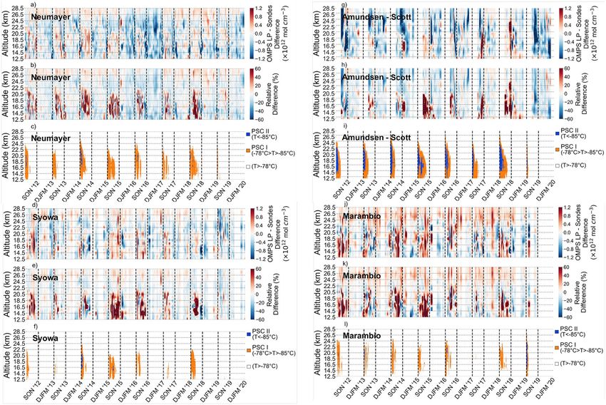
A detailed representation of the relative difference between balloon-borne and OMPS-LP-derived data
is shown in Fig. 3 for four stations, Neumayer (Fig. 3a–c), Syowa (Fig. 3d–f), Amundsen-Scott (South Pole,
Fig. 3g–i) and Marambio (Fig. 3j–l). Periods and altitudes at which the temperature favors the formation of polar
stratospheric clouds (PSC), type I and type II, are also shown. As expected, larger relative differences are observed
during the ozone hole season (SON) when the lowest ozone concentrations occur. Once the ozone hole begins,
the total ozone column drops rapidly at a rate of 3–5 DU per day, with nearly all of the ozone disappearing by
late September within the layer from 14 to 22 k m58, which generally led to large relative biases. Larger relative
differences are also observed after the disappearance of the PSCs. This is attributable to the polar vortex that
keeps the ozone-depleted air isolated from the surrounding ozone-rich air. The sharp meridional ozone gradient
(from outside to inside of the polar vortex) may also negatively affect the agreement between balloon-borne and
OMPS-LP-derived data, especially in the case of observations conducted close to the edge of the polar vortex. As
expected, relative differences within the layer from 12.5 to 22 km peaked at 55% during the ozone hole season in
2015 (the greatest ozone hole of the last decade59). The prevalence of the red color in the heatmap within the layer
from 12.5 to 22 km during the ozone hole season suggests that OMPS-LP-derived estimates tend to overestimate
the ozone concentration in case of extremely low ozone abundances.
Scientific Reports | (2021) 11:4288 | https://doi.org/10.1038/s41598-021-81954-6 5
Vol.:(0123456789)www.nature.com/scientificreports/
Figure 3. Heatmap of the differences (absolute and relative) between OMPS-LP-derived estimates and balloon-
borne measurements; blank spaces indicates periods within which no sondes fulfilling the comparison criteria
were available. Periods and altitudes at which the temperature favors the formation of polar stratospheric
clouds (PSC) are shown below the heatmaps; temperature profiles from sondes were used. Dashed vertical lines
separate different periods per year (DJFM and SON). (a–c) Neumayer; (d–f) Syowa; (g–i) Amundsen-Scott; and
(j–l) Marambio. Plots were generated by using Python’s Matplotlib L ibrary63.
Figure 4. Time series of the absolute and relative mean bias errors (MBE) of OMPS-LP-derived estimates of
the ozone (relative to balloon-borne data) computed over the DJFM period (first row) and over the SON period
(second row). (a–d) per station; (e–h) per altitude. Plots were generated by using Python’s Matplotlib Library63.
Scientific Reports | (2021) 11:4288 | https://doi.org/10.1038/s41598-021-81954-6 6
Vol:.(1234567890)www.nature.com/scientificreports/
max min max min
MBE max MBE MBE— min MBE MBE— RMSE max RMSE RMSE— min RMSE RMSE—
(× 1012 mol cm- (× 1012 mol cm- Altitude (× 1012 mol cm- Altitude RMSE (× 1012 mol cm- (× 1012 mol cm- Altitude (× 1012 mol cm- Altitude
Station MBE (%) 3
) 3
) (km) 3
) (km) (%) 3
) 3
) (km) 3
) (km) R
DJFM
Marambio 1.1 0.04 0.39 25.5 − 0.22 12.5 14 0.44 0.58 17.5 0.25 27.5 0.92
Belgrano
– – – – – – – – – – – – –
II
Neumayer − 5.8 − 0.20 0.06 27.5 − 0.35 15.5 13 0.42 0.56 15.5 0.22 27.5 0.93
Syowa − 3.0 − 0.10 0.14 26.5 − 0.23 22.5 11 0.37 0.51 19.5 0.25 27.5 0.94
Davis − 1.1 − 0.04 0.26 26.5 − 0.28 14.5 13 0.42 0.61 14.5 0.29 27.5 0.92
Dumont
− 6.2 − 0.22 0.10 25.5 − 0.45 16.5 15 0.53 0.77 17.5 0.27 27.5 0.91
d’Urville
Amund-
− 6.7 − 0.22 0.03 12.5 − 0.38 21.5 16 0.54 0.73 17.5 0.28 27.5 0.90
sen-Scott
Escudero – – – – – – – – – – – – –
SON
Marambio 5.7 0.15 0.30 25.5 − 0.01 21.5 27 0.70 1.05 18.5 0.31 27.5 0.86
Belgrano
0.3 0.01 0.19 20.5 − 0.43 14.5 24 0.47 0.64 14.5 0.29 16.5 0.94
II
Neumayer − 2.7 − 0.06 0.11 27.5 − 0.22 23.5 21 0.44 0.65 15.5 0.23 26.5 0.93
Syowa 0.4 0.01 0.14 20.5 − 0.19 22.5 21 0.47 0.72 16.5 0.18 27.5 0.92
Davis 5.6 0.14 0.40 26.5 − 0.02 17.5 26 0.68 1.12 18.5 0.37 14.5 0.88
Dumont
− 6.1 − 0.24 0.06 12.5 − 0.66 20.5 23 0.91 1.29 16.5 0.47 27.5 0.86
d’Urville
Amund-
− 7.5 − 0.17 0.15 12.5 − 0.43 24.5 34 0.79 1.01 23.5 0.36 12.5 0.85
sen-Scott
Escudero – – – – – – – – – – – – –
SON 2019
Marambio – – – – – – – – – – – – –
Belgrano
− 6.6 − 0.16 0.06 20.5 − 0.42 15.5 11 0.28 0.45 15.5 0.09 27.5 0.97
II
Neumayer − 4.5 − 0.11 0.06 21.5 − 0.48 15.5 14 0.35 0.65 15.5 0.25 25.5 0.94
Syowa − 7.0 − 0.22 0.01 20.5 − 0.46 22.5 18 0.58 1.01 19.5 0.28 12.5 0.88
Davis – – – – – – – – – – – – –
Dumont
– – – – – – – – – – – – –
d’Urville
Amund-
− 22 − 0.72 0.21 12.5 − 1.30 18.5 34 1.10 1.99 19.5 0.25 13.5 0.78
sen-Scott
Escudero 1.6 0.04 0.54 27.5 − 0.42 18.5 20 0.51 0.86 15.5 0.29 24.5 0.89
Table 2. Mean Bias Error (MBE) and Root Mean Square Error (RMSE) over the periods: DJFM 2013–2020,
SON 2012–2018 and SON 2019. Maximum and minimum values of the MBE and RMSE profiles are also
shown. Since few profiles were available, data are not shown for some stations.
Figure 4 presents the time series of the mean bias errors of OMPS-LP-derived estimates of ozone relative to
balloon-borne data. OMPS-LP-derived estimates generally exhibit a negative mean bias error within the layer
12.5–22 km during DJFM (see Fig. 2g). The same negative mean bias error is apparent in Fig. 4g, which also
suggests a small negative drift at lower altitudes (see for example the 14.5 km level). Prior efforts32 have tested
OMPS-LP data (over 5.5 years) with profiles retrieved from the Odin Optical Spectrograph and InfraRed Imaging
System (OSIRIS)60 and from the Aura Microwave Limb Sounder (MLS)61. Although Kramarova et al.32 found
no significant drift when comparing OMPS-LP data with profiles retrieved from MLS, they did find a negative
drift below 20 km when comparing OMPS-LP data with profiles retrieved from OSIRIS over Antarctic latitudes
(90°–60° S). These results underline the challenges for the detection of drifts, especially over Antarctic latitudes
(90°–60° S), where ozone is subjected to a significant year-to-year variability. In our case, the evaluation period
(2012–2020) is likely too short for confirming/discarding a drift using balloon-borne measurements as reference.
During SON (when the ozone hole occurs), the relative mean bias errors were occasionally large (up to + 30%)
within the layer from 12.5 to 22 km (see Fig. 4). This is likely related to the relatively low concentration of ozone
within this layer over stations inside the polar vortex. Nevertheless, Fig. 4b shows that the absolute mean bias
errors of OMPS-LP-derived estimates of the ozone (relative to balloon-borne data) are generally lower than
0.2 × 10¹² molecules/cm3 (about 0.3 ppmv). Although according to Fig. 4b, the mean bias errors of OMPS-LP-
derived estimates of ozone (relative to balloon-borne data) show some stability at the 0.3 ppmv level, it is worth
highlighting that such a level may only allow for the detection of changes at time scales longer than decades.
In the Supplementary Material we present, for each launch site, the profiles of MBE, RMSE and R computed by
comparing balloon-borne and OMPS-LP-derived data. In Table 2 we show the maximum and minimum values
of the MBE and RMSE obtained from the corresponding profiles for each launch site. Also, for each altitude, we
present in the Supplementary Material the correlations between the relative differences (between balloon-borne
and OMPS-LP-derived data of ozone) and the following parameters: time difference between satellite readings
Scientific Reports | (2021) 11:4288 | https://doi.org/10.1038/s41598-021-81954-6 7
Vol.:(0123456789)www.nature.com/scientificreports/
and ozonesonde launch, distance to the station, SZA, SSA, tropopause altitude, surface reflectance, and the
cloud height. These correlations may suggest potential issues that affect the retrieval algorithm. The following
correlations were identified:
• significant correlations between the relative ozone differences and the surface reflectance were found during
DJFM. The correlation is often positive for Amundsen-Scott (where R peaked at 0.62 at 27.5 km) but con-
stantly negative for Syowa (where R peaked at − 0.55 at 20.5 km) and for Marambio (especially at altitudes
higher than 17 km; in the case of Marambio, R peaked at − 0.40 at 24.5 km). Although correlations were
found to be generally smaller during SON. Our results suggest that further efforts should be undertaken in
future algorithm updates in order to minimize the sensitivity of the retrieved ozone profile to the underlying
scene reflectance32;
• positive correlations between the relative ozone differences and the cloud height exists for Syowa during
both SON and DJFM (in the case of Syowa, R peaked at 0.38 at 23.5 km during SON and at 0.34 at 21.5 km
during DJFM); positive correlation were also found for Belgrano (where R peaked at 0.56 at 18.5 km during
SON). During DJFM, negative correlations were found for Dumont d’Urville (where R peaked at − 0.53 at
23.5 km) as well as for Davis (where R peaked at − 0.34 at 22.5 km). Significant correlations are limited to
only specific altitudes at other stations. The OMPS-LP algorithm retrieves ozone profiles from cloud top to
37.5 km; if no cloud is identified, the retrieval lower limit is set to 12.5 km. However, cloud detection over
the bright Antarctic surfaces is particularly challenging in the ultraviolet and visible spectral range used by
the OMPS-LP algorithm. The identified correlations between the relative ozone differences and the cloud
height suggest that, in the case of Antarctica, there is still room for improvements in the cloud detection
algorithm62;
• slightly positive correlations between the relative ozone differences and the SZA were found during SON for
Dumont d’Urville, Amundsen-Scott and Belgrano. In contrast, correlations are consistently negative dur-
ing DJFM for the majority of the stations e.g., for Neumayer and Syowa (especially at altitudes higher than
15.5 km), as well as for Marambio (where R peaked at − 0.53 at 23.5 km) and Davis (where R peaked at − 0.56
at 24.5 km). The correlation was also negative during SON for Syowa (where R peaked at − 0.44 at 25.5 km).
The dependence on the SZA is typical for satellite products of the total ozone column and often emerges
from validation efforts based on ground-based observations (as ground observations are more uncertain
for low solar elevations)25. However, the influence of the SZA on ozone differences was unexpected in our
case because ozonesonde data do not depend on the SZA. Therefore, straightforward conclusions cannot be
drawn on this issue;
• positive correlations between the relative ozone differences and the tropopause altitude were found, mainly
at altitudes lower than 20 km. This correlation was particularly clear during SON in the case of Amundsen-
Scott and Belgrano II where R peaked for both stations at 15.5 km at 0.61 and 0.78, respectively. Nevertheless,
conclusions on this issue remain challenging since results for Belgrano II are based on few ozone data pairs
(15 over the period 2012–2018) while for Amundsen-Scott the distance between satellite observations and
ozonesondes is on average about two times larger than for other stations;
• negative correlations between relative ozone differences and the SSA were detected especially during DJFM
at the upper altitudes; e.g., during DJFM for Neumayer (where R peaked at − 0.34 at 23.5 km), Marambio
(where R peaked at − 0.50 at 23.5 km), Syowa (where R peaked at − 0.30 at 23.5 km), and Davis (where R
peaked at − 0.55 at 24.5 km).
Distance and time differences were found to marginally affect the relative ozone differences (except for
Dumont d’Urville and Belgrano for specific altitude ranges and seasons).
Summary and conclusions
Ozone plays an important role in the radiative budget, affecting the atmospheric circulation and climate. Even
small variations in the distributions of trace gases, like ozone, can significantly impact the radiative forcing of
Earth’s climate and are of key importance for understanding climate change. Therefore, a better understanding
of the transport related processes that control the concentrations of radiatively and chemically active species
like ozone is of great interest.
Predicting the radiative forcing due to stratospheric ozone recovery and related processes during this century
requires detecting changes in the vertical distribution of ozone. However, trend detection in the case of ozone is
complicated by the climate variability (in the season 2019–2020 one of the smallest ozone holes occurred over
Antarctica and one of the largest ozone loss events occurred over the Arctic). Overcoming these challenges
requires improving the accuracy of satellite-derived estimates. In this endeavor, the validation of satellite prod-
ucts plays a key role.
Here, we have carried out a systematic comparison between “last state” OMPS-LP ozone profiles (version
2.5 algorithm) and balloon-borne measurements of the ozone abundance gathered by ECC-type ozonesondes.
The OMPS-LP instrument, aboard the Suomi NPP satellite, provides estimates of both the total ozone column
and ozone profiles since October 2011. The balloons were launched from 8 Antarctic stations over the period
2012–2020. Comparisons focused on the layer from 12.5 to 27.5 km and were conducted over two periods: SON
and DJFM.
We found that most of the profiles exhibit a good agreement within the layer from 22 to 27.5 km, within which
MBE values are generally lower than ± 10% (except in the case of the Amundsen-Scott Station). Within the layer
from 12.5 to 22 km, the biases of the OMPS-LP-derived estimates are season-dependent; MBE values remain
Scientific Reports | (2021) 11:4288 | https://doi.org/10.1038/s41598-021-81954-6 8
Vol:.(1234567890)www.nature.com/scientificreports/
in the same range (± 10%) as at higher altitudes during the ozone hole season (SON), but MBE values become
predominantly negative (up to about − 20%) during DJFM (i.e. when the ozone concentration reaches higher
values). Nevertheless, we found that relative to balloon-borne data, MBE values of OMPS-derived Antarctic
ozone profiles are generally less than 0.3 ppmv.
We also found that, during DJFM, RMSE values tend to be larger (about 20%) in the lower stratosphere
(12.5–17.5 km) and smaller (about 10%) within higher layers (17.5–27.5 km). However, during the ozone hole
season (SON), RMSE values exhibit larger figures (even greater than 40%) within the layer from 12.5 to 22 km,
especially in the case of stations within the polar vortex (such as Amundsen-Scott).
Our results suggest that the differences between balloon-borne and OMPS-derived Antarctic ozone profiles
are generally within the bounds defined by the uncertainties of both satellite-derived and balloon-borne data.
The associated uncertainty of ECC ozonesonde measurements is about 10% in the troposphere and 5% in the
stratosphere up to 10 hPa, and 5–25% between 10 and 3 h Pa49–55, while the expected precision for ozone retrievals
is better than 20% for elevations lower than 25 km and 5–10% for elevations from 25–50 k m38.
The total ozone over Antarctic latitudes (90°-60°S) in the months of September and October is increasing at
a rate of about 6–8% per decade (see Fig. 4.15 in Scientific Assessment of Ozone Depletion10). If the Antarctic
stratospheric ozone returns to 1980 values in the 2060s as projected by W MO10, ozone concentrations at 20 km
should increase in the next decades at a rate in the range from 0.2 to 0.3 ppmv/decade. This means that, as the
ozone hole closes, the inter-decadal increases in the ozone concentration expected in the upcoming decades at
altitudes of about 20 km over Antarctica are similar to the mean bias error of OMPS-derived ozone concentra-
tions (generally less than 0.3 ppmv relative to balloon-borne measurements).
Relative to balloon-borne measurements, satellite-derived data exhibit no major drift, but the evaluation
period (2012–2020) is likely too short for confirming/discarding a drift. Significant correlations were found
between the satellite estimates biases and the tropopause altitude, the cloud height, and the surface reflectance.
These correlations suggest that further efforts to minimize the retrieval errors should focus on improving the
sensitivity of the algorithm to the underlying Antarctic conditions.
Data availability
Satellite-derived ozone profiles were obtained from the NASA Goddard Space Flight Center web site (Aura
Validation data center): https: //gs614- avdc1- pz.gsfc.nasa.gov/pub/data/satell ite/Suomi_ NPP/L2OVP/ LP-L2-O3-
DAILY/ . Balloon-borne ozonesonde data were obtained from the World Ozone and UV Data Center (WOUDC:
https://woudc.org/data/explore.php?lang=en) and the Network for the Detection of Atmospheric Composition
Change (NDACC: https://www.ndaccdemo.org). Additional datasets and codes are available from the corre-
sponding author on reasonable request.
Received: 30 August 2020; Accepted: 11 January 2021
References
1. Lakkala, K. et al. New continuous total ozone, UV, VIS and PAR measurements at Marambio, 64° S, Antarctica. Earth Syst. Sci.
Data 12, 947–960 (2020).
2. McKenzie, R. et al. Success of Montreal protocol demonstrated by comparing high-quality UV measurements with “world avoided”
calculations from two chemistry-climate models. Sci. Rep. 9, 12332 (2019).
3. Barnes, P. W. et al. Ozone depletion, ultraviolet radiation, climate change and prospects for a sustainable future. Nat. Sustain. 2,
569–579 (2019).
4. Cordero, R. R. et al. UV irradiance and albedo at Union Glacier Camp (Antarctica): a case study. PLoS ONE 9, e90705 (2014).
5. Cordero, R. R. et al. Satellite-derived UV climatology at Escudero station Antarctic Peninsula. Antarct. Sci. 25, 791–803 (2013).
6. Seckmeyer, G. & McKenzie, R. L. Increased ultraviolet radiation in New Zealand (45 S) relative to Germany (48 N). Nature
359(6391), 135–137 (1992).
7. Farman, J. C., Gardiner, B. G. & Shanklin, J. D. Large losses of total ozone in Antarctica reveal seasonal ClOx/NOx interaction.
Nature 315, 207–210 (1985).
8. Solomon, S., Garcia, R. R., Rowland, F. S. & Wuebbles, D. J. On the depletion of Antarctic ozone. Nature 321(6072), 755–758 (1986).
9. Grooß, J.-U., Brautzsch, K., Pommrich, R., Solomon, S. & Müller, R. Stratospheric ozone chemistry in the Antarctic: what deter-
mines the lowest ozone values reached and their recovery?. Atmos. Chem. Phys. 11, 12217–12226 (2011).
10. WMO (World Meteorological Organization). Scientific Assessment of Ozone Depletion: 2018, Global Ozone Research and Moni-
toring Project-Report No. 58 (2018).
11. Strahan, S. E. & Douglass, A. R. Decline in Antarctic ozone depletion and lower stratospheric chlorine determined from aura
microwave limb sounder observations. Geophys. Res. Lett. 45, 382–390 (2018).
12. Weber, M. et al. Total ozone trends from 1979 to 2016 derived from five merged observational datasets—the emergence into ozone
recovery. Atmos. Chem. Phys. 18, 2097–2117 (2018).
13. Solomon, S. et al. Emergence of healing in the Antarctic ozone layer. Science 353, 269–274 (2016).
14. Riese, M. et al. Impact of uncertainties in atmospheric mixing on simulated UTLS composition and related radiative effects. J.
Geophys. Res. Atmos. 117, D16305 (2012).
15. Damiani, A. et al. Connection between Antarctic Ozone and climate: interannual precipitation changes in the southern hemisphere.
Atmosphere 11, 579 (2020).
16. Lenaerts, J. T. M., Fyke, J. & Medley, B. The signature of ozone depletion in recent Antarctic precipitation change: a study with the
community earth system model. Geophys. Res. Lett. 45, 12931–12939 (2018).
17. Polvani, L. M., Waugh, D. W., Correa, G. J. P. & Son, S. W. Stratospheric ozone depletion: The main driver of twentieth-century
atmospheric circulation changes in the Southern Hemisphere. J. Clim. 24, 795–812 (2011).
18. Previdi, M. & Polvani, L. M. Climate system response to stratospheric ozone depletion and recovery. Q. J. R. Meteorol. Soc. 140,
2401–2419 (2014).
19. Thompson, D. W. J. et al. Signatures of the Antarctic ozone hole in Southern Hemisphere surface climate change. Nat. Geosci. 4,
741–749 (2011).
20. Fu, Q., Solomon, S., Pahlavan, H. A. & Lin, P. Observed changes in Brewer-Dobson circulation for 1980–2018. Environ. Res. Lett.
14, 114026 (2019).
Scientific Reports | (2021) 11:4288 | https://doi.org/10.1038/s41598-021-81954-6 9
Vol.:(0123456789)www.nature.com/scientificreports/
21. Aschmann, J. et al. On the hiatus in the acceleration of tropical upwelling since the beginning of the 21st century. Atmos. Chem.
Phys. 14, 12803–12814 (2014).
22. Harris, N. R. P. et al. Past changes in the vertical distribution of ozone—part 3: analysis and interpretation of trends. Atmos. Chem.
Phys. 15, 9965–9982 (2015).
23. Paschou, P., Koukouli, M.-E., Balis, D., Lerot, C. & Van Roozendael, M. The effect of considering polar vortex dynamics in the
validation of satellite total ozone observations. Atmos. Res. 238, 104870 (2020).
24. Antón, M. et al. Total ozone column derived from GOME and SCIAMACHY using KNMI retrieval algorithms: validation against
Brewer measurements at the Iberian Peninsula. J. Geophys. Res. Atmos. 116, D22303 (2011).
25. Damiani, A., De Simone, S., Rafanelli, C., Cordero, R. R. & Laurenza, M. Three years of ground-based total ozone measurements
in the Arctic: Comparison with OMI, GOME and SCIAMACHY satellite data. Remote Sens. Environ. 127, 162–180 (2012).
26. Koukouli, M. E. et al. Geophysical validation and long-term consistency between GOME-2/MetOp-A total ozone column and
measurements from the sensors GOME/ERS-2, SCIAMACHY/ENVISAT and OMI/Aura. Atmos. Meas. Tech. 5, 2169–2181 (2012).
27. Buchard, V. et al. Comparison of OMI ozone and UV irradiance data with ground-based measurements at two French sites. Atmos.
Chem. Phys. 8, 4517–4528 (2008).
28. Eskes, H. J. et al. Retrieval and validation of ozone columns derived from measurements of SCIAMACHY on Envisat. Atmos.
Chem. Phys. Discuss. 5, 4429–4475 (2005).
29. Fioletov, V. E. et al. Performance of the ground-based total ozone network assessed using satellite data. J. Geophys. Res. 113, D14313
(2008).
30. Ialongo, I., Casale, G. R. & Siani, A. M. Comparison of total ozone and erythemal UV data from OMI with ground-based measure-
ments at Rome station. Atmos. Chem. Phys. 8, 3283–3289 (2008).
31. Flynn, L. et al. Performance of the Ozone Mapping and Profiler Suite (OMPS) products. J. Geophys. Res. Atmos. 119, 6181–6195
(2014).
32. Kramarova, N. A. et al. Validation of ozone profile retrievals derived from the OMPS LP version 2.5 algorithm against correlative
satellite measurements. Atmos. Meas. Tech. 11, 2837–2861 (2018).
33. McLinden, C. A. et al. An evaluation of Odin/OSIRIS limb pointing and stratospheric ozone through comparisons with ozone-
sondes. Can. J. Phys. 85, 1125–1141 (2007).
34. Newman, P. A. & Nash, E. R. The unusual southern hemisphere stratosphere winter of 2002. J. Atmos. Sci. 62, 614–628 (2005).
35. Yamazaki, Y. et al. September 2019 Antarctic sudden stratospheric warming: quasi-6-day wave burst and ionospheric effects.
Geophys. Res. Lett. 47, 1–12 (2020).
36. Rao, J., Garfinkel, C. I., White, I. P. & Schwartz, C. The southern hemisphere minor sudden stratospheric warming in September
2019 and its predictions in S2S models. J. Geophys. Res. Atmos. 125, 1–30 (2020).
37. Damiani, A. et al. Changes in the composition of the northern polar upper stratosphere in February 2009 after a sudden strato-
spheric warming. J. Geophys. Res. Atmos. 119, 11429–11444 (2014).
38. Jaross, G. et al. OMPS Limb Profiler instrument performance assessment. J. Geophys. Res. Atmos. 119, 4399–4412 (2014).
39. Kramarova, N. et al. Overview of version 2.5 ozone profile products from the Suomi NPP OMPS Limb Profiler by. Glob. Space-
Based Inter-Calibration Syst. 11, 8–9 (2017).
40. Arosio, C. et al. Retrieval of ozone profiles from OMPS limb scattering observations. Atmos. Meas. Tech. 11, 2135–2149 (2018).
41. Rault, D. F. & Loughman, R. P. The OMPS Limb Profiler environmental data record algorithm theoretical basis document and
expected performance. IEEE Trans. Geosci. Remote Sens. 51, 2505–2527 (2013).
42. Herman, B. M., Caudill, T. R., Flittner, D. E., Thome, K. J. & Ben-David, A. Comparison of the Gauss-Seidel spherical polarized
radiative transfer code with other radiative transfer codes. Appl. Opt. 34, 4563 (1995).
43. Loughman, R. P. et al. Description and sensitivity analysis of a limb scattering ozone retrieval algorithm. J. Geophys. Res. D Atmos.
110, 1–23 (2005).
44. Loughman, R., Flittner, D., Nyaku, E. & Bhartia, P. K. Gauss-Seidel limb scattering (GSLS) radiative transfer model development
in support of the Ozone Mapping and Profiler Suite (OMPS) limb profiler mission. Atmos. Chem. Phys. 15, 3007–3020 (2015).
45. NASA. Goddard Space Flight Center web page (Aura Validation Data Center). Suomi section. https://gs614-avdc1-pz.gsfc.nasa.
gov/pub/data/satellite/Suomi_NPP/L2OVP/LP-L2-O3-DAILY/ (2020).
46. Jiang, Y. B. et al. Validation of Aura Microwave Limb Sounder Ozone by ozonesonde and lidar measurements. J. Geophys. Res.
Atmos. 112, 1–20 (2007).
47. Komhyr, W. D., Barnes, R. A., Brothers, G. B., Lathrop, J. A. & Opperman, D. P. Electrochemical concentration cell ozonesonde
performance evaluation during STOIC 1989. J. Geophys. Res. 100, 9231–9244 (1995).
48. Smit, H. G. J. & Panel for the assessment of standard operation procedures for ozonesondes (ASOPOS). Quality Assurance and
Quality Control for Ozonesonde Measurements in GAW. GAW report 201. vol. 41 (2004).
49. Bodeker, G. E., Boyd, I. S. & Matthews, W. A. Trends and variability in vertical ozone and temperature profiles measured by
ozonesondes at Lauder, New Zealand: 1986–1996. J. Geophys. Res. Atmos. 103, 28661–28681 (1998).
50. Borchi, F., Pommereau, J.-P., Garnier, A. & Pinharanda, M. Evaluation of SHADOZ sondes, HALOE and SAGE II ozone profiles at
the tropics from SAOZ UV-Vis remote measurements onboard long duration balloons. Atmos. Chem. Phys. 5, 1381–1397 (2005).
51. Kerr, J. B. et al. The 1991 WMO international ozonesonde intercomparison at Vanscoy, Canada. Atmos. Ocean 32, 685–716 (1994).
52. Smit, H. G. J. et al. Assessment of the performance of ECC-ozonesondes under quasi-flight conditions in the environmental
simulation chamber: insights from the Juelich Ozone Sonde Intercomparison Experiment (JOSIE). J. Geophys. Res. Atmos. 112,
1–18 (2007).
53. Thompson, A. M. et al. Intercontinental Chemical Transport Experiment Ozonesonde Network Study (IONS) 2004: 1. Summertime
upper troposphere/lower stratosphere ozone over northeastern North America. J. Geophys. Res. Atmos. 112, D12 (2007).
54. Thompson, A. M. et al. Intercontinental Chemical Transport Experiment Ozonesonde Network Study (IONS) 2004: 2. Tropospheric
ozone budgets and variability over northeastern North America. J. Geophys. Res. 112, D12 (2007).
55. Thompson, A. M. et al. Southern Hemisphere Additional Ozonesondes (SHADOZ) 1998–2004 tropical ozone climatology: 3.
Instrumentation, station-to-station variability, and evaluation with simulated flight profiles. J. Geophys. Res. Atmos. 112, D3 (2007).
56. Randles, C. A. et al. The MERRA-2 Aerosol Reanalysis, 1980 onward. Part I: system description and data assimilation evaluation.
J. Clim. 30, 6823–6850 (2017).
57. Vomel, H. & Diaz, K. Ozone sonde cell current measurements and implications for observations of near-zero ozone concentrations
in the tropical upper troposphere. Atmos. Meas. Tech. 3, 495–505 (2010).
58. Hofmann, D. J., Oltmans, S. J., Harris, J. M., Johnson, B. J. & Ten Lathrop, J. A. years of ozonesonde measurements at the south
pole: implications for recovery of springtime Antarctic ozone. J. Geophys. Res. Atmos. 102, 8931–8943 (1997).
59. Ivy, D. J. et al. The influence of the Calbuco eruption on the 2015 Antarctic ozone hole in a fully coupled chemistry-climate model.
Geophys. Res. Lett. 44, 2556–2561 (2017).
60. Llewellyn, E. J. et al. The OSIRIS instrument on the Odin spacecraft. Can. J. Phys. 82, 411–422 (2004).
61. Livesey, N. J., Snyder, W. V., Read, W. G. & Wagner, P. A. Retrieval algorithms for the EOS Microwave Limb Sounder (MLS). IEEE
Trans. Geosci. Remote Sens. 44, 1144–1155 (2006).
62. Chen, Z., Deland, M. & Bhartia, P. K. A new algorithm for detecting cloud height using OMPS/LP measurements. Atmos. Meas.
Tech. 9, 1239–1246 (2016).
63. Hunter, J. D. Matplotlib: a 2D graphics environment. Comput. Sci. Eng. 9(3), 90–95 (2007).
Scientific Reports | (2021) 11:4288 | https://doi.org/10.1038/s41598-021-81954-6 10
Vol:.(1234567890)www.nature.com/scientificreports/
Acknowledgements
We thank the researchers contributing to the World Ozone and UV Data Center (WOUDC) and the Network
for the Detection of Atmospheric Composition Change (NDACC) for providing the ozonesonde data. We also
thank the OMPS team for the data access and all their hard work in producing such a data set. The support of
the Chilean Antarctic Institute (INACH, Preis RT_32-15 and RT_70-18), Consejo Nacional de Ciencia y Tec-
nología CONICYT (Preis FONDECYT 1191932, REDES180158 and CONICYT-DFG-SouthTrac) and Corpo-
ración Fomento de la Producción (Preis CORFO 19BP-117358, 18BPE-93920 and 18BPCR-89100) is gratefully
acknowledged. Ozone sounding program at Marambio has been supported by the Finnish Antarctic research
program (FINNARP).
Author contributions
Concept, R.R.C. and E.S.; measurements: E.S., J.J., J.M.C, F.Z., R.K., R.S., M.Y., J.A.J., B.V.; methodology, E.S.,
A.D.; analysis, E.S., A.D.; writing—review and editing, A.D., R.R.C., S.F., J.P., P.M.R., A.G., J.C., J.S.C, G.S., A.R.,
S.C.; all authors have read and agreed to the published version of the manuscript.
Competing interests
The authors declare no competing interests.
Additional information
Supplementary Information The online version contains supplementary material available at https://doi.
org/10.1038/s41598-021-81954-6.
Correspondence and requests for materials should be addressed to R.R.C. or S.F.
Reprints and permissions information is available at www.nature.com/reprints.
Publisher’s note Springer Nature remains neutral with regard to jurisdictional claims in published maps and
institutional affiliations.
Open Access This article is licensed under a Creative Commons Attribution 4.0 International
License, which permits use, sharing, adaptation, distribution and reproduction in any medium or
format, as long as you give appropriate credit to the original author(s) and the source, provide a link to the
Creative Commons licence, and indicate if changes were made. The images or other third party material in this
article are included in the article’s Creative Commons licence, unless indicated otherwise in a credit line to the
material. If material is not included in the article’s Creative Commons licence and your intended use is not
permitted by statutory regulation or exceeds the permitted use, you will need to obtain permission directly from
the copyright holder. To view a copy of this licence, visit http://creativecommons.org/licenses/by/4.0/.
© The Author(s) 2021
Scientific Reports | (2021) 11:4288 | https://doi.org/10.1038/s41598-021-81954-6 11
Vol.:(0123456789)You can also read