A low-cost device for measuring local magnetic anomalies in volcanic terrain - Geoscientific Instrumentation, Methods and ...
←
→
Page content transcription
If your browser does not render page correctly, please read the page content below
Geosci. Instrum. Method. Data Syst., 8, 217–225, 2019
https://doi.org/10.5194/gi-8-217-2019
© Author(s) 2019. This work is distributed under
the Creative Commons Attribution 4.0 License.

A low-cost device for measuring local magnetic
anomalies in volcanic terrain
Bertwin M. de Groot1,2 and Lennart V. de Groot1
1 Paleomagnetic   laboratory Fort Hoofddijk, Utrecht University, Budapestlaan 17, 3584 CD Utrecht, the Netherlands
2 Technical   & Analytical Support Earth Sciences, Utrecht University, Princetonlaan 8a, 3584 CB Utrecht, the Netherlands

Correspondence: Bertwin M. de Groot (b.m.degroot@uu.nl)

Received: 22 August 2018 – Discussion started: 15 November 2018
Revised: 1 July 2019 – Accepted: 11 July 2019 – Published: 22 August 2019

Abstract. Reconstructions of the past behavior of the geo-         and satellites. Over the past centuries the Earth’s magnetic
magnetic field critically depend on the magnetic signal stored     field has lost more than 20 % of its strength, and region-
in extrusive igneous rocks. These rocks record the Earth’s         ally variations are even more dramatic (e.g., Pavón-Carrasco
magnetic field when they cool and retain this magnetization        et al., 2014; Nilsson et al., 2014). To come to a thorough un-
on geological timescales. In rugged volcanic terrain, how-         derstanding of the behavior of the Earth’s magnetic field it
ever, the magnetic signal arising from the underlying flows        is paramount to have a record of the behavior of the Earth’s
may influence the ambient magnetic field as recorded by            magnetic field through (geologic) time and for different loca-
newly formed flows on top. To measure these local anoma-           tions. The only recorders of the Earth’s magnetic field avail-
lies in the Earth’s magnetic field directly we developed a         able all over the globe and throughout geologic history are
low-cost field magnetometer based on a fluxgate sensor. To         extrusive volcanic rocks, e.g., lava. Lava becomes magnetic
improve the accuracy of the obtained paleomagnetic vector          when the iron-oxide-bearing minerals cool trough their Curie
and user-friendliness of the device, we combined this flux-        temperature and stores this magnetization even on geological
gate sensor with tilt and GPS sensors to rotate the measured       timescales. By sampling many cooling units with a known
magnetic vector to true north, east, and down. The data acqui-     age in a volcanic edifice it is possible to reconstruct regional
sition is done using a ruggedized laptop, and data are imme-       variations in the Earth’s magnetic field for a certain region,
diately available for first-order interpretation. The first mea-   while its resolution in time is determined by the availabil-
surements done on Mt. Etna show local variations in the am-        ity of well-dated cooling units (e.g., de Groot et al., 2013a;
bient magnetic field that are larger than expected and illus-      Greve et al., 2017).
trate both the accuracy (certainly < 0.5◦ in paleomagnetic            The methodologies of obtaining paleodirections and pale-
direction) and potential of our new device.                        ointensities from a single cooling unit have been tested by
                                                                   sampling recent flows, e.g., flows that acquired their magne-
                                                                   tization in a known magnetic field (e.g., Biggin et al., 2007;
                                                                   de Groot et al., 2013b). The paleointensity proves to be es-
1   Introduction                                                   pecially hard to reconstruct, and often experiments that are
                                                                   deemed “technically successful” produce underestimates or
The Earth’s magnetic field has a pivotal role in the Earth sci-    overestimates of the known paleofield. Furthermore, pale-
ences and has applications in magnetostratigraphy, tectonics,      odirections are sometimes hard to obtain reliably (e.g., Cas-
and studies of the deep Earth. Furthermore, the Earth’s mag-       tro and Brown, 1987; Coe et al., 2014). Often, the reasons
netic field protects us against electromagnetically charged        for these deviations are sought in rock-magnetic processes
particles from the Sun that, if they were not deflected by         such as “thermal alteration” or “multidomain effects” that are
the Earth’s magnetic field, could slowly strip away our atmo-      known to hamper paleomagnetic experiments, but it is also
sphere. An excess of such charged particles interferes with        possible that these deviations from the expected intensities
technological advancements such as wireless communication

Published by Copernicus Publications on behalf of the European Geosciences Union.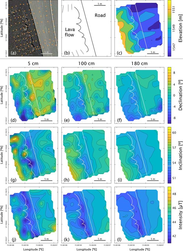
218                                                 B. M. de Groot and L. V. de Groot: Measuring local magnetic anomalies

and directions actually arise from local magnetic anomalies
caused by the magnetization of underlying lava flows. Local
anomalies are known to cause deviations in magnetic com-
pass readings in volcanic terrain, and they may therefore very
well influence the magnetic field as recorded by lavas when
they cool (Baag et al., 1995; Valet and Soler, 1999; Tanguy
and Le Goff, 2004).
    Here, we present a low-cost device that measures the am-
bient magnetic field at a selectable distance from the surface
of a lava flow to enable systematic mapping of local mag-
netic anomalies in volcanic terrain: the AnomalyMapper. Its
design revolves around a three-axis fluxgate sensor that is
mounted on an aluminum frame. To determine the declina-
tion, inclination, and intensity of the ambient magnetic field,
we need to know the orientation of the fluxgate sensor with
respect to true (geographic) north, east, and down. To this
end, there are two main hurdles to overcome: (1) it is impos-
sible to align the fluxgate sensor perfectly along the vertical
while measuring in volcanic terrain, and (2) we cannot use a        Figure 1. The AnomalyMapper. The AnomalyMapper consists of a
                                                                    GPS sensor, a tilt sensor, a fluxgate sensor, and a scope mounted on
magnetic compass to orient the fluxgate to true north, as we
                                                                    an aluminum frame, and it is operated by pressing buttons on a but-
are measuring local magnetic anomalies that interfere with          ton box (a). The electronic components are connected (red lines) to
compass readings. During normal operation it is possible to         a ruggedized laptop through USB interfaces, and the laptop has au-
keep the AnomalyMapper upright within ±3◦ of true verti-            dible feedback to the users. The AnomalyMapper is easily operated
cal by using a bubble level. To also correct for the remain-        by two people in the field (b), while the USB interface and laptop
ing deviation from vertical, we use an accelerometer (e.g.,         are carried in a small backpack.
tilt sensor) that is fixed to the fluxgate sensor to determine
the orientation of the AnomalyMapper with respect to the
direction of gravity; these measurements are used to rotate         sensor, interfaces between analog sensors and the laptop, and
the fluxgate measurements to true vertical. An intuitive way        all other hardware necessary to build the instrument.
to avoid using a magnetic compass would be to use a Sun
compass, but this would render the AnomalyMapper useless
                                                                    2     Physical description
when the sky is overcast. We therefore use a scope to orient
the AnomalyMapper to a fixed reference point on the ground          The backbone of the AnomalyMapper is a rectangular alu-
with a known (GPS) location. By logging the position of the         minum tube with dimensions 40 × 40 × 2000 mm (Fig. 1a).
AnomalyMapper for each measurement with a highly accu-              An aluminum I profile was glued along its entire length, al-
rate GPS sensor we can determine the bearing of the mea-            lowing the fluxgate sensor to slide from top to bottom us-
surement location to the reference point and hence rotate the       ing aluminum mounts (in which the stainless-steel bolts were
measurements to true north and east. This experimental de-          changed to brass ones). The tilt sensor was glued to the flux-
sign yields highly accurate magnetic measurements, while            gate sensor to ensure an assessment of the actual orientation
the measurements can be done quickly in the field.                  of the fluxgate sensor with respect to gravity. The GPS sensor
    To test the performance of the AnomalyMapper, we                was mounted at the top of the frame so that it is not obscured
mapped local magnetic anomalies nearby and on top of a              while the AnomalyMapper is in use. The scope (Lensolux 3–
block of lava from the 2002 flow of Mt. Etna (Sicily, Italy)        9 × 32, with crosshair) was fixed onto an aluminum profile
at three distances above the ground. Furthermore, we assess         and bolted to the frame using brass nuts, washers, and bolts.
the performance of the correction based on the tilt sensor to       About halfway along the frame a two-dimensional bubble
rotate the fluxgate measurements to true vertical during nor-       level was fixed to the frame using a small piece of aluminum
mal operation as well as under rather extreme circumstances         profile (Fig. 1a).
in which the AnomalyMapper was held under angles up to
25◦ from true vertical.                                             2.1    GPS sensor
    Our AnomalyMapper is a low-cost device, and many parts
are likely to be readily available in paleomagnetic labora-         The GPS sensor is a vital part of the AnomalyMapper as the
tories. Apart from the fluxgate sensor that is commercially         rotation towards true north and east depends on the accuracy
available for EUR ∼ 2000, the setup totals EUR < 1500, in-          of its known position. Here we use a commercially available
cluding a ruggedized laptop suitable for use in the field, a tilt   Navilock 6004P MD6 based on a u-blox NEO-6P chip set.
                                                                    It has a horizontal accuracy of < 1 m and a vertical accuracy

Geosci. Instrum. Method. Data Syst., 8, 217–225, 2019                   www.geosci-instrum-method-data-syst.net/8/217/2019/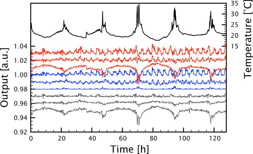
B. M. de Groot and L. V. de Groot: Measuring local magnetic anomalies                                                          219

of < 2 m. This sensor directly connects with the ruggedized        tances above the ground or to label repeated measurements
laptop through its USB interface. When starting a series of        at the same location. The button box is connected to digital
measurements the GPS sensor needs some time to acquire             inputs on the USB-1608G. A ruggedized Lenovo laptop runs
enough satellite fixes to provide an accurate location. This       the data collection software, requiring no user input in the
“cold start” is specified as 38 s but may be longer in prac-       field after initialization.
tice. During a series of measurements the GPS sensor is read
continuously to ensure that its reading is accurate 1 s after      2.5    Software
positioning the AnomalyMapper (hot start). During normal
operation this 1 s is needed to position and aim the Anoma-        The data collection software is written in LabVIEW 2017.
lyMapper to the reference point. The time needed to acquire        The software continuously collects GPS data and, when the
an accurate GPS position of the AnomalyMapper is therefore         operator presses a button, records data points for the fluxgate
not restrictive during normal use in the field.                    and tilt sensor. Data acquisition is simultaneous for all chan-
                                                                   nels at a 10 ksps sampling rate for 1000 samples per analog
2.2   Tilt sensor                                                  channel per measurement. The mean values of these 100 ms
                                                                   measurements are written into a .csv file along with the GPS
The orientation of the AnomalyMapper with respect to grav-         position for that measurement location and the height of the
ity is measured by a three-axis accelerometer chip; here we        measurement according to the button pressed. User feedback
choose an Analog Devices ADXL335 chip on a SparkFun                is an audible confirmation of a successful data point record-
breakout board (SEN-09269). The ADXL335 is a microelec-            ing or an audible warning when the GPS data are old or the
tromechanical system (MEMS) device with sensitivity corre-         fluxgate or tilt sensor data are outside expected bounds.
sponding to up to 0.1◦ , albeit with less than ideal drift char-
acteristics and offset as well as sensitivity accuracy that re-
quire calibration and correction. Offset and sensitivity cal-      3     Data acquisition
ibration values were established in the lab, and drift correc-
                                                                   The AnomalyMapper is easily operated by two people
tion values are calculated for each measurement session. This
                                                                   (Fig. 1b). The first aims the AnomalyMapper at the refer-
chip is powered from the laptop using a Seeed step-down
                                                                   ence point by looking through the scope, while the second
DC power converter based on an MP1584 chip from Mono-
                                                                   keeps the AnomalyMapper more or less upright by keeping
lithic Power Systems. The power supply voltage provided to
                                                                   an eye on the bubble level and acquires data by pushing the
the ADXL335 is measured simultaneously with each read-
                                                                   appropriate button on the button box. Aiming the Anoma-
out, as the three analog accelerometer outputs are ratiomet-
                                                                   lyMapper at the reference target needs to be done with great
ric to the power supply. Identical 1 Hz bandwidth resistor–
                                                                   care, as this orientation defines the measured declination of
capacitor (RC) low-pass filters are used on all four channels
                                                                   the magnetic field. If measurements are to be done at differ-
for increased noise reduction and accurate recording of the
                                                                   ent heights above the ground, it is easiest to use spray paint to
power supply voltage.
                                                                   indicate the measurement locations and follow the same sec-
2.3   Fluxgate sensor                                              tion as many times as necessary instead of moving the flux-
                                                                   gate along the frame of the AnomalyMapper multiple times
We used a commercially produced fluxgate sensor that was           per location.
readily available in our paleomagnetic laboratory: the Bart-
ington Mag-03MCES100 connected to a Bartington power
                                                                   4     Data processing and reference frames
supply and display unit. This fluxgate has a dynamic range
of 0 to 100 µT, which is well suited to measure the range of       The magnetic flux densities as measured by the fluxgate must
expected field intensities in volcanic terrain. It has a three-    be rotated towards north, east, and down to be informative
axis analog output, so the precision of the measurements is        on the full vector of the Earth’s magnetic field in a particular
determined by the analog–digital (AD) converter used; we           location. To this end four rotations are necessary: (1) align
chose a 16-bit AD converter, leading to an effective preci-        the tilt sensor measurements to the reference frame of the
sion of  25 nT.                                                   AnomalyMapper, (2) align the fluxgate measurements to the
                                                                   reference frame of the AnomalyMapper, (3) rotate the z axis
2.4   Interfacing and computer
                                                                   of the fluxgate measurements to vertical based on the tilt sen-
The analog outputs from the tilt and fluxgate sensors are con-     sor measurements while preserving the orientation of its x
nected to a USB data acquisition (DAQ) device; here we             axis to the direction of the reference point, and (4) rotate
used a Measurement Computing USB-1608G. In the field the           the measured magnetic flux densities towards north, east, and
main user interface is a handheld button box with four but-        down around the z axis of the AnomalyMapper.
tons. Each button gives a label (1–4) to the measured data, so
the four buttons can be used to measure at four different dis-

www.geosci-instrum-method-data-syst.net/8/217/2019/                    Geosci. Instrum. Method. Data Syst., 8, 217–225, 2019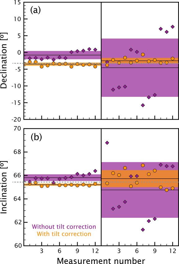
220 B. M. de Groot and L. V. de Groot: Measuring local magnetic anomalies
4.1 Aligning tilt sensor measurements to the 4.2 Aligning fluxgate measurements to the
AnomalyMapper’s frame AnomalyMapper’s frame
The tilt sensor is attached to the fluxgate such that gravity Although the fluxgate was carefully aligned to the frame of
during normal (upright) use is distributed over the three axes the AnomalyMapper, a small, fortuitous misalignment could
of the sensor so that each axis performs optimally. To rotate not be avoided. It is possible to rotate the fluxgate measure-
the tilt sensor measurements to the coordinate system as de- ments to the reference frame defined by the AnomalyMapper
fined by the frame of the AnomalyMapper (x in the direction using a similar rotation matrix as used for the tilt sensor, i.e.,
of the scope, y to the right of the scope, and z downwards by creating a matrix with fluxgate readouts while applying
along the rod; Fig. 2a), we define a rotation matrix. This ro- a magnetic field successively in the three orthogonal axes.
tation matrix is created with the readouts of the tilt sensor Since the z axis of the fluxgate is perfectly aligned with the z
when the AnomalyMapper is successively oriented with its x axis of the AnomalyMapper due to its construction, however,
(top row), y (middle row), and z (bottom row) axes aligned we choose to carefully measure the deviation of the x and y
with gravity. This yields the following rotation matrix for the axes of the fluxgate with respect to the coordinate system of
tilt sensor, Gf , in which the first character of the indices de- the AnomalyMapper (α, Fig. 2b) with a protractor and rotate
notes which axis of the AnomalyMapper was aligned with the fluxgate measurements around its z axis. This implies the
gravity and the second character indicates the axis of the tilt use of the following rotation matrix Bf ; due to the alignment
sensor: of the x, y, and z axes with respect to the AnomalyMapper
this rotation is in the negative direction (using an angle −α):
gxx gxy gxz
Gf = gyx gyy gyz .
cos(−α) − sin(−α) 0
gzx gzy gzz Bf = sin(−α) cos(−α) 0 .
0 0 1
The accuracy of the tilt sensor is affected by drift due to, e.g.,
temperature differences, but the precision within a limited The measured fluxgate data can now be rotated to the ref-
time span under constant conditions is very good (Sect. 2.2). erence frame of the AnomalyMapper by multiplying a mea-
To correct for this absolute drift between different sites and sured vector B m by this rotation matrix:
the moment the rotation matrix Gf was determined, we aver-
age all measurements done at one site (usually
100 mea- B f = B m · Bf .
surements) and assume that the average of these measure-
ments represents the true vertical, i.e., has the same orienta- 4.3 Putting the fluxgate measurements upright
tion as unit vector [001]. The vector of the averaged tilt sen-
sor measurements in its x, y, and z directions should there- While using the AnomalyMapper in the field great care is
fore be equal to the bottom row of Gf . Differences between taken to position the stick upright; since the AnomalyMapper
these two vectors arise from drift, and the measured data is handheld, however, deviations of up to ±3◦ are common.
should be corrected for this before rotation matrix Gf can With the data of the tilt sensor we can rotate the fluxgate data
be used to align the tilt sensor data to the reference frame de- to an upright reference frame with its z axis vertical (Fig. 2c–
fined by the AnomalyMapper. Hence we define a correction d), but we have to be careful to preserve the orientation of the
vector (1g) as the difference between the averaged measure- x axis of the AnomalyMapper towards the reference point. To
ments in the x, y, and z axes of the tilt sensor obtained at one this end we apply two rotations, the first around the x axis of
site (and within a couple of hours) and the bottom row of the new upright reference frame (φ) and the second around
rotation matrix Gf : its y axis (θ ). Due to the alignment of the x, y, and z axes
the rotation around the x axis is in the negative direction (us-
gx gzx ing an angle −φ), and the second is in the positive direction
1g = gy − gzy . (using an angle +θ ). The angles φ and θ are defined as
gz gzz
gy
φ = arctan
The tilt sensor data can now be rotated to the reference gz
frame of the AnomalyMapper by correcting a measured tilt and
vector (g m ) for drift and multiplying it by the inverse of the
rotation matrix: gx
θ = arctan ,
gz0
g = (g m − 1g) · G−1
f .
with gx , gy , and gz the tilt sensor data with respect to the
frame of the AnomalyMapper (i.e., vector g), and gz0 the
value of the z axis of the tilt sensor data after the rotation
Geosci. Instrum. Method. Data Syst., 8, 217–225, 2019 www.geosci-instrum-method-data-syst.net/8/217/2019/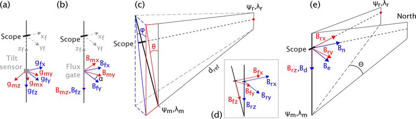
B. M. de Groot and L. V. de Groot: Measuring local magnetic anomalies 221
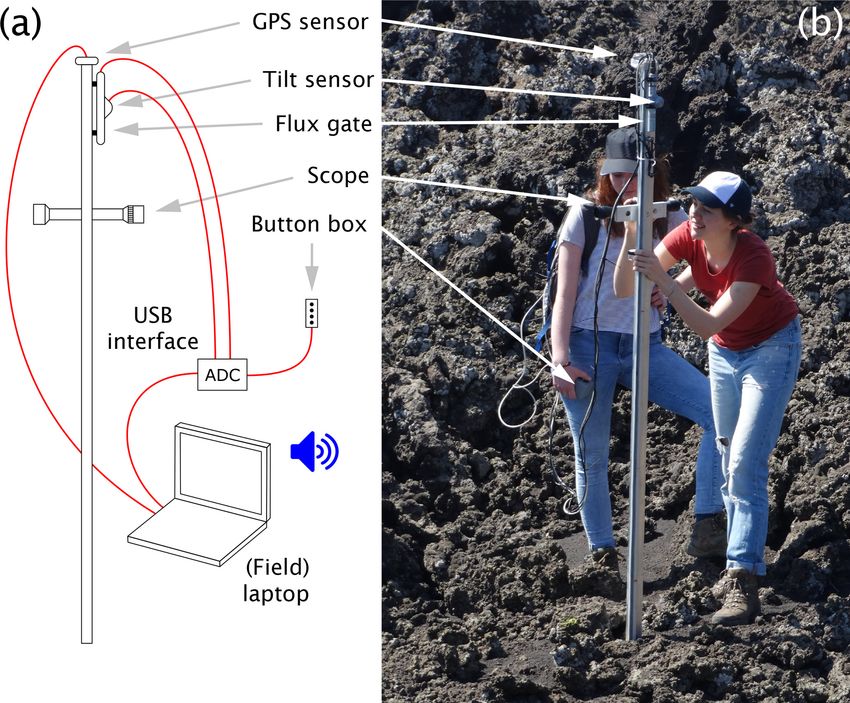
Figure 2. The different coordinate systems of the AnomalyMapper; in each panel the rotations are from the red to the blue coordinate
systems. The axes of the tilt sensor (gmx , gmy , gmz ) are rotated to the axes defined by the frame of the AnomalyMapper (gfx , gfy , gfz ) (a),
and the axes of the fluxgate (Bmx , Bmy , Bmz ) are rotated over angle α around the z axes of the AnomalyMapper to Bfx , Bfy , Bfz (b). Then
the tilt sensor measurements are used to rotate the fluxgate measurements in the system of the AnomalyMapper (Bfx , Bfy , Bfz ) over angles
φ and θ to the reference frame, with Brx pointing in the direction of the reference point (red dot; (9r , λr )); Bry and Brz are vertical (c, d).
The last rotation is over angle 2 (the bearing from the measurement location (9m , λm ) to the reference point) around the vertical axis to
align Brx to geographic north (Bn ) and Bry to geographic east (Be ) (e).
around the x axis of the new reference frame. The rotation To rotate the vector B r to geographic coordinates we de-
matrices associated with these rotations are fine the following rotation matrix to rotate over an angle −2
around the vertical axis,
1 0 0
R1 = 0 cos(−φ) − sin(−φ) cos(−2) − sin(−2) 0
0 sin(−φ) cos(−φ) R3 = sin(−2) cos(−2) 0 ,
0 0 1
and
cos(θ ) 0 sin(θ )
and multiply B r with this matrix:
R2 = 0 1 0 . B = B r · R3 .
− sin(θ ) 0 cos(θ )
To rotate the data to the reference system defined by the 5 Experimental results
reference point and the vertical a multiplication of vector B f
with the two rotation matrices is sufficient: To assess the performance of the AnomalyMapper we
mapped magnetic anomalies on a roadcut in the 2002 flow
B r = B f · R1 · R2 .
of Mt. Etna (15.7957◦ N, 15.0620◦ E). The anomalies were
4.4 Rotating fluxgate measurements towards true measured at 5, 100, and 180 cm above the ground, and we
north used a traffic sign approximately 200 m down the road as a
reference point. We measured a grid of 10 × 11 points in a
The final step of the data processing is to rotate the fluxgate rectangle of approximately 20×22 m. The road and rock face
data to true north using the locations of the reference point are roughly north–south. In each east–west line, the eastern-
and the AnomalyMapper (Fig. 2e). To this end we have to de- most four data points are on the road, then two or three points
termine the bearing (2) from the measurement location (i.e., are next to the rock face, and the remaining four to five points
the location of the AnomalyMapper) to the reference point are on top of the outcrop (Fig. 3a, b). The elevation was mea-
based on their GPS locations. Here we define the following: sured by the GPS sensor; although the accuracy of the GPS
ψm and λm are the latitude and longitude of the measurement sensor (vertically < 2 m) does not necessarily allow for the
location, and ψr and λr are the latitude and longitude of the mapping of the elevation of the outcrop properly, the main
reference point. The bearing from the location of the mea- structures are produced very well (Fig. 3c).
surement to the reference point with respect to true north is The local variations in declination, inclination, and inten-
then given by sity are mapped in contour plots. The local anomalies are
much more prominent at 5 cm above the ground and become
2 = arctan smoother at 100 and 180 cm above the ground (Fig. 3). The
sin (λr − λm ) · cos (ψr ) magnetic field is more homogenous above the road, although
.
cos (ψm ) · sin (ψr ) − sin (ψm ) · cos (ψr ) · cos (λr − λm ) the road is built on volcanic rock as well. Some features of
the magnetic field correlate closely with the topography of
www.geosci-instrum-method-data-syst.net/8/217/2019/ Geosci. Instrum. Method. Data Syst., 8, 217–225, 2019222 B. M. de Groot and L. V. de Groot: Measuring local magnetic anomalies Figure 3. Experimental results as acquired on a roadcut in the 2002 flow of Mt. Etna. The GPS locations of the measurements are orange dots on a Google Earth image (a). The road, rock face (wavy solid line), and shallower north and south slopes of the lava flow (dashed lines) are sketched (b); the rock face and edge of the road are indicated in white in the other panels. The elevation was determined by the GPS sensor (c). The declinations (d–f), inclinations (g–i), and intensities (j–l) were measured at 5 (d, g, j), 100 (e, h, k), and 180 cm (f, i, l) above the ground. For ease of comparison between panels with the same parameter the color schemes and contour lines are kept constant. The declination, inclination, and intensity as predicted by the International Geomagnetic Reference Field (IGRF, April 2018) are indicated as solid white lines in the scale bars. Geosci. Instrum. Method. Data Syst., 8, 217–225, 2019 www.geosci-instrum-method-data-syst.net/8/217/2019/
B. M. de Groot and L. V. de Groot: Measuring local magnetic anomalies                                                              223

the rock face, e.g., the positive (37.79567◦ N, 15.06193◦ E)
and negative (37.79563◦ N, 15.06195◦ E) anomalies in incli-
nation at 5 cm above the ground (Fig. 3g) and the low intensi-
ties at 100 cm above the ground at 37.79563◦ N, 15.06195◦ E
(Fig. 3k). Other anomalies at 5 cm above the ground may also
be due to the influence of loose boulders or rocks on top of
the lava flow that were easily > 30 cm in diameter (Fig. 3d,
g, j).

6     Discussion

6.1    Experience in the field

The AnomalyMapper is portable, suitable for air travel, and
easy to use in the field. The acquisition of all data in Fig. 3
took less than 2.5 h. Most parts of the AnomalyMapper are
(or can be built as) water resistant, so with proper precautions
to protect the ruggedized laptop and the I/O device against
rain it is possible to use the AnomalyMapper in most weather
conditions.
   The AnomalyMapper is most efficiently operated with two         Figure 4. Comparison of the declination (a) and inclination (b) be-
people: one aiming the AnomalyMapper at the reference              fore and after tilt correction. We did 12 measurements while care-
point, while the other keeps the AnomalyMapper more or             fully positioning the AnomalyMapper upright using the bubble level
                                                                   (deviation form vertical < 3◦ , left-hand side of both panels) and 12
less upright by looking at the bubble level. When the mag-
                                                                   measurements with the AnomalyMapper more or less upright (devi-
netic anomalies are to be measured at more than one height
                                                                   ation form vertical up to 25◦ , right-hand side of both panels). Each
above the ground it is most efficient to use spray paint to        measurement is plotted with (orange circles) and without (purple di-
mark the measurement locations and return to these points          amonds) tilt correction; the averages of groups of 12 measurements
after adjusting the height of the fluxgate.                        are given as horizontal black lines with their associated 1 standard
                                                                   deviation intervals as shading in the corresponding color. The gray
6.2    Accuracy and performance                                    dashed lines are the independently measured values of the Earth’s
                                                                   magnetic field.
The tilt sensor is an important part of the design of the
AnomalyMapper, as it enables accurate measurements when
the AnomalyMapper is not exactly aligned with true verti-
cal. To assess the performance of the tilt sensor we did 12        the declination and inclination are only 0.3◦ off the refer-
measurements in front of the paleomagnetic laboratory Fort         ence values. It must be emphasized that the reference val-
Hoofddijk at Utrecht University (52.08808◦ N, 5.17016◦ E)          ues were measured 1 year later, and slight deviations may
and processed the data with and without the tilt sensor cor-       be explained by changes in the ambient field, changes in the
rection in the spring of 2018. In June 2019, we obtained a         Earth’s magnetic field, or anthropogene contributions to the
reference measurement of the Earth’s magnetic field at the         ambient magnetic field.
same location using a horizontal surface that had an accuracy         We then repeated the 12 measurements but allowed the
of 0.03◦ . The obtained reference values for the declination,      AnomalyMapper to deviate up to 25◦ from true vertical
inclination, and intensity were −3.3◦ , 65.5◦ , and 47.9 µT, re-   (Fig. 4a and b, right). Before tilt correction this yielded
spectively. Since the intensity measurements are not affected      an average declination of −4.6 ± 8.7 and an inclination of
by the position of the AnomalyMapper we can compare the            64.6±2.4◦ . After correction using the tilt sensor data the dec-
averaged measured intensities with their 1 standard deviation      lination and inclination became −2.5 ± 0.8 and 65.7 ± 0.7◦ ,
(48.1 ± 0.03 µT) directly to the reference field: the measured     respectively. Again, the tilt sensor corrects the obtained de-
intensity is very close to the intensity value measured 1 year     clinations and inclinations to values closer to the reference
later but slightly higher.                                         measurement and, more importantly, to values closer to those
   During normal operation the AnomalyMapper can be kept           obtained by keeping the AnomalyMapper < 3◦ of true verti-
within < 3◦ of true vertical using the bubble level (Fig. 4a       cal. The deviations from the reference field are 0.8◦ for the
and b, left). Before tilt correction the declination (with its     declination and 0.2◦ for the inclination.
1 standard deviation) is −0.8 ± 1.2◦ and the inclination is           It is reassuring to note that the tilt sensor correction re-
65.8 ± 0.3◦ . After tilt correction the declination and inclina-   duces the standard deviation associated with the declina-
tion become −3.6 ± 0.5 and 65.2 ± 0.1◦ , respectively. Both        tions and inclinations dramatically; this implies that the mea-

www.geosci-instrum-method-data-syst.net/8/217/2019/                   Geosci. Instrum. Method. Data Syst., 8, 217–225, 2019
224 B. M. de Groot and L. V. de Groot: Measuring local magnetic anomalies
sured values converge towards their mean after tilt correc-
tion. Moreover, the declinations and inclinations for the mea-
surements done with the AnomalyMapper are within < 3◦
with deviations up to 25◦ ; these are pretty close, further tes-
tifying to the improvements in accuracy using the tilt sensor.
6.3 Temperature dependence of electronic components
The performance of the electronic parts of the AnomalyMap-
per is temperature dependent, and it is therefore important
to consider the temperature coefficients of the GPS, fluxgate,
tilt sensor, and DAQ devices. The Navilock 6004P MD6 GPS
Figure 5. Temperature dependance of the tilt sensor readings. The
sensor is built for outdoor use; its operating range is spec- temperature (in black) and the outputs of the ADXL335 (in red) and
ified as −20 to 60 ◦ C. Since its data acquisition and signal ADXL354 (in blue) were logged for 128 h. The difference between
processing are done digitally its accuracy is not affected by a the two sensors is in gray. For plotting purposes the output of the
thermal coefficient. The Bartington Mag-03MCES100 flux- tilt sensors was normalized to the mean of the first 500 readings of
gate has a specified operating range from −40 to 70 ◦ C, and the respective axis and then shifted to 1.03, 1.02, and 1.01 for the
its temperature-dependent offset is < 0.1 nT ◦ C−1 . During ADLX335 x, y, and z axes; 1.00, 0.99, and 0.98 for the ADLX354
normal use the temperature variation will be < 10 ◦ C over x, y, and z axes; and 0.97, 0.96, and 0.95 for the difference between
a measurement series, so the maximum error introduced by the two sensors (x, y, and z axes), respectively.
the fluxgate sensor is 1 nT. For the Measurement Computing
USB-1608G DAQ a temperature coefficient is not provided,
and its performance is specified while operating at 25 ◦ C. The 6.4 Drift correction of tilt sensor
operational temperature range is between 0 and 70 ◦ C. This
Due to the thermal and possible mechanical drift of the
DAQ converts the signals of the fluxgate and tilt sensor with
ADXL335 tilt sensor as outlined above we cannot use the
16-bit precision, while 14-bit precision would suffice the pre-
tilt sensor data in absolute terms. But, since the drift is lim-
cision of 0.01 µT for the fluxgate and 0.1◦ for the tilt sensor.
ited over the course of a couple of hours and a small tem-
The temperature coefficient of the GPS, fluxgate, and DAQ
perature range, we can use the mean value of all the data
devices can therefore safely be ignored.
points in one measurement session to create an assumed true
The output of the ADXL335 tilt sensor, however, is af-
vertical vector for that measurement session. The assump-
fected by changes in temperature. We therefore tested the
tion here is that over the course of a measurement session
temperature dependance of this sensor using a superior tilt
the AnomalyMapper is on average held upright. The rotation
sensor, the ADXL354, which has a temperature sensor on
matrix from the true vertical vector initially established in the
board. We mounted these two chips together on a servo motor
lab to the assumed true vertical vector from the mean value
that rotated over 25◦ at 10 s intervals. After five movements
for each session is applied to all data points in that session,
the servo returned to its initial position. To mimic temper-
thus providing individual long-term drift correction for each
ature variations during normal use in the field as closely as
measurement session.
possible, we put this setup in a windowsill in our laboratory
and let it run for 128 h. During these 5 d the temperature of 6.5 Choosing the reference target
the ADXL354 chip varied between 17.5 and 35.6 ◦ C (Fig. 5).
It is evident that the z axis of the ADXL335 chip especially Choosing the proper reference target is paramount, and it is
suffers from changes in temperature, as its output varies be- important to choose a point that can be seen from all mea-
tween −2.6 and +0.8 % over 18.1 ◦ C. The performance of surement points. The GPS sensor that determines the loca-
the ADXL354 is superior to the chip that we used for the tion of the AnomalyMapper has an accuracy of < 1 m. With
AnomalyMapper and is therefore preferable for future ver- a target at a distance of 200 m, the maximum deviation in
sions. It must be noted, however, that the tilt sensor chip as GPS position in the least favorable direction leads to an error
used in the AnomalyMapper is encapsulated in a blob of sil- in the bearing between the measurement and reference point
icon putty. This material is a good thermal insulator and sup- locations of < 0.3◦ . Choosing the target even further away
presses short-term temperature influences on the chip, such at 1 km, for example, reduces this error to < 0.06◦ . In these
as cloudy or sunny spells, while measuring. Moreover, the calculations the GPS location of the reference point is con-
temperature is not expected to change more than a few de- sidered accurate, as this location can be measured multiple
grees Celsius during a series of measurements. times to improve the accuracy of the GPS location and can
often easily be verified by satellite imagery.
Geosci. Instrum. Method. Data Syst., 8, 217–225, 2019 www.geosci-instrum-method-data-syst.net/8/217/2019/B. M. de Groot and L. V. de Groot: Measuring local magnetic anomalies 225
7 Conclusions Review statement. This paper was edited by Luis Vazquez and re-
viewed by four anonymous referees.
The AnomalyMapper is an accurate, easy to use, and low-
cost device to measure local magnetic anomalies in vol-
canic terrain. Considering the reproducibility of the mea-
surements during normal operation and the uncertainties as- References
sociated with the different parts of the AnomalyMapper, it Baag, C., Helsley, C. E., Xu, S., and Lienert, B. R.: Deflection of
is capable of determining declinations and inclinations with paleomagnetic directions due to magnetization of the underlying
an accuracy of at least < 0.5◦ . Data acquisition is quick: a terrain, J. Geophys. Res.-Sol. Ea., 100, 10013–10027, 1995.
grid of 110 points can be measured at three heights above Biggin, A. J., Perrin, M., and Dekkers, M. J.: A reliable abso-
the ground within 2.5 h. By making use of a reference point lute palaeointensity determination obtained from a non-ideal
on the ground to align the coordinate system of the Anoma- recorder, Earth Planet. Sc. Lett., 257, 545–563, 2007.
lyMapper to true north, east, and down, as well as a tilt Castro, J. and Brown, L.: Shallow paleomagnetic directions from
sensor to rotate the fluxgate measurements to true vertical, historic lava flows, Hawaii, Geophys. Res. Lett., 14, 1203–1206,
the accuracy of the measurements is greatly improved. This 1987.
Coe, R. S., Jarboe, N. A., Le Goff, M., and Petersen, N.: Demise of
experimental design also allows the AnomalyMapper to be
the rapid-field-change hypothesis at Steens Mountain: The cru-
used in all kinds of weather, except for very dense fog. The cial role of continuous thermal demagnetization, Earth Planet.
AnomalyMapper can be built for EUR < 1500 if a commer- Sc. Lett., 400, 302–312, 2014.
cial fluxgate sensor is at hand; otherwise, the total cost is de Groot, L. V., Biggin, A. J., Dekkers, M. J., Langereis, C. G., and
EUR ∼ 3500 for the entire setup. Herrero-Bervera, E.: Rapid regional perturbations to the recent
global geomagnetic decay revealed by a new Hawaiian record,
Nat. Commun., 4, 2727, https://doi.org/10.1038/ncomms3727,
Data availability. Both the raw data as measured by the Anoma- 2013a.
lyMapper and the processed data of the experiment on Mt. Etna are de Groot, L. V., Mullender, T. A. T., and Dekkers, M. J.: An eval-
available in the Supplement to this paper. uation of the influence of the experimental cooling rate along
with other thermomagnetic effects to explain anomalously low
palaeointensities obtained for historic lavas of Mt Etna (Italy),
Supplement. The supplement related to this article is available on- Geophys. J. Int., 193, 1198–1215, 2013b.
line at: https://doi.org/10.5194/gi-8-217-2019-supplement. Greve, A., Hill, M., Turner, G., and Nilsson, A.: The geomagnetic
field intensity in New Zealand: Palaeointensities from holocene
lava flows of the tongariro Volcanic centre, Geophys. J. Int., 211,
Author contributions. BMdG designed and built the instrument 814–830, 2017.
with the help of LVdG. LVdG prepared the paper with contributions Nilsson, A., Holme, R., Korte, M., Suttie, N., and Hill, M.: Recon-
from BMdG. structing Holocene geomagnetic field variation: new methods,
models and implications, Geophys. J. Int., 198, 229–248, 2014.
Pavón-Carrasco, F. J., Osete, M. L., Torta, J. M., and De Santis, A.:
A geomagnetic field model for the Holocene based on archaeo-
Competing interests. The authors declare that they have no conflict
magnetic and lava flow data, Earth Planet. Sc. Lett., 388, 98–109,
of interest.
2014.
Tanguy, J.-C. and Le Goff, M.: Distortion of the geomagnetic field
in volcanic terrains: an experimental study of the Mount Etna
Acknowledgements. Wout Krijgsman, Maartje van den Biggelaar, stratovolcano, Phys. Earth Planet. In., 141, 59–70, 2004.
and Lynn Vogel helped acquire the data on Mt. Etna presented in Valet, J.-P. and Soler, V.: Magnetic anomalies of lava fields in
this paper; Lynn Vogel processed the data, for which she is grate- the Canary islands. Possible consequences for paleomagnetic
fully acknowledged. records, Phys. Earth Planet. In., 115, 109–118, 1999.
Financial support. This research has been supported by the Dutch
Research Council (Nederlandse Organisatie voor Wetenschappelijk
Onderzoek, NWO; grant no. VENI 863.15.003).
www.geosci-instrum-method-data-syst.net/8/217/2019/ Geosci. Instrum. Method. Data Syst., 8, 217–225, 2019You can also read