Memory Wrap: a Data-Efficient and Interpretable Extension to Image Classification Models
←
→
Page content transcription
If your browser does not render page correctly, please read the page content below
Memory Wrap: a Data-Efficient and Interpretable
                                               Extension to Image Classification Models

                                                            Biagio La Rosa∗                            Roberto Capobianco
                                                      Sapienza University of Rome                   Sapienza University of Rome
                                                      larosa@diag.uniroma1.it                                Sony AI
                                                                                                  capobianco@diag.uniroma1.it
arXiv:2106.01440v2 [cs.LG] 4 Jun 2021

                                                                                     Daniele Nardi
                                                                               Sapienza University of Rome
                                                                               nardi@diag.uniroma1.it

                                                                                        Abstract
                                                    Due to their black-box and data-hungry nature, deep learning techniques are not
                                                    yet widely adopted for real-world applications in critical domains, like healthcare
                                                    and justice. This paper presents Memory Wrap, a plug-and-play extension to
                                                    any image classification model. Memory Wrap improves both data-efficiency
                                                    and model interpretability, adopting a content-attention mechanism between the
                                                    input and some memories of past training samples. We show that Memory Wrap
                                                    outperforms standard classifiers when it learns from a limited set of data, and it
                                                    reaches comparable performance when it learns from the full dataset. We discuss
                                                    how its structure and content-attention mechanisms make predictions interpretable,
                                                    compared to standard classifiers. To this end, we both show a method to build
                                                    explanations by examples and counterfactuals, based on the memory content, and
                                                    how to exploit them to get insights about its decision process. We test our approach
                                                    on image classification tasks using several architectures on three different datasets,
                                                    namely CIFAR10, SVHN and CINIC10.

                                        1       Introduction
                                        In the last decade, Artificial Intelligence has seen an explosion of applications thanks to advancements
                                        in deep learning techniques. Despite their success, these techniques suffer from some important
                                        problems: they require a lot of data to work well, and they act as black boxes, taking an input and
                                        returning an output without providing any explanation about that decision. The lack of transparency
                                        limits the adoption of deep learning in important domains like health-care and justice, while the data
                                        requirement makes harder its generalization on real-world tasks. Few-shot learning methods and
                                        explainable artificial intelligence (XAI) approaches address these problems. The former studies the
                                        data requirement, experimenting on a type of machine learning problem where the model can only
                                        use a limited number of samples; the latter studies the problem of transparency, aiming at developing
                                        methods that can explain, at least partially, the decision process of neural networks. While there is
                                        an extensive literature on each topic, few works explore methods that can be used both on low data
                                        regime and that can provide explanations about their outputs.
                                        This paper makes a little step in both directions, proposing Memory Wrap, an approach that makes
                                        image classification models more data-efficient by providing, at the same time, a way to inspect their
                                        decision process. In classical settings of supervised learning, models use the training set only to
                                            ∗
                                                Contact Author

                                        Preprint. Under review.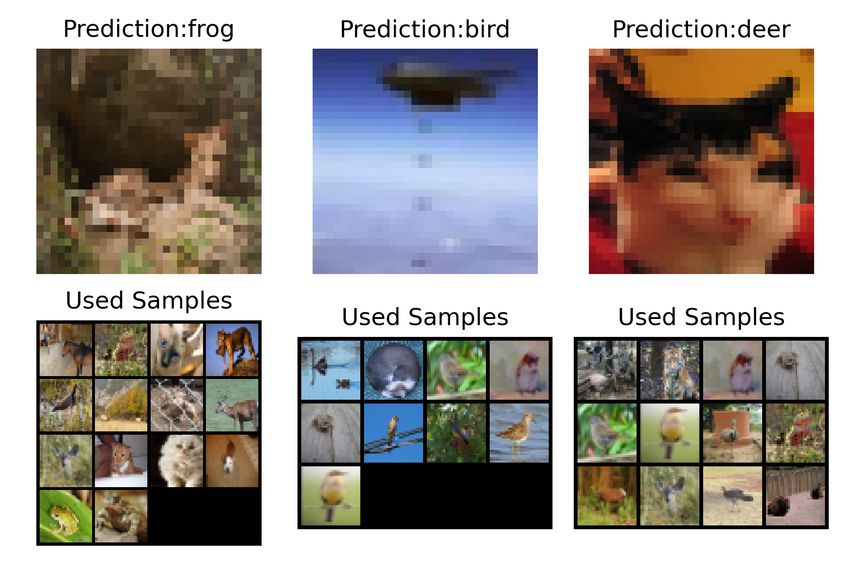
Prediction     7

                                                          Memory Wrap
                                            Encoder
                            Input
                                                                          Example

                                                                        Counterfactual
                          memory set

Figure 1: Overview of Memory Wrap. The encoder takes as input an image and a memory set, con-
taining random samples extracted from the training set. The encoder sends their latent representations
to Memory Wrap, which outputs the prediction, an explanation by example, and a counterfactual,
exploiting the sparse content attention between inputs encodings.

adjust their weights, discarding it at the end of the training process. Instead, we hypothesize that,
in a low data regime, it is possible to strengthen the learning process by re-using samples from the
training set during inference. Taking inspiration from Memory Augmented Neural Networks [6, 25],
the idea is to store a bunch of past training samples (called memory set) and combine them with the
current input through sparse attention mechanisms to help the neural network decision process. Since
the network actively uses these samples during inference, we propose a method based on inspection
of sparse content attention weights to extract insights and explanations about its predictions.
We test our approach on image classification tasks using CIFAR10 [13], Street View House Number
(SVHN) [21], and CINIC10 [4] obtaining promising results. Our contribution can be summarized as
follows:

       • we present Memory Wrap, an extension for image classification models that uses a memory
         containing past training examples to enrich the input encoding;
       • we show it makes the original model more data-efficient, achieving higher accuracy on low
         data regimes;
       • we discuss methods to make their predictions more interpretable. In particular, we show that
         not only it is possible to extract the samples that actively contribute to the prediction, but we
         can also measure how much they contribute. Additionally, we show a method to retrieve
         similar examples from the memory that allow us to inspect which features are important for
         the current prediction, in the form of explanation by examples and counterfactuals.

The manuscript is organized as follows. Section 2 reviews existing literature, focusing on works
that use similar methods to us and discuss the state-of-the-art in network explainability; Section 3
introduces our approach, while Section 4 presents some experiments and their results. Finally, we
discuss conclusions, limitations and future directions.

2     Background
2.1   Memory Augmented Neural Networks

Our work has been inspired by current advances in Memory Augmented Neural Networks
(MANNs) [6, 7, 14, 25]. MANNs use an external memory to store and retrieve data during in-
put processing. They can store past steps of a sequence, as in the case of recurrent architectures for
sequential tasks, or they can store external knowledge in form of a knowledge base [5]. Usually,
the network interacts with the memory through attention mechanisms, and it can also learn how to
write and read the memory during the training process [6]. Differentiable Neural Computers [7] and
End-To-End Memory Networks [25] are popular examples of this class of architectures. Researchers
apply them to several problems like visual question answering [19], image classification [2], and
meta-learning [23], reaching great results.
Similarly to MANNs, Matching Networks [29] use a set of never seen before samples to boost the
learning process of a new class in one-shot classification tasks. Differently from us, their architecture
is standalone and it applies the product of attention mechanisms on the labels of the sample set
in order to compute the final prediction. Conversely, Prototypical Networks [24] use samples of

                                                      2
the training set to perform metric learning and to return predictions based on the distance between
prototypes in the embedding space and the current input. Our approach relies on similar ideas, but
it uses a memory set that contains already seen and already learned examples in conjunction with
a sparse attention mechanism. While we adopt a similarity measure to implement our attention
mechanism, we do not use prototypes or learned distances: the network itself learns to choose which
features should be retrieved from each sample and which samples are important for a given input.
Moreover, our method differs from Prototype Networks because it is model agnostic and can be
potentially applied to any image classification model without modifications.

2.2   Explainable Artificial Intelligence

Lipton [16] distinguishes between transparent models, where one can unfold the chain of reasoning
(e.g. decision trees), and post-hoc explanations, that explain predictions without looking inside the
neural network. The last category includes explanation by examples and counterfactuals, which are
the focus of our method.
Explanations by examples aim at extracting representative instances from given data to show how
the network works [1]. Ideally, the instances should be similar to the input and, in classification
settings, predicted in the same class. In this way, by comparing the input and the examples, a human
can extract both similarities between them and features that the network uses to return answers.
Counterfactuals are specular to explanations by examples: the instances, in this case, should be
similar to the current input but classified in another class. By comparing the input to counterfactuals,
it is possible to highlight differences and to extract edits that should be applied to the current input to
obtain a different prediction. While for tabular data it is feasible to get counterfactuals by changing
features and at the same time to respect domain constraints [20], for images and natural language
processing the task is more challenging. This is due to the lack of formal constraints and to the
extremely large range of features to be changed.
Recent research on explanation by examples and counterfactuals adopts search methods [30, 18],
which have high latency due to the large search space, and Generative Adversarial Networks (GANs).
For example, Liu et al. [17] use GANs to generate counterfactuals for images, but – since they
are black-boxes themselves – it is difficult to understand why a particular counterfactual is a good
candidate or not.
For small problems, techniques like KNN and SVM [3] can easily compute neighbors of the current
input based on distance measures, and use them as example-based explanations. Unfortunately, for
problems involving a large number of features and neural networks, it becomes less trivial to find
a correct distance metric that both takes into account the different feature importance and that is
effectively linked to the neural network decision process. An attempt in this direction is the twin-
system proposed by Kenny and Keane [11], which combines case-based reasoning systems (CBR)
and neural networks. The idea is to map the latent space or neural weights to white-box case-based
reasoners and extract from them explanations by examples. With respect to these approaches, our
method is intrinsic, meaning that is embedded inside the architecture and, more importantly, it is
directly linked to the decision process, actively contributing to it. Our method does not require
external architectures like GANs or CBR and it does not have any latency associated with its use.

3     Memory Wrap

This section describes the architecture of Memory Wrap and a methodology to extract example-based
explanations and counterfactuals for its predictions.

3.1   Architecture

Memory Wrap extends existing classifiers, specialized in a given task, by replacing the last layer of
the model. Specifically, it includes a sparse content-attention mechanism and a multi-layer perceptron
that work together to exploit the combination of an input and a bunch of training samples. In this
way, the pre-existent model acts as an encoder, focused on extracting input features and mapping
them into a latent space. Memory Wrap stores previous examples (memories) that are then used at
inference time. The only requirement for the encoder is that its last layer – before the Memory Wrap

                                                    3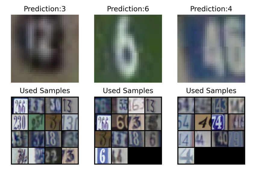
Memory Set                   Input

                                                  Encoder

                                      Encoding                Encoding
                                     memory set                 Input

                                                  Content
                                                  Attention

                                                  Memory
                                                  Vector                  Memory Wrap

                                                     +

                                                    MLP

                                                   Output

Figure 2: Sketch of the system architecture. The system encodes the input and a bunch of training
samples using a chosen neural network. Then, it generates a memory vector as a weighted sum of the
memory set based on the sparse content attention weights between the encodings. Finally, the last
layer predicts the input class, taking as input the concatenation of the memory vector and the input
encoding.

– outputs a vector containing a latent representation of the input. Clearly, the structure of the encoder
impacts on the representation power, so we expect that a better encoder architecture could improve
further the performance of Memory Wrap.
More formally, let be g(x) the whole model, f (x) the encoder, xi the current input, and Si =
{xim1 , xim2 , .., ximn } a set of n samples called memory set, randomly extracted from the training set
during the current step i. First of all, the encoder f (x) encodes both the input and the memory set,
projecting them in the latent space and returning respectively:
         exi = f (xi )          MSi = {mi1 , mi2 , .., min } = {f (xim1 ), f (xim2 ), .., f (ximn )}.   (1)
Then, Memory Wrap computes the sparse content attention weights as the sparsemax [22] of the
similarity between the input encoding and memory set encodings, thus attaching a content weight wj
to each encoded sample mij . We compute content attention weights using the cosine similarity as in
Graves et al. [7], replacing the sof tmax function with a sparsemax.

                               w = sparsemax(cosine[exi , MSi ]).                               (2)
Since we are using the sparsemax function, the memory vector only includes information from
few samples of the memory. In this way, each sample contributes in a significant way, helping us to
achieve output explainability. Similarly to [7], we compute the memory vector vSi as the weighted
sum of memory set encodings, where the weights are the content attention weights:
                                                  vSi = MTSi w.                                         (3)
 Finally, the last layer lf takes the concatenation of the memory vector and the encoded input, and
returns the final output
                                      oi = g(xi ) = lf ([e( xi ), vSi ]).                          (4)
The role of the memory vector is to enrich the input encoding with additional features extracted from
similar samples, possibly missing on the current input. On average, considering the whole memory
set and thanks to the cosine similarity, strong features of the target class will be more represented
than features of other classes, helping the network in the decision process. In our case, we use a
multi-layer perceptron with only one hidden layer as a final layer, but other choices are possible
(App. A.2).

3.2   Getting explanations

We aim at two types of explanations: explanation by examples and counterfactuals. The idea is
to exploit the memory vector and content attention weights to extract explanations about model

                                                              4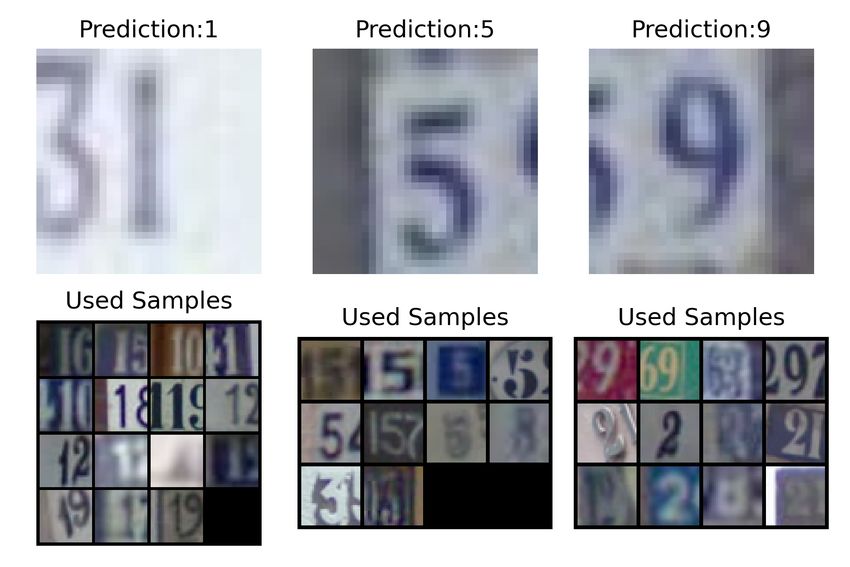
outputs, in a similar way to La Rosa et al. [15]. To understand how, let’s consider the current
input xi , the current prediction g(xi ), and the encoding matrix MSi of the memory set, where
each mij ∈ MSi is associated with a weight wj . We can split the matrix MSi into three disjoint
sets MSi = Me ∪ Mc ∪ Mz , where Me = {f (ximj ) | g(xi ) = g(ximj )} contains encodings of
samples predicted in the same class g(xi ) by the network and associated with a weight wj > 0,
Mc = {f (ximj ) | g(xi ) 6= g(ximj )} contains encodings of samples predicted in a different class and
associated with a weight wj > 0, and Mz contains encodings of samples associated with a weight
wj = 0. Note that this last set does not contribute at all to the decision process and it cannot be
considered for explainability purposes. Conversely, since Me and Mc have positive weights, they can
be used to extract explanation by examples and counterfactuals.
Let’s consider, for each set, the sample ximj associated with the highest weight. A high weight of wj
means that the encoding of the input xi and the encoding of the sample ximj are similar. If ximj ∈ Me ,
then it can be considered as a good candidate for an explanation by example, being an instance similar
to the input and predicted in the same class, as defined in Sect. 2.2. Instead, if ximj ∈ Mc , then it is
considered as a counterfactual, being similar to the input but predicted in a different class. Finally,
consider the sample ximk associated with the highest weight in the whole set MSi . Because it is
the highest, it will be heavily represented in the memory vector that will actively contribute to the
inference, being used as input for the last layer. This means that common features between the input
and the sample ximk are highly represented and so they constitute a good explanation. Moreover, if
ximk was a counterfactual, because it is partially included in the memory vector, it is likely that it will
be the second or third predicted class, giving also information about “doubts” of the neural network.

4     Results

This section first describes the experimental setups, and then it presents and analyzes the obtained
results for both performance and explanations.

4.1     Setup

We test our approach on image classification tasks using the Street View House Number (SVHN) [21],
CINIC10 [4] and CIFAR10 [13] datasets. For the encoder f (x), we run our tests using ResNet18 [8],
EfficientNet B0 [28], MobileNet-v2 [9], and other architectures whose results are reported in App. A.5.
We randomly split the training set to extract smaller sets in the range {1000,2000,5000}, thus
simulating a low regime data setting, and then train each model using these sets and the whole
dataset. At each training step, we randomly extract 100 samples from the training set and we use
them as memory set — ∼10 samples for each class (see App. A.7 and App. A.6 for further details
about this choice). We run 15 experiments for each configuration, fixing the seeds for each run
and therefore training each model under identical conditions. We report the mean accuracy and the
standard deviation over the 15 runs for each model and dataset. For further details about the training
setup please consult App. A.1.

4.1.1    Baselines

Standard. This baseline is obtained with the classifiers f (x) without any modification and trained
in the same manner of Memory Wrap (i.e. same settings and seeds).

Only Memory. This baseline uses only the memory vector as input of the multi-layer perceptron,
removing the concatenation with the encoded input. Therefore, the output is given by oi = g(xi ) =
lf (vSi ). In this case, the input is used only to compute the content weights, which are then used
to build the memory vector, and the network learns to predict the correct answer based on them.
Because of the randomness of the memory set and the absence of the encoded input image as input of
the last layer, the network is encouraged to learn more general patterns and not to exploit specific
features of the given image.

                                                    5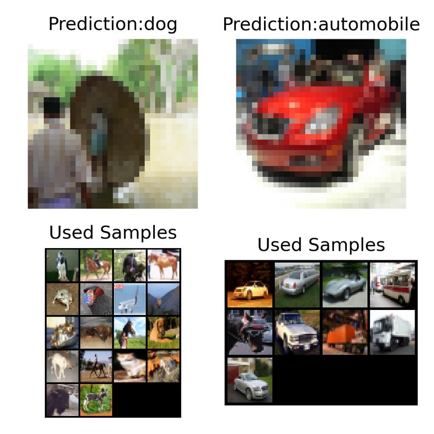
Table 1: Avg. accuracy and standard deviation over 15 runs of the baselines and Memory Wrap, when
the training dataset is a subset of SVHN. For each configuration, we highlight in bold the best result
and results that are within its margin.

                                Reduced SVHN Avg. Accuracy%
                                                                 Samples
                Model             Variant              1000           2000                5000
       EfficientNetB0          Standard        57.70 ± 7.89    72.59 ± 4.00      81.89 ± 3.37
                          Only Memory          58.86 ± 3.30    75.79 ± 1.68      85.30 ± 0.52
                          Memory Wrap          66.78 ± 1.27    77.37 ± 1.25      85.55 ± 0.59
        MobileNet-v2           Standard       42.71 ± 10.31    70.87 ± 4.20      85.52 ± 1.16
                          Only Memory          60.60 ± 3.14    80.80 ± 2.05      88.77 ± 0.42
                          Memory Wrap          66.93 ± 3.15    81.44 ± 0.76      88.68 ± 0.46
             ResNet18          Standard        20.63 ± 2.85   31.84 ± 18.38     79.03 ± 12.89
                          Only Memory          35.57 ± 6.48    68.87 ± 8.70      87.63 ± 0.42
                          Memory Wrap          45.31 ± 8.19    77.26 ± 3.38      87.74 ± 0.35

Table 2: Avg. accuracy and standard deviation over 15 runs of the baselines and Memory Wrap, when
the training dataset is a subset of CIFAR10. For each configuration, we highlight in bold the best
result and results that are within its margin.

                               Reduced CIFAR10 Avg. Accuracy%
                                                                 Samples
                  Model             Variant            1000          2000               5000
         EfficientNetB0          Standard      39.63 ± 2.16    47.25 ± 2.22    67.34 ± 2.37
                            Only Memory        40.60 ± 2.04    52.87 ± 2.07    70.82 ± 0.52
                            Memory Wrap        41.45 ± 0.79    52.83 ± 1.41    70.46 ± 0.78
          MobileNet-v2           Standard      38.57 ± 2.11    50.36 ± 2.64    72.77 ± 2.21
                            Only Memory        43.15 ± 1.35    57.43 ± 1.45    75.56 ± 0.76
                            Memory Wrap        43.87 ± 1.40    57.12 ± 1.36    75.33 ± 0.62
               ResNet18          Standard      40.03 ± 1.36    48.86 ± 1.57    65.95 ± 1.77
                            Only Memory        40.35 ± 0.89    51.11 ± 1.22    70.28 ± 0.80
                            Memory Wrap        40.91 ± 1.25    51.11 ± 1.13    69.87 ± 0.72

Table 3: Avg. accuracy and standard deviation over 15 runs on SVHN dataset of the baselines and
Memory Wrap. The comparison highlights the difference in performance when using a subset of the
dataset in the range {1k,2k,5k} as training set. For each configuration, we highlight in bold the best
result and results that are within its margin.

                               Reduced CINIC10 Avg. Accuracy%
                                                                 Samples
                  Model             Variant            1000          2000               5000
         EfficientNetB0          Standard      29.50 ± 1.18    33.56 ± 1.26    45.98 ± 1.34
                            Only Memory        30.46 ± 1.17    36.17 ± 1.54    44.97 ± 0.95
                            Memory Wrap        30.45 ± 0.64    36.65 ± 1.03    47.06 ± 0.91
          MobileNet-v2           Standard      29.61 ± 0.89    36.40 ± 1.58    50.41 ± 1.01
                            Only Memory        32.46 ± 1.07    39.91 ± 0.82    52.51 ± 0.77
                            Memory Wrap        32.34 ± 0.95    39.48 ± 1.16    52.18 ± 0.66
               ResNet18          Standard      31.18 ± 1.21    37.67 ± 0.98    45.39 ± 1.07
                            Only Memory        30.79 ± 0.83    37.30 ± 0.57    46.66 ± 0.81
                            Memory Wrap        32.15 ± 0.68    38.51 ± 0.96    46.39 ± 0.67

                                                   6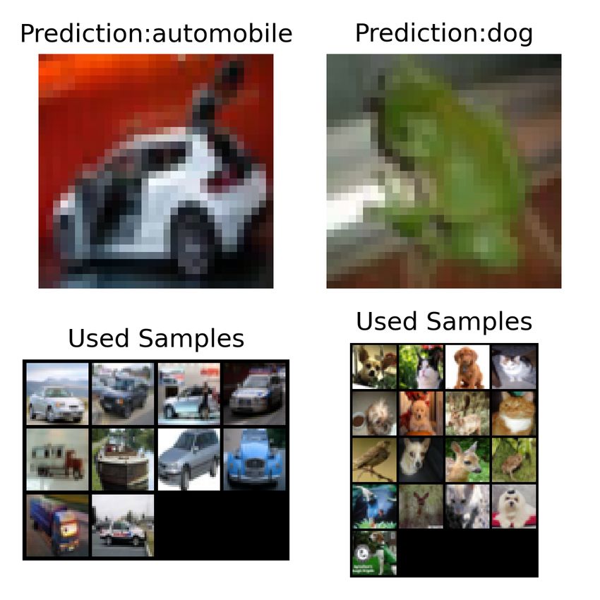
4.2 Performance
In low data regimes, our method outperforms the standard models in all the datasets, sometimes
with a large margin (Table 1, Table 3, and Table 2). First, we can observe that the amount of gain in
performance depends on the used encoder: MobileNet shows the largest gap in all the datasets, while
ResNet shows the smallest one, representing a challenging model for Memory Wrap. Secondly, it
depends on the dataset, being the gains in each SVHN configuration always greater than the ones
in CIFAR10 and CINIC10. Regarding the baseline that uses only the memory, it outperforms the
standard baseline too, reaching nearly the same performance of Memory Wrap in most of the settings.
However, its performance appears less stable across configurations, being lower than Memory Wrap
in some SVHN and CINIC10 settings (Table 1 and Table 3) and lower than standard models in some
full dataset scenarios and in some configurations of CINIC10. These considerations are confirmed
also on other architectures reported in App. A.5. We hypothesize that the additional information
captured by the input encoding allow the model to exploit additional shortcuts and to reach the best
performance.
Note that it is possible to increase the gap by adding more samples in the memory, at the cost of
an increased training and inference time (App. A.7). Moreover, while in low data regimes standard
neural networks performances show high variance, Memory Wrap seems to be a lot more stable with
a lower standard deviation.
When Memory Wrap learns from the full dataset (Table 4), it reaches comparable performance
most of the time. Hence, our approach is useful also when used with the full dataset, thanks to the
additional interpretability opportunity provided by its structure (Section 3.2).
4.3 Explanations
From now on, we will consider MobileNet-v2 as our base network, but the results are similar for
all the considered models and configurations (App. A.4 and A.8). The first step that we can do to
extract insights about the decision process, is to check which samples in the memory set have positive
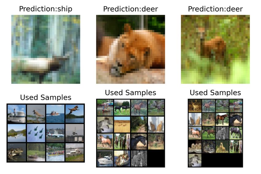
weights – the set Mc ∪ Me . Figure 3 shows this set ordered by the magnitude of content weights for
four different inputs: each couple shares the same memory set as additional input, but each set of used
samples – those associated with a positive weight – is different. In particular, consider the images in
Figure 3a, where the only change is a lateral shift made to center different numbers. Despite their
closeness in the input space, samples in memory are totally different: the first set contains images of
“5” and “3”, while the second set contains mainly images of “1” and few images of “7”. We can infer
that probably the network is focusing on the shape of the number in the center to classify the image,
ignoring colors and the surrounding context. Conversely, in Figure 3b the top samples in memory are
images with similar colors and different shapes, telling us that the network is wrongly focusing on
the association between color in the background and color of the object in the center. This means that
the inspection of samples in the set Mc ∪ Me can give us some insights about the decision process.
Table 4: Avg. accuracy and standard deviation over 15 runs of the baselines and Memory Wrap,
when the training datasets are the whole SVHN and CIFAR10 datasets. For each configuration, we
highlight in bold the best result and results that are within its margin.
Full Datasets Avg. Accuracy %
Model Variant SVHN CIFAR10 CINIC10
EfficientNetB0 Standard 94.39 ± 0.24 88.13 ± 0.38 77.31 ± 0.35
Only Memory 94.63 ± 0.33 86.48 ± 0.29 76.19 ± 0.25
Memory Wrap 94.67 ± 0.16 88.05 ± 0.20 77.34 ± 0.27
MobileNet-v2 Standard 95.95 ± 0.09 88.78 ± 0.41 78.97 ± 0.31
Only Memory 95.59 ± 0.11 86.37 ± 0.21 74.60 ± 0.13
Memory Wrap 95.63 ± 0.08 88.49 ± 0.32 79.05 ± 0.15
ResNet18 Standard 95.79 ± 0.18 91.94 ± 0.19 82.05 ± 0.25
Only Memory 95.82 ± 0.10 91.36 ± 0.24 81.65 ± 0.19
Memory Wrap 95.58 ± 0.06 91.49 ± 0.17 82.04 ± 0.16
7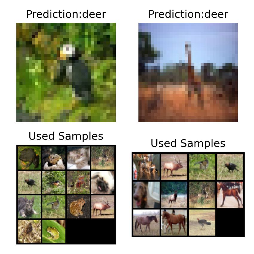
(a)                             (b)                              (c)

Figure 3: Inputs (first rows), their associated predictions and an overview of the samples in the
memory set that have an active influence on the decision process – i.e. the samples on which the
memory vector is built – (second row).

Once we have defined the nature of the samples in the memory set that influence the inference process,
we can check whether the content weight ranking is meaningful for Memory Wrap predictions. To
verify that this is the case, consider the most represented sample inside the memory vector (i.e. the
sample ximk associated with the highest content weight). Then, let g(ximk ) be the prediction obtained
by replacing the current input with this sample, and the current memory set Si with a new one. If

Table 5: Mean Explanation accuracy and standard deviation over 15 runs of the sample in the memory
set with the highest sparse content attention weight.
                                    Explanation Accuracy %
                         Dataset   Samples      Only Memory       Memory Wrap
                         SVHN          1000      81.46 ± 1.05       84.26 ± 1.29
                                       2000      89.53 ± 1.05       90.76 ± 0.50
                                       5000      93.79 ± 0.23       94.56 ± 0.20
                      CIFAR10          1000      77.81 ± 0.93       78.03 ± 0.81
                                       2000      82.39 ± 0.65       82.01 ± 0.49
                                       5000      89.17 ± 0.34       88.49 ± 0.26
                       CINIC10         1000      75.99 ± 0.80       76.30 ± 0.75
                                       2000      78.38 ± 0.46       78.43 ± 0.55
                                       5000      80.90 ± 0.33       74.47 ± 0.62

Table 6: Accuracy reached by the model on images where the sample with the highest weight in
memory set is a counterfactual. The accuracy is computed as the mean over 15 runs using as encoder
MobileNet-v2.
                                         Accuracy %
                         Dataset    Samples     Only Memory      Memory Wrap
                          SVHN         1000      35.45 ± 2.47      39.90 ± 1.84
                                       2000      43.79 ± 1.20      45.60 ± 1.08
                                       5000      48.02 ± 1.02      49.02 ± 1.39
                       CIFAR10         1000      30.56 ± 1.08      31.78 ± 0.82
                                       2000      36.93 ± 0.83      37.15 ± 0.70
                                       5000      44.57 ± 1.19      45.80 ± 0.77
                       CINIC10         1000      25.20 ± 0.57      25.36 ± 0.62
                                       2000      28.77 ± 0.42      28.70 ± 0.59
                                       5000      34.18 ± 0.56      35.22 ± 0.46

                                                     8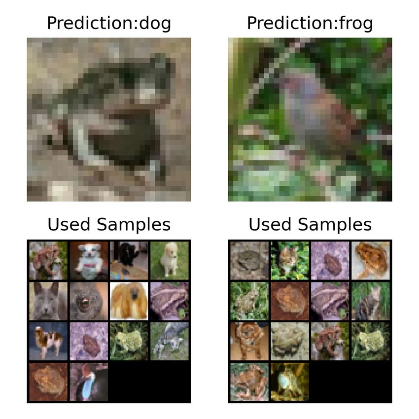
(a)                     (b)                   (c)                      (d)
Figure 4: Integrated Gradients heatmaps of the input, the explanation by example associated with the
highest weight in memory, and (eventually) the counterfactual associated with the highest weight.
Each heatmap highlights the pixels that have a positive impact towards the current prediction.

the sample influences in a significant way the decision process and if it can be considered as a good
proxy for the current prediction g(xi ) (i.e a good explanation by example), then g(ximk ) should be
equal to g(xi ). Therefore, we set the explanation accuracy as a measure that checks how many times
the sample in the memory set with the highest weight is predicted in the same class of the current
image. Table 5 shows the explanation accuracy of MobileNet-v2 in all the considered configurations.
We observe that Memory Wrap reaches high accuracy, meaning that the content weights ranking is
reliable. Additionally, its accuracy is very close to the baseline that uses only the memory, despite
the fact this latter is favored by its design, meaning that the memory content heavily influences the
decision process.
Clearly, the same test cannot be applied to counterfactuals, because, by construction, they are samples
of a different class. However, we can inspect what happens when a counterfactual is the sample with
the highest weight. We find (Table 6) that the model accuracy is much lower in these cases, meaning
that its predictions are often wrong and one can use this information to alert the user that the decision
process could be unreliable.
Since the memory is actively used during the inference phase, we can use attribution methods to
extract further insights about the decision process (see App. A.3 for a discussion about the choice
of the attribution method). For example, Figure 4 shows heatmaps obtained applying Integrated
Gradients2 [26], a method that highlights the most relevant pixels for the current prediction, exploiting
the gradients. For both Figure 4a and Figure 4d, the model predicts the wrong class. In the 4d case,
the heatmap of the explanation by example tells us that the model focuses on bird and sky colors,
ignoring the unusual shape of the airplane, very different from previously known shapes for airplanes,
which are represented by the counterfactual with a very low weight and a heatmap that focuses only
on the sky. Conversely in the 4c case, the model ignores colors and focuses on the head shape, a
feature that is highlighted both in the input image and in the explanations. Finally, sometimes (see
Figure 4b) counterfactuals are missing, and this means that the model is sure about its prediction and
it uses only examples of the same class.

5       Conclusion and future research
In this paper, we presented an extension for neural networks that allows a more efficient use of the
training dataset in settings where few data are available. Moreover, we propose an approach to extract
explanations based on similar examples and counterfactuals.
Future work could explore the reduction of current limitations, like the memory space needed to
store the memory samples and their gradients (App. A.6). Another limitation is that the memory
mechanism based on similarity could amplify the bias learned by the encoder. As shown in Sect. 3.2,
the identification of such an event is straightforward, but currently there are not countermeasures
    2
        We use the Captum library [12]

                                                   9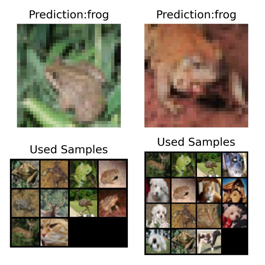
against it. A new adaptive or algorithmic selection mechanism of memory samples or a regularization
method could mitage the bias and it could improve the fairness of Memory Wrap. Finally, the findings
of this paper open up also possible extensions on different problems like semi-supervised learning,
where the self uncertainty detection of Memory Wrap could be useful, and domain adaption.

Acknowledgments and Disclosure of Funding
This material is based upon work supported by Google Cloud.

References
[1] Vaishak Belle and Ioannis Papantonis. Principles and practice of explainable machine learning.
   2020.
[2] Qi Cai, Yingwei Pan, Ting Yao, Chenggang Yan, and Tao Mei. Memory matching networks
   for one-shot image recognition. In 2018 IEEE/CVF Conference on Computer Vision and Pattern
   Recognition. IEEE, 2018.
[3] Corinna Cortes and Vladimir Vapnik. Support-vector networks. Machine Learning, 20(3):273–
   297, 1995.
[4] Luke N. Darlow, Elliot J. Crowley, Antreas Antoniou, and Amos J. Storkey. Cinic-10 is not
   imagenet or cifar-10. October 2018.
[5] Emily Dinan, Stephen Roller, Kurt Shuster, Angela Fan, Michael Auli, and Jason Weston. Wizard
   of wikipedia: Knowledge-powered conversational agents. 2018.
[6] Alex Graves, Greg Wayne, and Ivo Danihelka. Neural turing machines. 2014.
[7] Alex Graves, Greg Wayne, Malcolm Reynolds, Tim Harley, Ivo Danihelka, Agnieszka Grabska-
   Barwińska, Sergio Gómez Colmenarejo, Edward Grefenstette, Tiago Ramalho, John Agapiou,
   Adrià Puigdomènech Badia, Karl Moritz Hermann, Yori Zwols, Georg Ostrovski, Adam Cain,
   Helen King, Christopher Summerfield, Phil Blunsom, Koray Kavukcuoglu, and Demis Hassabis.
   Hybrid computing using a neural network with dynamic external memory. Nature, 538(7626):471–
   476, 2016.
[8] Kaiming He, Xiangyu Zhang, Shaoqing Ren, and Jian Sun. Deep residual learning for image
   recognition. In 2016 IEEE Conference on Computer Vision and Pattern Recognition (CVPR).
   IEEE, 2016.
[9] Andrew G. Howard, Menglong Zhu, Bo Chen, Dmitry Kalenichenko, Weijun Wang, Tobias
   Weyand, Marco Andreetto, and Hartwig Adam. Mobilenets: Efficient convolutional neural
   networks for mobile vision applications. 2017.
[10] Gao Huang, Zhuang Liu, Laurens Van Der Maaten, and Kilian Q. Weinberger. Densely
   connected convolutional networks. In 2017 IEEE Conference on Computer Vision and Pattern
   Recognition (CVPR). IEEE, 2017.
[11] Eoin M. Kenny and Mark T. Keane. Twin-systems to explain artificial neural networks using
   case-based reasoning: Comparative tests of feature-weighting methods in ANN-CBR twins for
   XAI. In Proceedings of the Twenty-Eighth International Joint Conference on Artificial Intelligence.
   International Joint Conferences on Artificial Intelligence Organization, 2019.
[12] Narine Kokhlikyan, Vivek Miglani, Miguel Martin, Edward Wang, Bilal Alsallakh, Jonathan
   Reynolds, Alexander Melnikov, Natalia Kliushkina, Carlos Araya, Siqi Yan, and Orion Reblitz-
   Richardson. Captum: A unified and generic model interpretability library for pytorch. 2020.
[13] A. Krizhevsky. Learning multiple layers of features from tiny images. 2009.
[14] Ankit Kumar, Ozan Irsoy, Peter Ondruska, Mohit Iyyer, James Bradbury, Ishaan Gulrajani, Vic-
   tor Zhong, Romain Paulus, and Richard Socher. Ask me anything: Dynamic memory networks for
   natural language processing. In Proceedings of the 33rd International Conference on International
   Conference on Machine Learning, volume 48 of ICML’16, page 1378–1387. JMLR.org, 2016.

                                                 10
[15] Biagio La Rosa, Roberto Capobianco, and Daniele Nardi. Explainable inference on sequential
data via memory-tracking. In Proceedings of the Twenty-Ninth International Joint Conference
on Artificial Intelligence. International Joint Conferences on Artificial Intelligence Organization,
2020.
[16] Zachary C. Lipton. The mythos of model interpretability: In machine learning, the concept of
interpretability is both important and slippery. Queue, 16(3):31–57, 2018.
[17] Shusen Liu, Bhavya Kailkhura, Donald Loveland, and Yong Han. Generative counterfactual
introspection for explainable deep learning. 2019.
[18] Arnaud Van Looveren and Janis Klaise. Interpretable counterfactual explanations guided by
prototypes. 2019.
[19] Chao Ma, Chunhua Shen, Anthony Dick, Qi Wu, Peng Wang, Anton van den Hengel, and
Ian Reid. Visual question answering with memory-augmented networks. In 2018 IEEE/CVF
Conference on Computer Vision and Pattern Recognition. IEEE, 2018.
[20] Divyat Mahajan, Chenhao Tan, and Amit Sharma. Preserving causal constraints in counterfactual
explanations for machine learning classifiers. 2019.
[21] Yuval Netzer, Tao Wang, Adam Coates, Alessandro Bissacco, Bo Wu, and Andrew Y. Ng.
Reading digits in natural images with unsupervised feature learning. In NIPS Workshop on Deep
Learning and Unsupervised Feature Learning 2011, 2011.
[22] Ben Peters, Vlad Niculae, and André F. T. Martins. Sparse sequence-to-sequence models.
In Proceedings of the 57th Annual Meeting of the Association for Computational Linguistics.
Association for Computational Linguistics, 2019.
[23] Adam Santoro, Sergey Bartunov, Matthew Botvinick, Daan Wierstra, and Timothy Lillicrap.
Meta-learning with memory-augmented neural networks. volume 48 of Proceedings of Machine
Learning Research, pages 1842–1850. PMLR, 2016.
[24] Jake Snell, Kevin Swersky, and Richard Zemel. Prototypical networks for few-shot learning.
In Proceedings of the 31st International Conference on Neural Information Processing Systems,
NIPS’17, page 4080–4090. Curran Associates Inc., 2017.
[25] Sainbayar Sukhbaatar, Arthur Szlam, Jason Weston, and Rob Fergus. End-to-end memory
networks. In Proceedings of the 28th International Conference on Neural Information Processing
Systems - Volume 2, NIPS’15, page 2440–2448. MIT Press, 2015.
[26] Mukund Sundararajan, Ankur Taly, and Qiqi Yan. Axiomatic attribution for deep networks. In
Proceedings of the 34th International Conference on Machine Learning - Volume 70, ICML’17,
page 3319–3328. JMLR.org, 2017.
[27] Christian Szegedy, Wei Liu, Yangqing Jia, Pierre Sermanet, Scott Reed, Dragomir Anguelov,
Dumitru Erhan, Vincent Vanhoucke, and Andrew Rabinovich. Going deeper with convolutions. In
Proceedings of the IEEE Conference on Computer Vision and Pattern Recognition (CVPR), June
2015.
[28] Mingxing Tan and Quoc Le. EfficientNet: Rethinking model scaling for convolutional neural
networks. volume 97 of Proceedings of Machine Learning Research, pages 6105–6114. PMLR,
2019.
[29] Oriol Vinyals, Charles Blundell, Timothy Lillicrap, Koray Kavukcuoglu, and Daan Wierstra.
Matching networks for one shot learning. In Proceedings of the 30th International Conference on
Neural Information Processing Systems, NIPS’16, page 3637–3645. Curran Associates Inc., 2016.
[30] Sandra Wachter, Brent Mittelstadt, and Chris Russell. Counterfactual explanations without
opening the black box: Automated decisions and the gdpr. Harvard Journal of Law and Technology,
31(2):841–887, 2018.
[31] Xiangyu Zhang, Xinyu Zhou, Mengxiao Lin, and Jian Sun. ShuffleNet: An extremely efficient
convolutional neural network for mobile devices. In 2018 IEEE/CVF Conference on Computer
Vision and Pattern Recognition. IEEE, jun 2018.
11A Appendix
A.1 Training Details
A.1.1 Datasets.
We test our approach on image classification tasks using the Street View House Number (SVHN)
dataset [21] (GNU 3.0 license), CINIC10 [4](MIT license) and CIFAR10 [13](MIT license). SVHN
is a dataset containing ∼73k images of house numbers in natural scenarios. The goal is to recognize
the right digit in the image. Sometimes some distracting digits are present next to the centered digits
of interest. CIFAR10 is an extensively studied dataset containing ∼60k images where each image
represents one of the 10 classes of the dataset. Finally, CINIC10 is relatively new dataset containing
∼90k images that tries to bridge the gap betwen CIFAR10 and ImageNet in terms of difficulty, using
the same classes of CIFAR10 and a subset of merged images from both CIFAR10 and ImageNet.
At the beginning of our experiments, we randomly extract from training sets a validation test of 6k
images for each dataset. The images are normalized and, in CIFAR10 and CINIC10, we also apply
an augmentation based on random horizontal flips. We do not use the random crop augmentation
because, in some preliminary tests, it can hurt the performance, as a random crop can often isolate a
portion of the image containing only the background. The memory in this case will retrieve similar
examples based only on the background, pushing the network to learn useless shortcuts, degrading
the performance.
The subsets of the training dataset to train models with 1000, 2000 and 5000 samples are extracted
randomly and change in every run. This means that we extract 15 different subsets of the dataset and
then test all the configurations on these subsets. We fixed the seed using the range (0,15) to make the
results reproducible.
A.1.2 Training details.
The implementation of the architectures for our encoders f (x) starts from the PyTorch implementa-
tions of Kuang Liu3 . To train the models, we follow the setup of Huang et al. [10], where they are
trained for 40 epochs in SVHN and 300 epochs in CIFAR10. In both cases, we apply the Stochastic
Gradient Descent (SGD) algorithm providing a learning rate that starts from 1e-1 and decreases by
a factor of 10 after 50% and 75% of epochs. Note that this configuration is not optimal neither for
baselines nor for Memory Wrap and you can reach higher performance on both cases by choosing
another set of hyperparameters tuned in each setting. However, this makes quite fair the comparison
across different models and datasets. We ran our experiment using a cloud hosted NVIDIA A100 and
a GTX 3090.
Memory Set Regarding memory samples, in an ideal setting one should provide a new memory set
for each input during the training process, however this makes both the training and the inference
process slowe due to computational limits. We simplified the process by providing a single memory
set for each new batch. The consequence is that performance at testing/validation time can be
influenced by the batch size used: a high batch size means a high dependency on the random selection.
To limit the instability, we fix a batch size at testing time of 500 and we repeat the test phase 5 times,
extracting the average accuracy across all repetitions.
A.2 Final Layer.
In this section, we describe and motivate the choice of the parameters of the last layer. In principle,
we can use any function as the last layer. In some preliminary tests, we compared a linear layer
against a multi-layer perceptron. We found that linear layers require lower learning rates (in the
range of [1e-2,1e-4]) to work well in our settings. However, for the considered datasets and models,
the standard configuration requires a decreasing learning rate that starts from high values. To
make the comparison fair, we choose, instead, a multi-layer perceptron that seems more stable and
reliable at high learning rates. The choice of a linear layer is appealing, because it makes easier
the inspection of the contribution of each sample in the memory to compute the final prediction,
and in principle, one could obtain similar or higher results if hyperparameters are suitably tuned.
3
https://github.com/kuangliu/pytorch-cifar
12We use a multi-layer perceptron containing only 1 hidden layer. The input dimension of such a
layer will be clearly dim(lf ) = 2dim(exi ) being dim(exi ) = dim(vSi ) for the Memory Wrap and
dim(lf ) = dim(vSi ), for the baseline that uses only the memory vector. The size of the hidden layer
dim(hlf ) is a hyper-parameter that we fix multiplying the input size by a factor of 2.
A.3 Attribution Methods.
As described in the paper, it is possible to use an attribution method to highlight the most important
pixels for both the input image and the memory set, with respect to the current prediction. The
only requirement is that the attribution method must support multi-input settings. We use the
implementation of Integrated Gradients [26] provided by the Captum library [12]. Note that, one of
the main problems of these attribution methods is the choice of the baseline [26]: it should represent
the absence of information. In the image domain, it is difficult to choose the right baseline, because
there is a high variability of shapes and colors. We selected a white image as the baseline, because it
is a common background on SVHN dataset, but this choice generates two effects: 1) it makes the
heatmaps blind to white color and this means, for example, that heatmaps for white numbers on a
black background focus on edges of numbers instead of the inner parts; 2) it is possible to obtain a
different heatmap by changing the baseline.
A.4 Explanation Accuracy.
Table 7 shows the complete set of experiments for the computation of the explanation accuracy.
Table 7: Mean Explanation accuracy and standard deviation over 15 runs of the sample in the memory
set with the highest sparse content attention weight.
Explanation Accuracy Memory Wrap %
Dataset Samples EfficientNetB0 ResNet18
SVHN 1000 86.09 ± 0.76 69.85 ± 3.29
2000 90.04 ± 0.51 84.64 ± 2.02
5000 93.19 ± 0.49 92.45 ± 0.26
CIFAR10 1000 80.06 ± 0.85 72.95 ± 1.00
2000 80.27 ± 0.57 78.42 ± 0.58
5000 85.05 ± 0.47 85.86 ± 0.46
13A.5 Additional Architectures.
Table 8 and Table 9 show the performance of GoogLeNet [27], DenseNet [10], and ShuffleNet [31]
on both datasets. We can observe that the performance trend follows that of the other architectures.
Table 8: Avg. accuracy and standard deviation over 15 runs of the baselines and Memory Wrap, when
the training dataset is a subset of SVHN. For each configuration, we highlight in bold the best result
and results that are within its margin.
Reduced SVHN Avg. Accuracy%
Samples
Model Variant 1000 2000 5000
GoogLeNet Standard 25.25 ± 9.39 61.45 ± 16.56 88.63 ± 2.60
Only Memory 66.35 ± 6.93 87.10 ± 1.17 92.16 ± 0.28
Memory Wrap 74.66 ± 9.01 88.32 ± 0.78 92.52 ± 0.25
DenseNet Standard 60.93 ± 9.21 83.47 ± 1.16 89.39 ± 0.60
Only Memory 40.94 ± 12.06 79.12 ± 5.36 89.69 ± 0.63
Memory Wrap 73.69 ± 4.20 85.12 ± 0.62 90.07 ± 0.49
ShuffleNet Standard 27.09 ± 6.05 60.05 ± 8.76 83.19 ± 1.00
Only Memory 32.22 ± 3.47 60.06 ± 3.32 85.56 ± 0.60
Memory Wrap 33.60 ± 4.69 67.35 ± 3.19 85.04 ± 0.74
Table 9: Avg. accuracy and standard deviation over 15 runs of the baselines and Memory Wrap, when
the training dataset is a subset of CIFAR10. For each configuration, we highlight in bold the best
result and results that are within its margin.
Reduced CIFAR10 Avg. Accuracy%
Samples
Model Variant 1000 2000 5000
GoogLeNet Standard 51.91 ± 3.14 63.90 ± 2.21 79.09 ± 1.28
Only Memory 54.25 ± 0.80 66.00 ± 1.27 79.65 ± 0.59
Memory Wrap 55.91 ± 1.20 66.79 ± 1.03 80.27 ± 0.49
DenseNet Standard 46.99 ± 1.61 56.95 ± 1.68 73.72 ± 1.41
Only Memory 46.20 ± 1.47 58.16 ± 1.82 75.77 ± 1.31
Memory Wrap 47.64 ± 1.58 58.60 ± 1.85 75.50 ± 1.33
ShuffleNet Standard 37.86 ± 1.16 45.85 ± 1.26 65.92 ± 1.54
Only Memory 38.15 ± 1.14 48.91 ± 2.12 70.05 ± 0.84
Memory Wrap 37.90 ± 1.15 47.50 ± 1.79 68.52 ± 1.38
14Table 10: Avg. accuracy and standard deviation over 15 runs of the baselines and Memory Wrap,
when the training dataset is a subset of CINIC10. For each configuration, we highlight in bold the
best result and results that are within its margin.
Reduced CINIC10 Avg. Accuracy%
Samples
Model Variant 1000 2000 5000
GoogLeNet Standard 38.97 ± 1.16 47.83 ± 1.09 58.47 ± 0.91
Only Memory 40.77 ± 0.78 48.53 ± 1.05 57.86 ± 0.55
Memory Wrap 42.19 ± 0.92 50.47 ± 0.77 58.98 ± 0.68
DenseNet Standard 36.33 ± 0.84 41.78 ± 0.92 52.63 ± 0.95
Only Memory 35.64 ± 1.18 42.77 ± 0.69 54.16 ± 0.58
Memory Wrap 37.02 ± 0.95 43.55 ± 1.05 53.59 ± 0.61
ShuffleNet Standard 28.32 ± 0.85 33.49 ± 0.93 46.36 ± 1.03
Only Memory 28.68 ± 0.93 35.33 ± 1.09 48.25 ± 0.90
Memory Wrap 28.94 ± 1.06 34.30 ± 0.85 47.33 ± 1.34
A.6 Computational Cost
In this section, we describe briefly the changes in the computational cost when adding the Memory
Wrap.
A.6.1 Parameters.
The network size’s increment depends mainly on the output dimensions of the encoder and on the
choice of the final layer. In Table 11 we examine the case of an MLP as the final layer and MobileNet,
ResNet18, or EfficientNet as the encoder. We replace a linear layer of dim (a, b) with a MLP with 2
layers of dimension (a, a × 2) and (a × 2, b) passing from a*b parameters to a × (a × 2) + (a × 2) × b.
So the increment is mainly caused by the a parameter. A possible solution to reduce the number of
parameters would be to add a linear layer between the encoder and the Memory Wrap that projects
data in a lower dimensional space, preserving the performance as much as possible.
Table 11: Number of parameters for the models with and without Memory Wrap. The column
dimension indicates the number of output units of the encoder.
Number of parameters
Model Dimension Parameters
EfficientNetB0 320 3 599 686
Only Memory - 3 808 326
Memory Wrap - 4 429 766
MobileNet-v2 1280 2 296 922
Only Memory - 5 589 082
Memory Wrap - 15 447 642
ResNet18 512 11 173 962
Only Memory - 11 704 394
Memory Wrap - 13 288 522
A.6.2 Space complexity
Regarding the space required for the memory, in principle, we should provide a new memory set for
each input during the training process. Let be m the size of memory and n the dimension of the batch,
the new input will contain m × n samples in place of n. For large batch sizes and a large number
of samples in memory, this cost can be too high. To reduce its memory footprint, we simplified the
15process by providing a single memory set for each new batch, maintaining the space required to a
more manageable m + n.
A.6.3 Time Complexity
Time complexity depends on the number of training samples included in the memory set. In our
experiments we used 100 training samples for each step as a trade-off between performance and
training time, doubling the training time due to the added gradients and the additional encoding of
the memory set. However, in the inference phase, we can obtain nearly the same time complexity by
fixing the memory set a priori and computing its encodings only the first time.
16A.7 Impact of Memory Size
The memory size is one of the hyper-parameters of Memory Wrap. We chose empirically a value
(100) that is a trade-off between the number of samples for each class (10), the minimum number of
samples considered in the training set (1000), the training time and the performance. The value is
motivated by the fact that we want enough samples for each class to get more representative samples
for that class, but, at the same time, we don’t want that often the current sample is also included in
the memory set and the architecture exploits this fact.
Increasing the number of samples can increase the performance too (Table 12), but it comes at the
cost of training and inference time. For example, an epoch of EfficientNetB0, trained using 5000
samples, lasts ~9 seconds when the memory contains 20 samples, ~16 seconds when the memory
contains 300 samples and ~22 seconds when the memory contains 500 samples.
Table 12: Avg. accuracy and standard deviation over 5 runs of the configuration of Memory Wrap
trained using different number of samples in memory, when the training dataset is a subset of SVHN.
Reduced SVHN Avg. Accuracy%
Samples
Model Samples 1000 2000 5000
EfficientNetB0 20 64.95 ± 2.46 75.80 ± 1.17 84.86 ± 0.99
100 67.16 ± 1.33 77.02 ± 2.20 85.82 ± 0.45
300 66.70 ± 1.58 77.97 ± 1.34 85.37 ± 0.68
500 66.76 ± 0.98 77.67 ± 1.17 85.25 ± 1.02
MobileNet 20 63.42 ± 2.46 80.92 ± 1.42 88.33 ± 0.36
100 68.31 ± 1.53 81.28 ± 0.69 88.47 ± 0.10
300 65.08 ± 0.30 82.05 ± 0.75 88.93 ± 0.37
500 69.88 ± 1.76 80.92 ± 1.74 88.61 ± 0.32
ResNet18 20 39.32 ± 7.21 72.54 ± 3.03 87.30 ± 0.41
100 40.38 ± 9.32 74.36 ± 2.69 87.39 ± 0.45
300 44.42 ± 10.97 74.63 ± 3.28 87.75 ± 0.62
500 40.59 ± 12.27 76.97 ± 2.48 87.55 ± 0.35
A.8 Uncertainty Detection.
Table 13 shows the accuracy reached by the models on inputs where the sample in memory associated
with the highest weight is a counterfactual. In these cases, models seem unsure about their predictions,
making a lot of mistakes with respect to classical settings. This behavior can be observed on ∼10%
of the testing dataset.
Table 13: Accuracy reached by the model on images where the sample with the highest weight in
memory set is a counterfactual. The accuracy is computed as the mean over 15 runs.
Explanation Accuracy Memory Wrap %
Dataset Samples EfficientNetB0 ResNet18
SVHN 1000 37.10 ± 1.45 31.10 ± 4.65
2000 40.77 ± 2.80 46.23 ± 1.74
5000 46.94 ± 1.49 50.04 ± 0.96
CIFAR10 1000 29.37 ± 0.84 31.74 ± 0.95
2000 35.44 ± 0.98 35.67 ± 1.25
5000 45.47 ± 0.90 42.17 ± 0.93
17A.9 Additional Memory Images.
(a) (b)
(c) (d)
Figure 5: Inputs from CIFAR10 dataset (first rows), their associated predictions, and an overview of
the samples in memory that have an active influence on the decision process – i.e. the samples from
where the memory vector is built – (second row).
(a) (b)
(c) (d)
Figure 6: Inputs from SVHN dataset (first rows), their associated predictions, and an overview of
the samples in memory that have an active influence on the decision process – i.e. the samples from
where the memory vector is built – (second row).
18(b)
(a)
(d)
(c)
Figure 7: Inputs from CINIC10 dataset (first rows), their associated predictions, and an overview of
the samples in memory that have an active influence on the decision process – i.e. the samples from
where the memory vector is built – (second row).
19A.10 Additional Heatmaps.
(a) (b)
(c) (d)
Figure 8: Heatmaps computed by the Integrated Gradients method for both the current input and the
most relevant samples in memory on the CIFAR10 dataset.
20(a) (b)
(c) (d)
Figure 9: Heatmaps computed by the Integrated Gradients method for both the current input and the
most relevant samples in memory on the SVHN dataset.
21(a) (b)
(c) (d)
Figure 10: Heatmaps computed by the Integrated Gradients method for both the current input and the
most relevant samples in memory on the CINIC10 dataset.
22You can also read