Molecular and DNA Artificial Neural Networks via Fractional Coding - arXiv.org
←
→
Page content transcription
If your browser does not render page correctly, please read the page content below
Molecular and DNA Artificial Neural Networks via Fractional Coding
                                                            Xingyi Liu, Student Member, IEEE; and Keshab K. Parhi, Fellow, IEEE
                                                                                  University of Minnesota
                                                                     Department of Electrical and Computer Engineering
                                                                                  Minneapolis, MN, USA
                                                                                                March 10, 2020

                                           Abstract—This paper considers implementation of artificial           a body sensor, analyzing the data in a computer or laboratory
arXiv:1910.05643v3 [cs.ET] 7 Mar 2020

                                        neural networks (ANNs) using molecular computing and DNA                to diagnose a disease, and then delivering a therapy for either
                                        based on fractional coding. Prior work had addressed molecular          prevention or cure. In the proposed molecular biomedicine
                                        two-layer ANNs with binary inputs and arbitrary weights. In
                                        prior work using fractional coding, a simple molecular per-             framework, the sensing, analytics, feature computation and
                                        ceptron that computes sigmoid of scaled weighted sum of the             therapy would all be at the same place, i.e., in-vivo. This paper
                                        inputs was presented where the inputs and the weights lie               only addresses design of molecular analytics part; however,
                                        between [−1, 1]. Even for computing the perceptron, the prior           this would need to be integrated with molecular sensing and
                                        approach suffers from two major limitations. First, it cannot           molecular therapy delivery in a complete system (see Fig. 1).
                                        compute the sigmoid of the weighted sum, but only the sigmoid
                                        of the scaled weighted sum. Second, many machine learning
                                        applications require the coefficients to be arbitrarily positive
                                        and negative numbers that are not bounded between [−1, 1];
                                        such numbers cannot be handled by the prior perceptron using
                                        fractional coding. This paper makes four contributions. First                   Fig. 1: A molecular therapy delivery system.
                                        molecular perceptrons that can handle arbitrary weights and
                                        can compute sigmoid of the weighted sums are presented. Thus,              Several prior publications have addressed molecular imple-
                                        these molecular perceptrons are ideal for regression applications       mentation of analog systems [8]–[10]. There has also been
                                        and multi-layer ANNs. A new molecular divider is introduced             significant interest in synthetic biology from analog computa-
                                        and is used to compute sigmoid(ax) where a > 1. Second,                 tion circuit perspectives [11], [12]. However, the focus of this
                                        based on fractional coding, a molecular artificial neural network
                                        (ANN) with one hidden layer is presented. Third, a trained              paper is on molecular and DNA implementation of discrete-
                                        ANN classifier with one hidden layer from seizure prediction            time systems. These systems can be realized by bimolecular
                                        application from electroencephalogram is mapped to molecular            reactions. It has been shown that bimolecular reactions can be
                                        reactions and DNA and their performances are presented. Fourth,         mapped to DNA strand displacement (DSD) reactions [13]–
                                        molecular activation functions for rectified linear unit (ReLU)         [17]. Thus, discrete-time and digital systems can be imple-
                                        and softmax are also presented.
                                                                                                                mented using DNA.
                                           Index Terms—Molecular neural networks, DNA, artificial neu-             Simple logic gates, such as AND, OR, NAND, NOR and
                                        ral network (ANN), fractional coding, stochastic logic, molecular       XOR have been proposed for DNA-based systems [18]–[25].
                                        divider, molecular sigmoid, molcular ReLU, molecular softmax.
                                                                                                                There has been significant research on DNA computing for sig-
                                                                                                                nal processing and digital computing in the past decade [26]–
                                                              I. I NTRODUCTION                                  [31]. In [26], [27] it was shown that using an asynchronous
                                           Since the pioneering work on DNA computing by Adleman                RGB clock, digital signal processing (DSP) operations such
                                        [1], there has been growing interest in this field for computing        as finite impulse response (FIR) and infinite impulse response
                                        signal processing and machine learning functions. Expected              (IIR) digital filters can be implemented using DNA. In [20]
                                        future applications include drug delivery, protein monitoring           it was shown that combinational and sequential logic based
                                        and molecular controllers. For protein monitoring applications,         digital systems can also be implemented by DNA. This was
                                        the goal is to monitor concentration of one or more proteins            possible by use of bistable reactions [32]. Besides, matrix
                                        or rate of growth of these proteins. These proteins may be              multiplication and weighted sums can be implemented using
                                        potential biomarkers for a specific disease. Often the goal             combinatorial displacement of DNA [33].
                                        may be to monitor spectral content of a certain protein in                 With ubiquitous interest in machine learning systems and
                                        a specific frequency band [2]–[5]. A drug or therapy can be             artificial neural networks (ANNs), design and synthesis of
                                        delivered based on the protein or a molecular biomarker. For            molecular machine learning systems and molecular ANNs are
                                        example, if a protein concentration or the protein concentration        naturally of interest. A phenomenological modeling frame-
                                        in a specific frequency band exceeds a threshold, a molecular           work was proposed to explain how the biological regulatory
                                        controller can trigger delivery of a therapy. Examples of other         substances act as some neural-network-like computations in
                                        features from time series include gene expressions [6] or ratios        vivo [34]. In [35], [36], it has been shown that chemical
                                        of band powers in two difference frequency bands [7]. In                reaction networks with neuron-like properties can be used
                                        modern practice, a disease is diagnosed by collecting data from         to construct logic gates. Genetic regulatory networks can

                                                                                                            i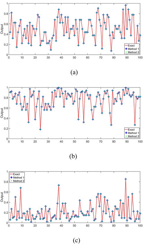
ii

be implemented using chemical neural networks [37], [38].          implemented using molecular computing and DNA where the
DNA Hopfield neural networks [39] and DNA multi-layer              weights can be arbitrary and only the inputs must correspond
perceptrons were implemented based on the operations of            to bipolar format. The latter is not a concern as features are
vector algebra including inner and outer products in DNA           typically normalized to the dynamic range [−1, 1].
vector space by mapping the concentrations of single-stranded         This paper makes four contributions. First molecular per-
DNA to amplitudes of basis vectors [40], [41]. A DNA               ceptrons that can handle arbitrary weights and can compute
transcriptional switch was proposed to design feed-forward         sigmoid of the weighted sums are presented. Thus, these
networks and winner-take-all networks [42]. A DNA-based            molecular perceptrons are ideal for regression applications
molecular pattern classification was developed based on the        unlike prior molecular perceptrons [55]. A new molecular
competitive hybridization reaction between input molecules         divider is introduced and is used to compute sigmoid(ax)
and a differentially labeled probe mixture [43]. A multi-gene      where a > 1; this circuit overcomes the scaling bottleneck.
classification was proposed based on a series of reactions         Second, a molecular implementation of an artificial neural
that compute the inner product between RNA inputs and              network (ANN) with one hidden layer is presented. It may
engineered DNA probes [44]. In [45], Poole et al. have shown       be noted that such a molecular ANN with non-binary inputs
that a Boltzmann machine could be implemented by using a           has not been presented before. Third, a trained ANN clas-
stochastic chemical reaction network.                              sifier with one hidden layer from seizure prediction using
   Arbitrary linear threshold circuits could be systematically     electroencephalogram [56] is mapped to molecular reactions
transformed into DNA strand displacement cascades [46], [47].      and DNA. The Software package from David Soloveichik et
This implementation allows designers to build complex arti-        al. is used to simulate the Chemical Reaction Networks and
ficial neural networks like Hopfield associative memory [46].      their corresponding DNA implementations presented in this
Winner-take-all neural networks with binary inputs have been       paper [13].
implemented using DSD reactions in [47]. These molecular              Although the sigmoid activation function is used for the hid-
and DNA ANNs hold the promise for processing the protein           den layer in the application considered in this paper, rectified
concentrations as features and output a decision variable          linear unit (ReLU) and softmax activation functions are used
that can be used to take an action such as monitoring a            in many neural networks. Molecular and DNA reactions for
protein or delivering a drug [48]–[52]. With a variable-gain       implementing ReLU and softmax functions are also presented
amplifier [53], [54], these DNA ANNs could also be used to         in this paper. We believe molecular ReLU and molecular
process non-DNA inputs such as RNA or protein [47].                softmax units have not been presented before.
   The DNA neural network in Cherry and Qian [47] assumes             This paper is organized as follows. Section II briefly
all inputs to be binary and weights to be non-negative.            introduces fractional coding. Simple molecular gates using
Furthermore, in Qian, Winfree and Bruck [46], weights can          fractional coding are also reviewed in Section II. Section III
be arbitrary; however, inputs are still assumed to be binary.      addresses the approaches for mapping specific target functions
The linear classifier with two arbitrary inputs but one positive   to molecular reactions. Mapping of molecular reactions to
weight and one negative weight was proposed in Zhang               DNA is described in Section IV. Molecular reactions for im-
and Seelig [53]. Furthermore, in Chen and Seelig [54], the         plementing a single-layer neural network regression (also re-
two weights of a linear classifier can be arbitrary; however       ferred to as a perceptron) and corresponding simulation results
the summation part of linear classifier is not computed by         with three different sets of weights are described in Section V.
CRNs [54]. In the current paper, the inputs are bounded            Section VI discusses the molecular and DNA implementations
between -1 and 1, and the weights can be arbitrary and not         of ANN classifier and presents experimental results of the
necessarily bounded to [−1, 1].                                    proposed architectures based on an ANN trained for seizure
   Using fractional coding, molecular gates for multiplication,    prediction from electroencephalogram (EEG) signals. Section
addition, inner product, and the perceptron function were pre-     VII presents molecular and DNA implementations of ReLU
sented in [55]. However, thePperceptron presented in [55] can      and softmax activation functions. Finally, some conclusions
                               N
only compute sigmoid( N1 i=1 wi xi ) and cannot compute            are given in Section VIII.
           PN
sigmoid( i=1 wi xi ). These perceptrons compute sigmoid of
the scaled weighted sum of the inputs; these cannot compute
                                                                     II. M OLECULAR G ATES USING F RACTIONAL C ODING
sigmoid of the weighted sum without scaling. Therefore, these
perceptrons are only useful in classification but not regression      Fractional coding was introduced in [29], [57] and was
applications. Furthermore, wi and xi must be representable in      used to realize Markov chains and polynomial computations
bipolar format in fractional coding. In many machine learning      using molecular reactions and DNA. Fractional coding is
problems, the weights can be greater than 1 in magnitude.          inspired by stochastic logic in electronic computing [58]–[77].
These weights cannot be handled by the approach in [55].           More recently, stochastic logic was shown to be equivalent
Thus, two major limitations of the approach in [55] include        to molecular computing based on fractional coding [55]. In
inability to handle arbitrary weights and inability to compute     fractional coding, each value is encoded using two molecules.
exact sigmoid function of the weighted sum of the inputs.          For example, value X can be encoded as X1 /(X1 + X0 ) where
Whether molecular perceptrons that can implement sigmoid           X1 and X0 , respectively, represent the molecules of type-1 and
of weighted inputs are synthesizable has remained an open          type-0. In stochastic logic, X1 and X0 , respectively, represent
question. This paper shows that such perceptrons can indeed be     the number of 1 and 0 bits in a unary bit stream [58]. Due to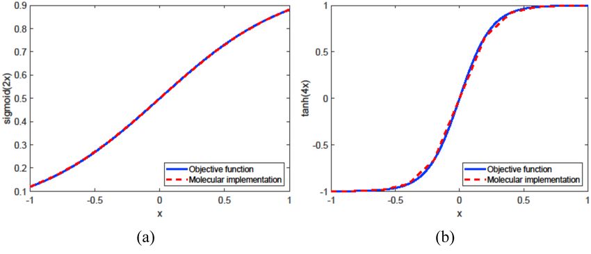
iii
the equivalence, any known stochastic logic system forms the compute sigmoid, tangent hyperbolic functions and percep-
basis for a molecular computing system. It was pointed out in trons. This section reviews implementation of exponential
[55] that stochastic digital filters and stochastic error control functions as described by Parhi and Liu [78]. Stochastic logic
coders such as low-density parity check [64] and polar code architectures presented in [61], [77] contain feedback and
decoders [65], [66] can be easily mapped to molecular digital are not easily adaptable to molecular computing. The tangent
filters and molecular error control coders. hyperbolic and sigmoid functions are inspired by the stochastic
In stochastic logic, the numbers can be represented in either logic implementation proposed by Liu and Parhi [74]. The
unipolar or bipolar format. In the unipolar format, the value of stochastic logic implementation of the sigmoid function in [79]
a variable is determined by the fraction of the concentrations does not require explicit computation of the sigmoid function
of two assigned molecular types: as it makes use of hybrid representation [75]; however, it
cannot compute sigmoid(ax) where a > 1 as required for
[X1 ] the regression function presented in this paper.
x=
[X0 ] + [X1 ]
A. Implementation of Exponential Functions in Unipolar For-
where [X0 ] and [X1 ] represent the concentrations of the
mat
assigned molecular types X0 and X1 , respectively. Note that
the numbers in the unipolar representation must lie in the unit The function e−ax (0 < a ≤ 1) can be approximated as:
interval, [0, 1]. In the bipolar format, a number x in the range
[−1, 1] can be represented using molecular types X1 and X0 a2 x2 a3 x3 a4 x4 a5 x5
such that: e−ax ≈ 1 − ax + − + −
2! 3! 4! 5!
ax ax ax ax
= 1 − ax(1 − (1 − (1 − (1 − )))) (1)
[X1 ] − [X0 ] 2 3 4 5
x=
[X0 ] + [X1 ] where e−ax is approximated by a 5th -order truncated
Maclaurin series and then reformulated by Horner’s rule. In
where [X0 ] and [X1 ] represent the concentrations of the
equation (1), all coefficients, a, a2 , a3 , a4 and a5 , can be repre-
molecular types X0 and X1 , respectively.
sented using unipolar format while 0 < a ≤ 1. Fig. 3 shows
x x x x x the stochastic implementation of e−ax by cascading AND and
z z z z z
y y y y NAND gates. The unipolar Mult and unipolar NMult units
y
s discussed before compute the same operations as AND and
X 0 + Y0 → Z 0 X 0 + Y0 → Z1 X 0 + Y0 → Z1 X 0 + Y0 → Z 0 X 0 + S0 → Z 0 NAND in stochastic implementation, respectively. So equation
X 0 + Y1 → Z 0 X 0 + Y1 → Z1 X 0 + Y1 → Z 0 X 0 + Y1 → Z1 X 1 + S0 → Z1
X 1 + Y0 → Z 0 X 1 + Y0 → Z1 X 1 + Y0 → Z 0 X 1 + Y0 → Z1 Y0 + S1 → Z 0
(1) can be implemented using unipolar Mult and unipolar
X 1 + Y1 → Z1 X 1 + Y1 → Z 0 X 1 + Y1 → Z1 X 1 + Y1 → Z 0 Y1 + S1 → Z1 NMult units shown in Figs. 2 (a) and (b), respectively [55].
z = x y z = 1− x y z = x y z =−x y z = (1−s) x + s y
(a) (b) (c) (d) (e)
x
Fig. 2: Basic molecular units. (a) Unipolar Mult unit. (b) a/5
a/4 a/3 a/2
Unipolar NMult unit. (c) Bipolar Mult unit. (d) Bipolar
NMult unit. (e) Unipolar/Bipolar MUX unit. This is taken from Fig. 3: Stochastic implementation of e−ax using 5th -order
[55]. Maclaurin expansion and Horner’s rule [78].
Molecular reactions for five basic units have been presented With a > 1, the coefficients in equation (1) may be
in [55] and are shown in Fig. 2. Fig. 2(a) shows four molecular larger than 1 which cannot be represented using fractional
reactions of the unipolar Mult unit that compute the unipolar representation. Therefore, e−ax (a > 1) cannot be directly
product of two unipolar inputs, z = x×y. The unipolar NMult implemented using this method. However, e−ax (a > 1) can
unit, consisting of four molecular reactions, shown in Fig. 2(b), be implemented by cascading the output of e−bx (b ≤ 1) [78].
computes z = 1 − x × y where x and y are the unipolar inputs For example, the function e−3x can be expressed as:
and z is the unipolar output. Bipolar Mult and NMult units
shown in Figs. 2(c) and (d) compute z = x×y and z = −x×y,
respectively, where x and y are the bipolar inputs and z is the e−3x = e−x · e−x · e−x .
bipolar output. Unipolar and bipolar MUX units that compute Fig. 4 shows the stochastic implementation of e−3x based
z = (1 − s) × x + s × y can be implemented by using the on the stochastic circuit of e−x shown in Fig. 3.
four molecular reactions shown in Fig. 2(e). For unipolar MUX
unit, x, y, z and s are all in unipolar format. But for bipolar e x
e 3x
MUX unit, x, y and z are in bipolar format whereas s is in
unipolar format.
III. M OLECULAR R EACTIONS FOR C OMPUTING Fig. 4: Stochastic implementation of e−3x using e−x and two
F UNCTIONS cascaded AND gates.
This section reviews molecular implementation of expo- For any arbitrary a which is greater than 1, e−ax can be
nential functions, and then presents molecular reactions to described by: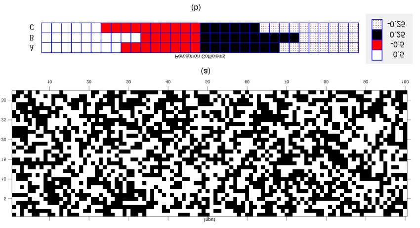
iv

                           N                                                         d[X0 ]
                           Y                  a                                                       = −[X0 ][Y0 ] − [X0 ][Y1 ]
                  e−ax =         e−bx , b =     .                                      dt
                           n=1
                                              N                                      d[X1 ]
                                                                                                      = −[X1 ][Y0 ] − [X1 ][Y1 ]
                                                                                       dt
                                                                                     d[Y0 ]
   where 0 < b ≤ 1 and N is an integer. Notice that, for b ≤ 1,                                       = −[X0 ][Y0 ] − [X1 ][Y0 ]
e−bx can always be implemented using the circuit shown in                              dt
                                                                                     d[Y1 ]
Fig. 3. Fig. 5 shows the implementation of e−ax based on e−bx                                         = −[X0 ][Y1 ] − [X1 ][Y1 ]
and N − 1 cascaded AND gates as presented in [78]. Due to                              dt
                                                                                     d[Z0 ]
the equivalence of AND in stochastic logic and unipolar Mult                                          =   [X0 ][Y1 ] + [X1 ][Y1 ]
unit shown in Fig. 2(a), N − 1 cascaded unipolar Mult units                            dt
                                                                                     d[Z1 ]
perform the same computation as N − 1 cascaded AND gates.                                             =   [X1 ][Y0 ] + [X1 ][Y1 ].             (2)
Therefore, e−ax with large a can be implemented by using                               dt
unipolar Mult and NMult units as shown in Fig. 5. The                 Using the ODE equations in (2) we can prove that the CRN
Mult and NMult units can be mapped to their equivalent             for DIV unit computes the division in fractional coding. The
molecular reactions as shown in Fig. 2, respectively.              first four equations of (2) can be rewritten as:

                                                                                      d[X0 ]
                                                                                                       = −([Y0 ] + [Y1 ])dt
                                                                                       X0
                                                                                      d[X1 ]
                                                                                                       = −([Y0 ] + [Y1 ])dt
Fig. 5: Stochastic implementation of e−ax by cascading e−x                             X1
and a − 1 AND gates.                                                                  d[Y0 ]
                                                                                                       = −([X0 ] + [X1 ])dt
                                                                                        Y0
                                                                                      d[Y1 ]
                                                                                                       = −([X0 ] + [X1 ])dt.                   (3)
                                                                                        Y1
B. Implementation of Division Functions in Unipolar Format           Comparing the first two equations of (3) we have

                                                                        Z    t              Z     t               Z   t
                                                                                 d[X0 ]               d[X1 ]
                                                                                        =                    =            −([Y0 ] + [Y1 ])dt
                                                                         0        [X0 ]       0       [X1 ]       0
                                                                                                                                               (4)

                                                                     Suppose x0 and x1 represent the initial concentrations for
                                                                   the molecules X0 and X1 , respectively. From (4) we have

                                                                                      ln[X0 ] − ln x0 = ln[X1 ] − ln x1
                                                                                                          [X0 ]       [X1 ]
                                                                                                      ⇒    x0     =    x1 .                    (5)

                                                                     Similarly, from the last two reactions in (3) we obtain

                                                                                                      [Y0 ]   [Y1 ]
                                                      x
Fig. 6: The division unit. This unit calculates z = x+y  , the                                              =                                  (6)
                                                                                                       y0      y1
division of two input variables x and y in unipolar fractional
representation.                                                    where y0 and y1 are the initial concentrations for the molecules
                                                                   Y0 and Y1 , respectively. The initial values for molecules Z0
   Implementation of molecular dividers has not been pre-          and Z1 are zero and we can write
sented before. This section presents a new molecular divider
using fractional coding; this design is not inspired by stochas-                         [Z1 ]
                                                                                                                  d[Z1 ]
                                                                                                                    dt
tic logic dividers. The four molecular reactions shown in                                          =         d[Z0 ]    d[Z1 ]
                                                                                                                                 .             (7)
                                                                                     [Z0 ] + [Z1 ]                  +
Fig. 6 compute z as the division of x and x + y using two                                                      dt        dt
                                                         [X1]
inputs x and y, all in unipolar format. So if x = [X0]+[X1]
             [Y 1]                  [Z1]        x
                                                                     From the last two equations of (2) we write
and y = [Y 0]+[Y   1] then z = [Z0]+[Z1] = x+y . For these
reactions shown in Fig. 6, the mass kinetics are described by              [Z1 ]              [X1 ][Y0 ] + [X1 ][Y1 ]
the ordinary differential equations (ODEs):                                          =                                       .                 (8)
                                                                       [Z0 ] + [Z1 ]   [X0 ][Y1 ] + 2[X1 ][Y1 ] + [X1 ][Y0 ]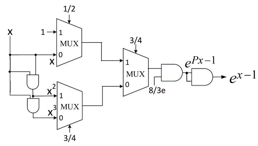
v
By substituting (5) and (6) into (8) we obtain
1 − e−2ax
[Z1 ] tanh(ax) =
z = 1 + e−2ax
[Z0 ] + [Z1 ] 1
y0 = 2· −1
y1 [X1 ][Y1 ] + [X1 ][Y1 ] 1 + e−2ax
= x0 y0
x1 [X1 ][Y1 ] + 2[X1 ][Y1 ] + y1 [X1 ][Y1 ]
= 2 · sigmoid(2ax) − 1.
y0
y1 + 1 Given −1 ≤ x ≤ 1, sigmoid(2ax) is in the range
= x0 y0
x1 + 2 + y1
[0, 1] represented in unipolar format. So if sigmoid(2ax) =
[S1 ] [S1 ] [S1 ]−[S0 ]
x1 (y0 + y1 ) [S0 ]+[S1 ] , then tanh(ax) = 2 · [S0 ]+[S1 ] − 1 = [S0 ]+[S1 ] .
= Recall the definition of bipolar format x = [X 1 ]−[X0 ]
x1 (y0 + y1 ) + y1 (x0 + x1 ) [X0 ]+[X1 ] , where
x1
x [X0 ] and [X1 ] represent the corresponding concentrations of
x0 +x1
= x1 y1 = . (9) the assigned molecular types while x represents the bipolar
x1 +x0 + y1 +y0 x + y
value. We can observe that both functions can be implemented
using the same molecular circuit shown in Fig. 7, where
the output concentrations in unipolar representation compute
C. Implementations of Sigmoid Functions and Tangent Hyper- sigmoid(2ax) whereas the output in bipolar representation
bolic in Bipolar Format computes tanh(ax). Molecular sigmoids and molecular tan-
Implementation of sigmoid functions requires computing gent hyperbolic functions have not been presented before.
sigmoid(ax) where a can be greater than 1. This computation These are typically used as activation functions of perceptrons
is reformulated using a division operation. The divider of the and ANNs.
previous subsection is used in this subsection. Fig. 8 shows the simulation results of sigmoid(2x) and
tanh(4x) using the proposed approach shown in Fig. 7 with
Consider the implementation of sigmoid(2ax) (a > 0) with
5th -order truncated Maclaurin expansion of e−x . We show
bioplar input and unipolar output as follows [74]:
CRNs of sigmoid(2x) in Supplementary Section S.3.
1
sigmoid(2ax) = (10)
1 + e−2ax
1
= −2a(2P
(11)
1+e x −1)
1
= (12)
1 + e−4aPx · e2a
e−2a
= −2a
. (13)
e + e−4aPx
In equation (11), x is replaced by 2Px − 1 where Px Fig. 8: Simulation results of bipolar (a) sigmoid(2x) and (b)
represents the unipolar value of the input bit stream while the tanh(4x) implemented by using molecular reactions shown in
output is also in unipolar format. So sigmoid(2ax) can be Figs. 2 and 6 with the proposed design shown in Fig. 7.
implemented in unipolar logic. The molecular implementation
is shown in Fig. 7. In this design, e−2a (a > 0) is in the
D. Computing Scaled Inner Products
range of [0,1] which can be represented in unipolar format by PN
using a pair of molecular types. The e−4aPx is implemented Notice that inner product ( i=1 wi xi ) cannot be directly
using the proposed method in Section III.A based on molecular implemented since the result might not be bounded by −1 and
reactions. Then sigmoid(2ax) can be implemented by using 1, which violates the constraint of bipolar format. Therefore,
the division function presented in Section III.B with two inputs scaled versions of inner product are needed. In this section,
e−2a and e−4aPx . two molecular approaches to computing scaled inner product
of two inputs vectors in bipolar format are presented.
1) Inner Number of Inputs: Given
Products Scaled by the
DIV
e −2a
x1 w1
sigmoid(2ax) in unipolar x2 w2
x = : and w = : as the two input vectors
tanh(ax) in bipolar
e −4 aPx xN wN
where each element is in bipolar format, we can compute
the inner product functions scaled by the number of inputs
Fig. 7: Stochastic implementation of sigmoid(2ax) and N with 4N molecular reactions as shown in Fig. 9 [55].
tanh(ax) with positive a. Each of the four reactions is related to a bipolar Mult unit
shown in Fig. 2(c) with two corresponding inputs, xi and
Consider tanh(ax) with positive a described as follows: wi . Fig. 9 also lists the proposed molecular reactions, where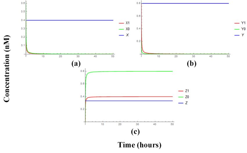
vi
i = 1, 2, · · · N . Notice that −1 ≤ xi ≤ 1, −1 ≤ wi ≤ 1
must be guaranteed for feasible design. So if xi = [Xi 1 ]−[Xi0 ]
[Xi1 ]+[Xi0 ]
PN
and wi = [W i1 ]−[W i0 ] [Y1 ]−[Y0 ] 1
[W i1 ]+[W i0 ] then y = [Y1 ]+[Y0 ] = N i=1 wi xi .
A proof of the functionality of the molecular inner product
in Fig. 9 is described in Section S.5 of the Supplementary
Information in [55].
x
y
w
Xi0 + Wi0 → Y1
Xi0 + Wi1 → Y0 1 N Fig. 10: The inner product unit II (a) with 2-dimensional
y= wx input vectors that calculates y = |w1 |+|w1
(w1 x1 + w2 x2 )
Xi1 + Wi0 → Y0 N i =1 i i 2|
Xi1 + Wi1 → Y1 and (b) with P N -dimensional input vectors that calculates
N
z = PN 1 |w | ( i=1 wi xi ) based on two N2 -dimensional inner
i=1 i
Fig.P9: The inner product unit I. This unit calculates y = products. In both cases, each element xi is in bipolar fractional
1 N
N i=1 wi xi , the scaled inner product of two input vectors representation and each element wi takes arbitrary values..
x and w where each element is in bipolar fractional represen-
tation.
N
2) Inner Products Scaled by the Sum of Absolute Value 2
[Y11 ] − [Y10 ] 1 X
of Weights: In most ANNs, trained weights need not be y1 = = PN w i xi
guaranteed to lie between −1 and 1 when the result of the inner [Y11 ] + [Y10 ] 2
|w | i=1
i=1 i
product function scaled by the number of inputs as shown in [Y21 ] − [Y20 ] 1 XN
Fig. 9 might be out of range for bipolar representation. The y2 = = PN wi xi
[Y21 ] + [Y20 ] i= N +1 |wi | i= N +1
stochastic implementation of inner product scaled by sum of 2 2
the absolute weights was proposed in [68], [80]. This method P N2
[SN 1 ] |wi |
has no limitation on the range of elements in one input vector sN = = Pi=1
N
while the elements in the other input vector must be in range [SN 1 ] + [SN 0 ] i=1 |wi |
[−1, 1]. Consider the basic condition
when the dimension of [Z1 ] − [Z0 ]
x1
z = = sN · y1 + (1 − sN ) · y2 . (14)
the input vectors is 2, where x = (−1 ≤ xi ≤ 1) and [Z1 ] + [Z0 ]
x2
w1 Notice that equation (14) computes the scaled inner product
w= (wi ∈ R). In this approach, the MUX units are used (z) of two N -dimensional input vectors, x and w, by using a
w2
to perform addition and the Mult units are used to perform MUX unit with the inputs y1 and y2 of two inner-product func-
multiplication as shown in Fig. 10. Select signal of multiplexer tions with corresponding halves of the input vectors while the
PN
is given by: s2 = |w1|w 1|
|+|w2 | . select signal of the multiplexer is given by: sN = PNi=1
2
i
.
|w |
i=1 |wi |
Fig. 10(a) describes a two-input inner product where x1 Fig. 10 shows the corresponding circuit diagram P
and molecular
and x2 are in bipolar format and the pre-calculated coefficient N
reactions for the implementation of PN 1 |w | i=1 wi xi in
s2 is in unipolar format. Fig. 10(a) also lists the proposed i=1 i
bipolar format using equation (14). Inner product functions
molecular reactions. Besides, a1 and a2 represent signs of w1 with odd-dimensional input vectors can also be implemented
and w2 , respectively. If wi > 0, then ai = [a i1 ]−[ai0 ]
[ai1 ]+[ai0 ] = 1. using the approach shown in Fig. 10(b) by adding an extra
[ai1 ]−[ai0 ] [X11 ]−[X1 0 ]
Otherwise, ai = [ai1 ]+[ai0 ] = −1. So given X1 = [X11 ]+[X10 ] , input feature with zero weight.
X2 = [X 21 ]−[X20 ] [S2 1 ]
[X21 ]+[X2 0 ] and S2 = [S21 ]+[S20 ] , then final output is
given by: y = [Y 1 ]−[Y0 ] 1
[Y1 ]+[Y0 ] = |w1 |+|w2 | (w1 x1 + w2 x2 ). Note that
IV. M APPING M OLECULAR C OMPUTING S YSTEM TO DNA
a 4-input inner product can be computed recursively using two Abstract chemical reaction networks (CRNs) described by
2-input inner products at first-level and then another 2-input molecular reactions can be mapped to DNA strand displace-
inner product at second-level. The recursive formulation leads ment (DSD) reactions as shown in [55]. The DSD reactions
to a tree-based design [68]. based on toehold mediation was primarily introduced by Yurke
An inner product with N -dimensional input vectors can be et al. in [15]. A framework that can implement arbitrary
implemented based on two inner products with N2 -dimensional molecular reactions with no more than two reactants by lin-
input vectors as shown in Fig. 10(b).
PNConsider the stochastic ear, double-stranded DNA complexes was proposed by Chen
implementation of z = PN 1 |w | i=1 wi xi , which can be in [81]. Notice that our computational units are all built based
i=1 i
written as follows: on molecular reactions with at most two reactants. We simulatevii
the ANN classifier for the EEG signal classification by using C. Each weight, 1/2, −1/2, 1/4 and −1/4, occurs 8 times
the software package provided by Winfree’s team at Caltech in Perceptron A. The same weights occur 10, 6, 10 and 6
[13]. More details of mapping bimolecular reactions to DSD times, respectively, in Perceptron B; and 6, 10, 6 and 10 times,
are described in Section S.8 of the Supplementary Information respectively, in Perceptron C.
of [55].
V. M OLECULAR AND DNA P ERCEPTRONS WITH B INARY
I NPUTS AND N ON -B INARY W EIGHTS
In this section, we present the implementation of a single-
layer neural network, also called a perceptron, using molecular
reactions. The perceptronP is illustrated in Fig. 11(a) where
N
the weighted sum y = i=1 wi xi is computed first. The
final output z is then computed as z = sigmoid(y). The
molecular inner products cannot compute the inner product
exactly, but can compute only a scaled version of the inner
product. Figs. 11(b) and (c) illustrate two approaches to
implement a molecular perceptron. In Fig. 11(a), the inner
product is scaled down by the number of inputs, N . In Fig. 12: Inputs, weights of three perceptrons, denoted A, B,
Fig. 11(c), the inner product is scaled C. (a) Inputs to the perceptron: each column represents an
PN down by the sum of
the absolute values of the weights i=1 |wi |. The molecular input vector containing 32 binary inputs in this 32×100 block
sigmoid, therefore, must compute the sigmoid of the scaled- matrix. Each black block corresponds to a 0 and each white
up version of the input using the molecular sigmoid(2ax) block represents a 1. (b) Weights: the weights for the three
presented in Section III. The molecular perceptrons shown perceptrons are illustrated. Each row represents the 32 weights
in Figs. 11(b) and (c) perform the same computation as the for one perceptron. These weights are divided into 4 parts and
standard perceptron shown in Fig. 11(a). The implementation correspond to 1/2, −1/2, 1/4, −1/4 from left to right. The
of computing sigmoid of the weighted sum scaled by the figure is taken from [55].
number of inputs was presented in [55]; such a sigmoid cannot
be used for regression applications. The proposed molecular Three perceptrons are simulated by using the two methods
perceptrons in Figs. 11(b) and (c) compute the exact sigmoid shown in Figs. 11(b) and (c). The first method cascades
and can be used for regression applications. the inner product units scaled by the number of inputs and
sigmoid(32x) which can be implemented by setting a = 16 in
sigmoid y sigmoid Ny
x1 x1
w1 w1 the approach illustrated in Fig. 7. The second method cascades
x2 w2 x2 w2
the inner product units scaled by the sum of absolute weights,
y y
z z
wN wN 12; sigmoid(12x) can be implemented by setting a = 6
xN
y N wi xi xN
y 1 N wi xi in the approach illustrated in Fig. 7. Note that an approach
i 1 N i 1
to compute sigmoid(x) with implicit format conversion was
(a) (b) presented in [79]; however, this approach is not applicable
N
sigmoid w y here as we need to compute sigmoid(ax) with a greater
x1 i
w1
i 1 than 1 and not sigmoid(x). Various activation functions are
x2 w2
used in neural networks, we show how Rectified Linear Unit
y
z
wN and softmax function can be synthesized using molecular
xN y N 1 N
wi xi computing via fractional coding in Section VII.
i 1
|wi |
i 1 The molecular simulation results of the three perceptrons
(c)
are shown in Figs. 13(a)-(c), respectively. The bimolecular
Fig. 11: Molecular perceptron. (a) A standard perceptron reactions are mapped to DNA as described in [13]. The
PN
that computes sigmoid( i=1 wi xi ), (b) the molecular per- DNA simulation results of the three perceptrons are shown in
PN Figs. 14(a)-(c), respectively. The red line illustrates the target
ceptron that computes sigmoid(N · ( N1 i=1 wi xi )) and (c)
PN outputs of 100 input vectors; the blue crosses show the outputs
the molecular perceptron that computes sigmoid( i=1 |wi | ·
N of the perceptron as shown in Fig. 11(b) where the scaling
( PN 1 |w | i=1 wi xi )).
P
i=1 i of the inner product is the number of the inputs (referred
Three perceptrons are simulated with N = 32 using the 32 to as Method-1) and the green diamonds show the outputs
coefficients as described in [55]. Notice that there are 100 sets of the perceptron as shown in Fig. 11(c) where the scaling
of inputs and each set consists of 32 randomly selected binary of the inner product is the sum of the absolute value of the
numbers as shown in Fig. 12(a). However, the inputs of the coefficients (referred to as Method-2). The horizontal axis in
proposed molecular perceptron don’t have to be binary, but Fig. 13 represents the index of the input vector and the vertical
should be no less than −1 and no greater than 1. Fig. 12(b) axis shows the exact and molecular sigmoid values. The mean
shows the weights for the 3 perceptrons, denoted A, B and square error, MSE, is defined as:viii
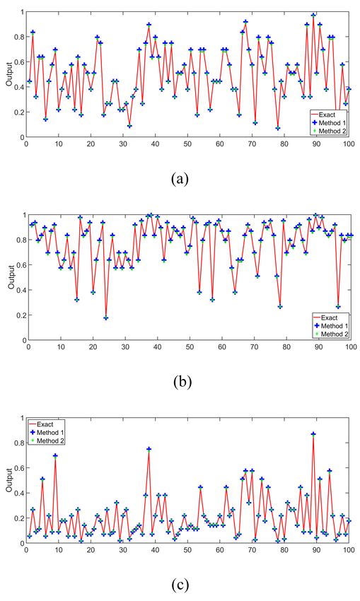
Fig. 14: Exact and molecular outputs of three perceptrons: (a)
Fig. 13: Exact and molecular outputs of three perceptrons: (a) Perceptron A, (b) Perceptron B, (c) Perceptron C. The x axis
Perceptron A, (b) Perceptron B, (c) Perceptron C. The x axis represents 100 random input vectors.
represents 100 random input vectors.
as an activation function for neurons in the hidden layer of an
ANN. These neurons need to compute exact sigmoid values.
100 Our paper describes a molecular ANN with one hidden layer
1 X 2 for a seizure prediction application. The activation functions
M SE = |z(j) − zb(j)|
100 j=1 of the hidden layer neurons do require computing sigmoid(x)
PN without scaling of inputs, and thus act as regressors. The
where z(j) = sigmoid( i=1 wi xi [j]) represents the exact outputs of these regressors are fed to the output neuron. Thus,
value, zb(j) represents the simulation result, xi [j] represents the contribution of this paper is significant in the context of
the ith bit position of input vector j, and wi is the ith weight. molecular ANNs.
The mean square error values for the molecular and DNA
simulations are listed in Table I. The proposed Method-2 A. Architecture of the Molecular Implementation
achieves less error than the Method-1. Consider the ANN with one hidden layer as shown in
Fig. 15(a). Each neuron computes a weighted sum of the neu-
VI. M OLECULAR AND DNA I MPLEMENTATION OF ANN ron values from the previous layer followed by an activation
C LASSIFIERS function (Θ). Thus, each neuron contains an inner-product and
Classification using a simple perceptron may be possible us- a tangent hyperbolic function PNas shown in Fig. 15(b). The
1
ing a sigmoid(x) function with scaled inputs. Thus, the prior inner-product PN |w
i |+|b| i=1 (wi xi + b) is computed at
i=1
work [55] may suffice to act as a classifier for a perceptron. node y by using the approach of inner product unit II as shown
However, such a sigmoid function as in [55] cannot be used in Fig. 10 with N + 1 inputs.ix
TABLE I: Mean sqaure errors for the three perceptrons using molecular reactions and DNA.
Molecular DNA
Perceptron Method 1 Method 2 Method 1 Method 2
A 1.78486 × 10⁻⁷ 2.67643 × 10⁻⁸ 1.22267 × 10⁻⁴ 4.05697 × 10⁻⁶
B 1.3643 × 10⁻⁷ 2.56013 × 10⁻⁸ 1.96767 × 10⁻⁴ 7.57364 × 10⁻⁶
C 7.29132 × 10 −8 7.66375 × 10⁻⁹ 3.69588 × 10⁻⁵ 1.89104 × 10⁻⁶
represent the number of inputs data samples and the number
of features, respectively. The linear mapping is performed for
all samples as follows:
2(Xij − min(Xi ))
Xij ⇐ , for 1 ≤ i ≤ 4, 1 ≤ j ≤ 10422
max(Xi ) − min(Xi )
where max(Xi ) and min(Xi ) represent the maximum and
minimum magnitudes of the ith feature among all 10422
samples. After this linear mapping, each element in a column
of the input matrix X has mean 0 and the dynamic range
of [−1, 1]. The histogram of 41688 features from 10422 4-
dimensional feature vectors after linear mapping is shown in
Fig. 16. The threshold for the finial classification is zero.
Table III lists the weight matrices and bias vectors of the
optimized ANN model, where wI represents the connection
weight matrix of the input-hidden layer connection, wh repre-
sents the hidden layer-output connection, bh represents the bias
column vector for the hidden neurons, and bo is the bias for the
output neuron. Fig. 17 shows the molecular implementation
Fig. 15: (a) An artificial neural network (ANN) model with one of the ANN model. This circuit includes 58 Mult units, 25
hidden layer, (b) computation kernel in a neuron implemented NMult units, 25 MUX units and 5 division units. Table II states
in molecular reactions. the number of reactants and the number of reactions for the
molecular ANN. The length of molecular simulation time is 50
Notice that the molecular implementation of tangent hy- hours. Using the coefficients of the ANN and actual data from
perbolic functions tanh(ax) is illustrated in Fig. 7. The result a patient with 10422 samples, the confusion matrices for the
computed at node y is a scaled version of the original weighted ideal classification results from MATLAB using the trained
sum. However the output of the neuron implemented by ANN and the molecular classification results are shown in
molecular reactions is the same as the output of a conven- Tables IV and V, respectively. Here the ground truth is the
tional implementation while tanh(ax) is implemented using actual label of the data from the patient. The ideal MATLAB
PN
a = round( i=1 |wi | + |b|) instead of the original tanh(x). results in Table IV are the best achievable by an ANN with one
hidden layer with five neurons. To achieve better accuracy, an
ANN with more neurons in the hidden layer or more number
B. EEG Signal Classification using Molecular ANN Classifier of hidden layers should be trained.
The molecular ANN classifier is tested using an ANN with
one hidden layer containing five neurons and four neurons for TABLE II: Number of Reactants and Reactions for Molecular
the input layer trained for an application for seizure prediction and ANN DNA Implementations.
from electroencephalogram (EEG) signals [82]. The data from
Molecular ANN DNA ANN
one human patient from the UPenn/Mayo Seizure Prediction Reactants 456 5184
Contest sponsored by the American Epilepsy Society and Reactions 678 2260
hosted by Kaggle is used for training the ANN [83]. In
prior work, the same data was used to design an ANN
using stochastic logic [56]. The testing data contains 10422
TABLE IV: The confusion matrix of classification using
samples and each sample contains a vector with 4 features
MATLAB.
(x = x1 , x2 , x3 , x4 ) and a bias term, b. Since the range of
the input features should be [−1, 1] under the constraint of Predicted
Positive Negative
bipolar format representation, a linear mapping is performed Actual Positive TP=5267 FN=124 TPR=0.9770
on the input features. Consider the input data as a 10422 × 4 Class Negative FP=368 TN=4663 TNR=0.9269
matrix X, where the number of rows (10422) and columns (4) ACC=0.9528 PPV=0.9347 NPV=0.9741x
TABLE III: Weights and bias of the optimized ANN model.
Input - Hidden layer connections Hidden layer - Output connections
Weights Bias Weights Bias
I
wj1 I
wj2 I
wj3 I
wj4 bhj wjh bo
-5.3992 -0.7689 70.3151 18.7028 20.4864 0.9229
-20.9651 -14.3900 12.9155 8.3618 0.3783 0.2838
-21.8076 -0.1503 3.8999 -4.4874 8.5850 0.6457 -0.8103
4.6043 -5.2727 -2.9103 6.3443 -0.7884 0.7392
-0.3636 -9.2811 0.5925 -0.5254 4.6805 -0.8128
TABLE VIII: The confusion matrix of classification using
DSD reactions based on molecular classification results.
Predicted
Positive Negative
Actual Positive TP=5590 FN=17 TPR=0.9970
Class Negative FP=22 TN=4793 TNR=0.9954
ACC=0.9963 PPV=0.9961 NPV=0.9965
Confusion matrices as shown in Tables VII and VIII present
the classification results from DNA classifiers based on actual
classification results and the molecular classification results
from Section IV, respectively. We can see that the ACC of
the proposed ANN using DSD reactions is 0.9517, which is
only 0.11% less than the ACC of the molecular classification.
Fig. 16: The histogram of input features after linear mapping. Table II also states the number of reactants and the number
of reactions for the DNA ANN.
TABLE V: The confusion matrix of classification using molec-
ular ANN. VII. M OLECULAR AND DNA I MPLEMENTATIONS OF
R E LU AND S OFTMAX F UNCTIONS
Predicted
Positive Negative This section describes molecular and DNA reactions for
Actual Positive TP=5250 FN=141 TPR=0.9738 implementing ReLU and softmax functions for artificial neural
Class Negative FP=357 TN=4674 TNR=0.9290
ACC=0.9522 PPV=0.9363 NPV=0.9707 networks. Molecular implementation of a Gaussian kernel has
been described in [84] in the context of a support vector
Comparing the accuracy results in Table IV with that in machine classifier.
Table V, we can find that the accuracy (ACC) of the proposed
molecular ANN is 0.9522, which is 0.06% less than the ACC A. DNA Implementation for Rectified Linear Unit
of the ideal results. Table VI shows the confusion matrix of In the context of an artificial neural network, the ReLU
molecular classification results using the ANN model where activation function is defined as:
the classification results from MATLAB represent the ground
f (x) = x+ = max(0, x) (15)
truth. It can be observed that the performance of molecular
ANN using linear mapping for input data is close to the ideal where x is the input to a neuron. Based on fractional coding,
results from MATLAB. we propose a simple set of CRNs for implementing ReLU with
inputs x ∈ [−1, 1]. Notice that ReLU activation is not needed
TABLE VI: The confusion matrix of classification using
for unipolar inputs where the output is always the same as
molecular ANN based on ideal classification results.
input. The molecular ReLU is described in Fig. 18. We show
Predicted some examples of ReLU in Supplementary Section S.2.1.
Positive Negative
Matlab Positive TP=5605 FN=30 TPR=0.9947 Fig. 19 shows the exact and simulated values of the rectified
Class Negative FP=2 TN=4785 TNR=0.9996 linear unit with bipolar inputs and bipolar outputs where the
ACC=0.9969 PPV=0.9996 NPV=0.993769 blue line represents the exact value, red circles represent the
simulated values using CRNs, and black stars represent the
C. Architecture of the DNA Implementation simulated values using DNA.
TABLE VII: The confusion matrix of classification using DSD B. DNA Implementation for Softmax function
reactions. Consider a standard softmax function with 3 different
Predicted classes with inputs yj for j = 1, 2, 3. This function is defined
Positive Negative by:
Actual Positive TP=5250 FN=141 TPR=0.9738
Class Negative FP=362 TN=4669 TNR=0.9280 eyi
ACC=0.9517 PPV=0.9355 NPV=0.9707
σ(yi ) = P3 .
yj
j=1 exi
Fig. 17: Molecular implementation of the ANN model.
Fig. 18: Molecular rectified linear unit with input x ∈ (−1, 1]. Fig. 19: Exact and computed values of the rectified linear unit.
All the reactions have the same rate. Blue lines: exact values, red circles: computed values using
CRNs, black stars: computed values using DNA.
The above can be reformulated by scaling the numerator and
denominator by e−1 . The reformulates softmax is given by: [Zj 1 ]
where zj = eyj −1 = [Zj 1 ]+[Zj 0 ] for j = 1, 2, 3.
yi
e ·e −1 The stochastic implementation of e(x−1) with unipolar input
σ(yi ) = P3 and unipolar output has been described in Parhi [76] based on
j=1 (e
yj · e−1 )
yi −1
polynomial expansion described below.
e
= P3
j=1eyj −1
zi 2 1 x 2 3 1
= . (16) e(x−1) ≈ ( + ) + ( x2 + x3 )
z1 + z2 + z3 e 2 2 3e 4 4xii
8 3 1 x 1 3 1 TABLE IX: Exact values and computed values of the softmax
= ( ( + ) + ( x2 + x3 )). (17)
3e 4 2 2 4 4 4 function with three inputs based on molecular and DNA.
Notice that the implementation of e(x−1) with bipolar input Softmax
and unipolar output can be derived based on implicit format input Exact Molecular DNA
conversion. Let x = 2Px − 1 where x is in bipolar and Px -0.2 0.195759 0.199504 0.199504
0.3 0.322752 0.326513 0.326512
is in unipolar. Then we can write: 0.7 0.481489 0.473983 0.473983
e(x−1) = e(2Px −2) (18)
(Px )−1 2
shows the exact values and computed values of the soft-
= (e ) . (19) max function with three inputs (−0.2, 0.3, 0.7) based on the
proposed molecular reactions and the corresponding DNA
implementation. The molecular implementation of the softmax
function with K different classes is shown in Supplementary
Information Section S.3.2.
VIII. C ONCLUSION
This paper has shown that artificial neural networks can be
synthesized using molecular reactions as well as DNA using
fractional coding and bimolecular reactions. While an ANN
with one hidden layer has been demonstrated, the approach
Fig. 20: Stochastic implementation of e(x−1) with bipolar applies to ANNs with multiple hidden layers. While theoretical
input. feasibility has been demonstrated by simulations, any practical
In equation (18), x is replaced by 2Px − 1 where Px use of the proposed theory still remains to be validated.
represents the unipolar value of the input bit stream while Despite lack of practical validation at this time, the theoretical
the output is also in unipolar logic. The square operation in advance is significant as it can quickly pave way for practical
equation (19) can be implemented by an AND unit with two use either in-vitro or in-vivo when the technology becomes
identical inputs (e(Px )−1 ) that is computed by using equation readily available. Future molecular sensing and computing
(17). Fig. 20 shows the implementation of e(x−1) based on systems can compute the features in-situ and these features
e(P x−1) and an AND gate. can be used for classification using molecular artificial neural
Then the softmax function with 3 inputs can be implemented networks. Future work needs to be directed towards practical
by the following molecular reactions: demonstration of the proposed theoretical framework. This
paper has addressed molecular ANNs for inference applica-
tions. Inspired by [85], a DNA perceptron that can learn was
Z10 + Z20 → I3 Z10 + Z21 → I3 presented in [86]. We caution the reader that the high accuracy
Z11 + Z20 → I3 Z11 + Z21 → I3 of the simulation of the chemical kinetics of the molecular
Z10 + Z30 → I2 Z10 + Z31 → I2 systems may not reflect the accuracy of an experiment in a
test tube for example.
Z11 + Z30 → I2 Z11 + Z31 → I2
Z20 + Z30 → I1 Z20 + Z31 → I1 R EFERENCES
Z21 + Z30 → I1 Z21 + Z31 → I1 [1] L. M. Adleman, “Molecular computation of solutions to combinatorial
Z11 + I1 → Y11 + Y20 + Y30 problems,” Science, vol. 266, no. 5187, pp. 1021–1024, 1994.
[2] M. Samoilov, A. Arkin, and J. Ross, “Signal processing by simple
Z10 + I1 → W chemical systems,” The Journal of Physical Chemistry A, vol. 106,
no. 43, pp. 10205–10221, 2002.
Z20 + I1 → W Z21 + I1 → W [3] K. Thurley, S. C. Tovey, G. Moenke, V. L. Prince, A. Meena, A. P.
Z30 + I1 → W Z31 + I1 → W Thomas, A. Skupin, C. W. Taylor, and M. Falcke, “Reliable encoding
of stimulus intensities within random sequences of intracellular ca2+
Z21 + I2 → Y10 + Y21 + Y30 spikes,” Sci. Signal., vol. 7, no. 331, pp. ra59–ra59, 2014.
[4] M. Sumit, R. Neubig, S. Takayama, and J. Linderman, “Band-pass
Z20 + I2 → W processing in a GPCR signaling pathway selects for nfat transcription
Z10 + I2 → W Z11 + I2 → W factor activation,” Integrative Biology, vol. 7, no. 11, pp. 1378–1386,
2015.
Z30 + I2 → W Z31 + I2 → W [5] Y. Park, L. Luo, K. K. Parhi, and T. Netoff, “Seizure prediction with
spectral power of EEG using cost-sensitive support vector machines,”
Z31 + I3 → Y10 + Y20 + Y31 + Z31 + I3 . Epilepsia, vol. 52, no. 10, pp. 1761–1770, 2011.
Z30 + I3 → W [6] M. Ghorbani, E. A. Jonckheere, and P. Bogdan, “Gene expression is not
random: scaling, long-range cross-dependence, and fractal characteristics
Z10 + I3 → W Z11 + I3 → W of gene regulatory networks,” Frontiers in physiology, vol. 9, p. 1446,
2018.
Z20 + I3 → W Z21 + I3 → W [7] K. K. Parhi and Z. Zhang, “Discriminative ratio of spectral power
and relative power features derived via frequency-domain model ratio
Mass-action kinetic equations for these reactions are dis- (FDMR) with application to seizure prediction,” IEEE transactions on
cussed in Supplementary Information Section S.3.1. Table IX biomedical circuits and systems, 2019.xiii
[8] H. M. Sauro and K. Kim, “Synthetic biology: it’s an analog world,” [34] E. Mjolsness, D. H. Sharp, and J. Reinitz, “A connectionist model of
Nature, vol. 497, no. 7451, p. 572, 2013. development,” Journal of Theoretical Biology, vol. 152, no. 4, pp. 429–
[9] R. Sarpeshkar, “Analog versus digital: extrapolating from electronics to 453, 1991.
neurobiology,” Neural computation, vol. 10, no. 7, pp. 1601–1638, 1998. [35] A. Hjelmfelt, E. D. Weinberger, and J. Ross, “Chemical implementation
[10] R. Daniel, J. R. Rubens, R. Sarpeshkar, and T. K. Lu, “Synthetic analog of neural networks and turing machines,” Proceedings of the National
computation in living cells,” Nature, vol. 497, no. 7451, p. 619, 2013. Academy of Sciences, vol. 88, no. 24, pp. 10983–10987, 1991.
[11] R. Sarpeshkar, “Guest editorial - special issue on synthetic biology,” [36] D. Blount, P. Banda, C. Teuscher, and D. Stefanovic, “Feedforward
IEEE transactions on biomedical circuits and systems, vol. 9, no. 4, chemical neural network: An in silico chemical system that learns xor,”
pp. 449–452, 2015. Artificial life, vol. 23, no. 3, pp. 295–317, 2017.
[12] J. J. Teo, S. S. Woo, and R. Sarpeshkar, “Synthetic biology: A unifying [37] T. Mestl, C. Lemay, and L. Glass, “Chaos in high-dimensional neural
view and review using analog circuits,” IEEE transactions on biomedical and gene networks,” Physica D: Nonlinear Phenomena, vol. 98, no. 1,
circuits and systems, vol. 9, no. 4, pp. 453–474, 2015. pp. 33–52, 1996.
[13] D. Soloveichik, G. Seelig, and E. Winfree, “DNA as a universal substrate [38] N. E. Buchler, U. Gerland, and T. Hwa, “On schemes of combinatorial
for chemical kinetics,” Proceedings of the National Academy of Sciences, transcription logic,” Proceedings of the National Academy of Sciences,
vol. 107, no. 12, pp. 5393–5398, 2010. vol. 100, no. 9, pp. 5136–5141, 2003.
[39] J. J. Hopfield, “Neural networks and physical systems with emergent
[14] D. Y. Zhang and E. Winfree, “Control of DNA strand displacement
collective computational abilities,” Proceedings of the national academy
kinetics using toehold exchange,” Journal of the American Chemical
of sciences, vol. 79, no. 8, pp. 2554–2558, 1982.
Society, vol. 131, no. 47, pp. 17303–17314, 2009.
[40] A. P. Mills Jr, B. Yurke, and P. M. Platzman, “Article for analog vector
[15] B. Yurke, A. J. Turberfield, A. P. Mills Jr, F. C. Simmel, and J. L. algebra computation,” Biosystems, vol. 52, no. 1-3, pp. 175–180, 1999.
Neumann, “A DNA-fuelled molecular machine made of DNA,” Nature, [41] A. Mills Jr, M. Turberfield, A. J. Turberfield, B. Yurke, and P. M.
vol. 406, no. 6796, p. 605, 2000. Platzman, “Experimental aspects of DNA neural network computation,”
[16] A. J. Turberfield, J. Mitchell, B. Yurke, A. P. Mills Jr, M. Blakey, and Soft Computing, vol. 5, no. 1, pp. 10–18, 2001.
F. C. Simmel, “DNA fuel for free-running nanomachines,” Physical [42] J. Kim, J. Hopfield, and E. Winfree, “Neural network computation
review letters, vol. 90, no. 11, p. 118102, 2003. by in vitro transcriptional circuits,” in Advances in neural information
[17] B. Yurke and A. P. Mills, “Using DNA to power nanostructures,” Genetic processing systems, pp. 681–688, 2005.
Programming and Evolvable Machines, vol. 4, no. 2, pp. 111–122, 2003. [43] H.-W. Lim, S. H. Lee, K.-A. Yang, J. Y. Lee, S.-I. Yoo, T. H. Park, and
[18] T. S. Gardner, C. R. Cantor, and J. J. Collins, “Construction of a genetic B.-T. Zhang, “In vitro molecular pattern classification via DNA-based
toggle switch in escherichia coli,” Nature, vol. 403, no. 6767, p. 339, weighted-sum operation,” Biosystems, vol. 100, no. 1, pp. 1–7, 2010.
2000. [44] R. Lopez, R. Wang, and G. Seelig, “A molecular multi-gene classifier
[19] R. Weiss, S. Basu, S. Hooshangi, A. Kalmbach, D. Karig, R. Mehreja, for disease diagnostics,” Nature chemistry, vol. 10, no. 7, p. 746, 2018.
and I. Netravali, “Genetic circuit building blocks for cellular compu- [45] W. Poole, A. Ortiz-Munoz, A. Behera, N. S. Jones, T. E. Ouldridge,
tation, communications, and signal processing,” Natural Computing, E. Winfree, and M. Gopalkrishnan, “Chemical boltzmann machines,”
vol. 2, no. 1, pp. 47–84, 2003. in International Conference on DNA-Based Computers, pp. 210–231,
[20] H. Jiang, M. D. Riedel, and K. K. Parhi, “Digital logic with molecular Springer, 2017.
reactions,” in Proceedings of the International Conference on Computer- [46] L. Qian, E. Winfree, and J. Bruck, “Neural network computation with
Aided Design, pp. 721–727, IEEE Press, 2013. DNA strand displacement cascades,” Nature, vol. 475, no. 7356, p. 368,
[21] H. Jiang, M. Riedel, and K. Parhi, “Synchronous sequential computation 2011.
with molecular reactions,” in Proceedings of the 48th Design Automation [47] K. M. Cherry and L. Qian, “Scaling up molecular pattern recognition
Conference, pp. 836–841, ACM, 2011. with DNA-based winner-take-all neural networks,” Nature, vol. 559,
[22] Y. Benenson, B. Gil, U. Ben-Dor, R. Adar, and E. Shapiro, “An no. 7714, p. 370, 2018.
autonomous molecular computer for logical control of gene expression,” [48] P. Mohammadi, N. Beerenwinkel, and Y. Benenson, “Automated design
Nature, vol. 429, no. 6990, p. 423, 2004. of synthetic cell classifier circuits using a two-step optimization strat-
[23] D. Endy, “Foundations for engineering biology,” Nature, vol. 438, egy,” Cell systems, vol. 4, no. 2, pp. 207–218, 2017.
no. 7067, p. 449, 2005. [49] Z. Xie, L. Wroblewska, L. Prochazka, R. Weiss, and Y. Benenson,
[24] K. I. Ramalingam, J. R. Tomshine, J. A. Maynard, and Y. N. Kaznessis, “Multi-input rnai-based logic circuit for identification of specific cancer
“Forward engineering of synthetic bio-logical and gates,” Biochemical cells,” Science, vol. 333, no. 6047, pp. 1307–1311, 2011.
Engineering Journal, vol. 47, no. 1-3, pp. 38–47, 2009. [50] Y. Li, Y. Jiang, H. Chen, W. Liao, Z. Li, R. Weiss, and Z. Xie, “Mod-
[25] A. Tamsir, J. J. Tabor, and C. A. Voigt, “Robust multicellular computing ular construction of mammalian gene circuits using tale transcriptional
using genetically encoded nor gates and chemical wires,” Nature, repressors,” Nature chemical biology, vol. 11, no. 3, p. 207, 2015.
vol. 469, no. 7329, p. 212, 2011. [51] K. Miki, K. Endo, S. Takahashi, S. Funakoshi, I. Takei, S. Katayama,
[26] H. Jiang, M. D. Riedel, and K. K. Parhi, “Digital signal processing with T. Toyoda, M. Kotaka, T. Takaki, M. Umeda, et al., “Efficient detection
molecular reactions,” IEEE Design & Test of Computers, vol. 29, no. 3, and purification of cell populations using synthetic microrna switches,”
pp. 21–31, 2012. Cell Stem Cell, vol. 16, no. 6, pp. 699–711, 2015.
[52] M. K. Sayeg, B. H. Weinberg, S. S. Cha, M. Goodloe, W. W. Wong, and
[27] H. Jiang, S. A. Salehi, M. D. Riedel, and K. K. Parhi, “Discrete-time
X. Han, “Rationally designed microrna-based genetic classifiers target
signal processing with DNA,” ACS synthetic biology, vol. 2, no. 5,
specific neurons in the brain,” ACS synthetic biology, vol. 4, no. 7,
pp. 245–254, 2013.
pp. 788–795, 2015.
[28] S. A. Salehi, H. Jiang, M. D. Riedel, and K. K. Parhi, “Molecular sensing [53] D. Y. Zhang and G. Seelig, “DNA-based fixed gain amplifiers and linear
and computing systems,” IEEE Transactions on Molecular, Biological classifier circuits,” in International Workshop on DNA-Based Computers,
and Multi-Scale Communications, vol. 1, no. 3, pp. 249–264, 2015. pp. 176–186, Springer, 2010.
[29] S. A. Salehi, M. D. Riedel, and K. K. Parhi, “Markov chain computations [54] S. X. Chen and G. Seelig, “A DNA neural network constructed from
using molecular reactions,” in 2015 IEEE international conference on molecular variable gain amplifiers,” in International Conference on
digital signal processing (DSP), pp. 689–693, IEEE, 2015. DNA-Based Computers, pp. 110–121, Springer, 2017.
[30] S. A. Salehi, M. D. Riedel, and K. K. Parhi, “Asynchronous discrete- [55] S. A. Salehi, X. Liu, M. D. Riedel, and K. K. Parhi, “Computing
time signal processing with molecular reactions,” in 2014 48th Asilomar mathematical functions using DNA via fractional coding,” Scientific
conference on signals, systems and computers, pp. 1767–1772, IEEE, reports, vol. 8, no. 1, p. 8312, 2018.
2014. [56] Y. Liu, H. Venkataraman, Z. Zhang, and K. K. Parhi, “Machine learning
[31] P. Senum and M. Riedel, “Rate-independent constructs for chemical classifiers using stochastic logic,” in 2016 IEEE 34th International
computation,” PloS one, vol. 6, no. 6, p. e21414, 2011. Conference on Computer Design (ICCD), pp. 408–411, IEEE, 2016.
[32] J. Kim, K. S. White, and E. Winfree, “Construction of an in vitro bistable [57] S. A. Salehi, K. K. Parhi, and M. D. Riedel, “Chemical reaction networks
circuit from synthetic transcriptional switches,” Molecular systems biol- for computing polynomials,” ACS synthetic biology, vol. 6, no. 1, pp. 76–
ogy, vol. 2, no. 1, p. 68, 2006. 83, 2016.
[33] A. J. Genot, J. Bath, and A. J. Turberfield, “Combinatorial displacement [58] B. R. Gaines, “Stochastic computing,” in Proceedings of the April 18-20,
of DNA strands: application to matrix multiplication and weighted 1967, spring joint computer conference, pp. 149–156, ACM, 1967.
sums,” Angewandte Chemie International Edition, vol. 52, no. 4, [59] B. R. Gaines, “Stochastic computing systems,” in Advances in informa-
pp. 1189–1192, 2013. tion systems science, pp. 37–172, Springer, 1969.You can also read