Learning Intra-Batch Connections for Deep Metric Learning
←
→
Page content transcription
If your browser does not render page correctly, please read the page content below
Learning Intra-Batch Connections for Deep Metric Learning

                                Jenny Seidenschwarz 1 Ismail Elezi 1 Laura Leal-Taixé 1

                         Abstract                                  To learn the mapping function, current approaches utilize
                                                                   siamese networks (Bromley et al., 1994), typically trained
     The goal of metric learning is to learn a function            using loss functions that measure distances between pairs
     that maps samples to a lower-dimensional space                of samples of the same class (positive) or different classes
     where similar samples lie closer than dissimilar              (negative). Contrastive loss (Bromley et al., 1994) mini-
     ones. Particularly, deep metric learning utilizes             mizes the distance of the feature embeddings for a positive
     neural networks to learn such a mapping. Most                 pair, and maximizes their distance otherwise. Triplet loss
     approaches rely on losses that only take the re-              (Schultz & Joachims, 2003; Weinberger & Saul, 2009) takes
     lations between pairs or triplets of samples into             a triplet of images and pushes the embedding distance be-
     account, which either belong to the same class or             tween an anchor and a positive sample to be smaller than
     two different classes. However, these methods do              the distance between the same anchor and a negative sample
     not explore the embedding space in its entirety. To           by a given margin. While the number of possible image
     this end, we propose an approach based on mes-                pairs and triplets in a dataset of size n is O(n2 ) and O(n3 ),
     sage passing networks that takes all the relations            respectively, the vast majority of these pairs (or triplets)
     in a mini-batch into account. We refine embed-                are not informative and do not contribute to the loss. This
     ding vectors by exchanging messages among all                 leads to slow convergence and possible overfitting when
     samples in a given batch allowing the training pro-           the pairs (triplets) are not appropriately sampled. Perhaps
     cess to be aware of its overall structure. Since not          more worryingly, because these losses are focused on pairs
     all samples are equally important to predict a de-            (triplets), they are unable to consider the global structure
     cision boundary, we use an attention mechanism                of the dataset resulting in lower clustering and retrieval
     during message passing to allow samples to weigh              performance. To compensate for these drawbacks, several
     the importance of each neighbor accordingly. We               works resort to training tricks like intelligent sampling (Ge
     achieve state-of-the-art results on clustering and            et al., 2018; Manmatha et al., 2017), multi-task learning
     image retrieval on the CUB-200-2011, Cars196,                 (Zhang et al., 2016), or hard-negative mining (Schroff et al.,
     Stanford Online Products, and In-Shop Clothes                 2015; Xuan et al., 2020a). Recently, researchers started
     datasets. To facilitate further research, we make             exploring the global structure of the embedding space by
     available the code and the models at https:                   utilizing rank-based (Çakir et al., 2019; He et al., 2018a;
     //github.com/dvl-tum/intra_batch.                             Revaud et al., 2019) or contextual classification loss func-
                                                                   tions (Çakir et al., 2019; Elezi et al., 2020; He et al., 2018a;
                                                                   Revaud et al., 2019; Sohn, 2016; Song et al., 2016; Zheng
1. Introduction                                                    et al., 2019). The Group Loss (Elezi et al., 2020) explicitly
                                                                   considers the global structure of a mini-batch and refines
Metric learning is a widely popular technique that constructs
                                                                   class membership scores based on feature similarity. How-
task-specific distance metrics by learning the similarity or
                                                                   ever, the global structure is captured using a handcrafted rule
dissimilarity between samples. It is often used for object
                                                                   instead of learning, hence its refinement procedure cannot
retrieval and clustering by training a deep neural network to
                                                                   be adapted depending on the samples in the mini-batch.
learn a mapping function from the original samples into a
new, more compact, embedding space. In that embedding
                                                                   1.1. Contributions
space, samples coming from the same class should be closer
than samples coming from different classes.                        In this work, we propose a fully learnable module that takes
   1                                                               the global structure into account by refining the embedding
     Department of Computer Science, Technical University of Mu-
nich, Munich, Germany. Correspondence to: Jenny Seidenschwarz      feature vector of each sample based on all intra-batch re-
.                                          lations. To do so, we utilize message passing networks
                                                                   (MPNs) (Gilmer et al., 2017). MPNs allow the samples
Proceedings of the 38 th International Conference on Machine       in a mini-batch to communicate with each other, and to
Learning, PMLR 139, 2021. Copyright 2021 by the author(s).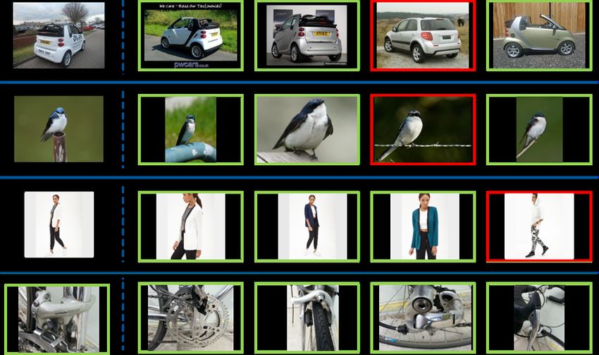
Learning Intra-Batch Connections for Deep Metric Learning

Figure 1. Overview of our proposed approach. Given a mini-batch consisting of N classes, each of them having P images, we initialize the
embedding vectors using a backbone CNN. We then construct a fully connected graph that refines their initial embeddings by performing
K message-passing steps. After each step, the embeddings of the images coming from the same class become more similar to each other
and more dissimilar to the embeddings coming from images that belong to different classes. Finally, we apply Cross-Entropy loss and we
backpropagate the gradients to update the network.

refine their feature representation based on the informa-                • We perform a comprehensive robustness analysis show-
tion taken from their neighbors. More precisely, we use                    ing the stability of our module with respect to the
a convolutional neural network (CNN) to generate feature                   choice of hyperparameters.
embeddings. We then construct a fully connected graph
where each node is represented by the embedding of its                   • We present state-of-the-art results on CUB-200-2011
corresponding sample. In this graph, a series of message                   (Wah et al., 2011), Cars196 (Krause et al., 2013), Stan-
passing steps are performed to update the node embeddings.                 ford online Products (Song et al., 2016) and In-Shop
Not all samples are equally important to predict decision                  Clothes (Liu et al., 2016) datasets.
boundaries, hence, we allow each sample to weigh the im-
portance of neighboring samples by using a dot-product                2. Related Work
self-attention mechanism to compute aggregation weights
for the message passing steps.                                        Metric Learning Losses. Siamese neural networks were
                                                                      first proposed for representation learning in (Bromley et al.,
To draw a parallelism with the triplet loss, our MPN for-             1994). The main idea is to use a CNN to extract a feature
mulation would allow samples to choose their own triplets             representation from an image and using that representation,
which are best to make a prediction on the decision bound-            or embedding, to compare it to other images. In (Chopra
ary. Unlike the triplet loss though, we are not limited to            et al., 2005), the contrastive loss was introduced to train
triplets, as each sample can choose to attend over all other          such a network for face verification. The loss minimizes the
samples in the mini-batch. By training the CNN and MPN                distance between the embeddings of image pairs coming
in an end-to-end manner, we can directly use our CNN                  from the same class and maximizes the distance between
backbone embeddings during inference to perform image                 image pairs coming from different classes. In parallel, re-
retrieval and clustering. While this reaches state-of-the-art         searchers working on convex optimization developed the
results without adding any computational overhead, we also            triplet loss (Schultz & Joachims, 2003; Weinberger & Saul,
show how to further boost the performance by using the                2009) which was later combined with the expressive power
trained MPN at test time, constructing the batches based on           of CNNs, further improving the solutions on face verifica-
k-reciprocal nearest neighbor sampling (Zhong et al., 2017).          tion (Schroff et al., 2015). Triplet loss extends contrastive
Our contribution in this work is three-fold:                          loss by using a triplet of samples consisting of an anchor, a
                                                                      positive, and a negative sample, where the loss is defined
                                                                      to make the distance between the anchor and the positive
   • We propose an approach for deep metric learning that             smaller than the distance between the anchor and the nega-
     computes sample embeddings by taking into account                tive, up to a margin. The concept was later generalized to
     all intra-batch relations. By leveraging message pass-           N-Pair loss (Sohn, 2016), where an anchor and a positive
     ing networks, our method can be trained end-to-end.              sample are compared to N − 1 negative samples at the same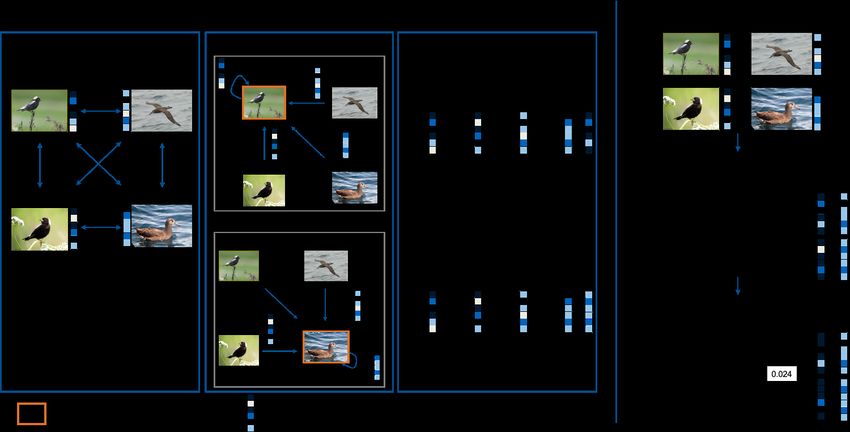
Learning Intra-Batch Connections for Deep Metric Learning

time. In recent years, different approaches based on opti-         learning (Çakir et al., 2019), and person re-identification
mizing other qualities than the distance, such as clustering       (Alemu et al., 2019; Zhao et al., 2019). In metric learning,
(Law et al., 2017; McDaid et al., 2011) or angular distance        SoftTriple loss (Qian et al., 2019) develops a classification
(Wang et al., 2017), have shown to reach good results.             loss where each class is represented by K centers. In the
                                                                   same classification spirit, the Group Loss (Elezi et al., 2020)
Sampling and Ensembles. Since computing the loss of
                                                                   replaces the softmax function with a contextual module that
all possible triplets is computationally infeasible even for
                                                                   considers all the samples in the mini-batch at the same time.
moderately-sized datasets and, furthermore, based on the
knowledge that the majority of them are not informative            Message Passing Networks. Recent works on message
(Schroff et al., 2015), more researchers have given atten-         passing networks (Gilmer et al., 2017) and graph neural net-
tion to intelligent sampling. The work of (Manmatha et al.,        works (Battaglia et al., 2018; Kipf & Welling, 2017) have
2017) showed conclusive evidence that the design of smart          been successfully applied to problems such as human action
sampling strategies is as important as the design of efficient     recognition (Guo et al., 2018), visual question answering
loss functions. In (Ge et al., 2018), the authors propose          (Narasimhan et al., 2018) or tracking (Brasó & Leal-Taixé,
a hierarchical version of triplet loss that embeds the sam-        2020). Given a graph with some initial features for nodes
pling during the training process. More recent techniques          and edges, the main idea behind these models is to embed
continue this line of research by developing new sampling          nodes and edges into representations that take into account
strategies (Duan et al., 2019; Xuan et al., 2020a;b) while         not only the node’s own features but also those of its neigh-
others introduce new loss functions (Wang et al., 2019a;           bors in the graph, as well as the graphs overall topology.
Xu et al., 2019). In parallel, other researchers investigated      The attention-based Transformers (Vaswani et al., 2017;
the usage of ensembles for deep metric learning, unsurpris-        Xu et al., 2015), which can be seen as message passing
ingly finding out that ensembles outperform single networks        networks, have revolutionized the field of natural language
trained on the same loss (Kim et al., 2018; Opitz et al., 2017;    processing, and within the computer vision, have shown
Sanakoyeu et al., 2019; Xuan et al., 2018; Yuan et al., 2017).     impressive results in object detection (Carion et al., 2020).
Global Metric Learning Losses. Most of the mentioned               Closely related to message passing networks, (Elezi et al.,
losses do not consider the global structure of the mini-batch.     2020) considered contextual information for metric learn-
The work of (Movshovitz-Attias et al., 2017) proposes to           ing based on the similarity (dissimilarity) between samples
optimize the triplet loss on a space of triplets different from    coming from the same class (respectively from different
the one of the original samples, consisting of an anchor data      classes). However, they use a handcrafted rule as part of
point and similar and dissimilar learned proxy data points.        their loss function that only considers the label preferences
These proxies approximate the original data points so that         (Elezi et al., 2018). In contrast, based on message passing
a triplet loss over the proxies is a tight upper bound of the      networks, we develop a novel learnable model, where each
loss over the original samples. The introduction of proxies        sample uses learned attention scores to choose the impor-
adds additional contextual knowledge that shows to signif-         tance of its neighbors, and based on this information, refines
icantly improve triplet loss. The results of this approach         its own feature representation.
were significantly improved by using training tricks (Teh
et al., 2020) or generalizing the concept of proxy triplets to     3. Methodology
multiple proxy anchors (Kim et al., 2020; Zhu et al., 2020).
In (Duan et al., 2018) the authors generate negative samples       The goal of the message passing steps is to exchange infor-
in an adversarial manner, while in (Lin et al., 2018) a deep       mation between all samples in the mini-batch and to refine
variational metric learning framework was proposed to ex-          the feature embeddings accordingly. Note that this approach
plicitly model the intra-class variance and disentangle the        is very different from label-propagation methods as used
intra-class invariance. In the work of (Wang et al., 2019b),       in (Elezi et al., 2020), where samples exchange informa-
a non-proxy contextual loss function was developed. The            tion only on their label preferences, information which only
authors propose a loss function based on a ranking distance        implicitly affects the choice of their final feature vectors.
that considers all the samples in the mini-batch
                                                                   In our proposed method, each sample exchanges messages
Classification Losses for Metric Learning. A recent line           with all the other samples in the mini-batch, regardless of
of work (Zhai & Wu, 2019; Zheng et al., 2019) is showing           whether the samples belong to the same class or not. In
that a carefully designed classification loss function can ri-     this way, our method considers both the intra-class and
val, if not outperform, triplet-based functions in metric learn-   inter-class relations between all samples in the mini-batch,
ing. This has already been shown for multiple tasks such as        allowing our network to receive information about the over-
hashing (binary-embedding) (He et al., 2018a), landmark            all structure of the mini-batch. We can use cross-entropy
detection (He et al., 2018b; Revaud et al., 2019), few-shot        loss to train our network since the information of the mini-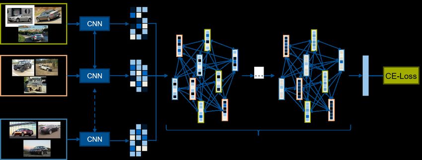
Learning Intra-Batch Connections for Deep Metric Learning

batch is already contained in the refined individual feature     Passing Messages. We apply L message passing steps suc-
embeddings.                                                      cessively. In each step, we pass messages between all sam-
                                                                 ples in a batch and obtain updated features hl+1
                                                                                                                i   of node i
3.1. Overview                                                    at message passing step l + 1 by aggregating the features hlj
                                                                 of all neighbouring nodes j ∈ Ni at message passing step l:
In Figure 1, we show an overview of our proposed approach.
We compute feature vectors for each sample as follows:
                                                                                              X
                                                                                     hl+1
                                                                                       i   =       W l hlj                 (1)
                                                                                              j∈Ni
  1. Generate initial embedding feature vectors using a
     CNN and construct a fully connected graph, where
                                                                 where W l is the corresponding weight matrix of message
     each node represents a sample in the mini-batch.
                                                                 passing step l. As we construct a fully connected graph, the
  2. Perform message-passing between nodes to refine             neighboring nodes Ni consist of all nodes in the given batch,
     the initial embedding feature vectors by utilizing dot-     thus each feature representation of an image is affected by
     product self-attention.                                     all the other images in the mini-batch.

  3. Perform classification and optimize both the MPN and        Attention Weights on the Messages. Not all samples of a
     the backbone CNN in an end-to-end fashion using             mini-batch are equally informative to predict the decision
     cross-entropy loss on the refined node feature vectors.     boundaries between classes. Hence, we add an attention
                                                                 score α to every message passing step (see Figure 2 on Mes-
                                                                 sage Passing) to allow each sample to weigh the importance
3.2. Feature Initialization and Graph Construction
                                                                 of the other samples in the mini-batch:
The global structure of the embedding space is modeled by                                   X
a graph G = (V, E), where V represents the nodes, i.e., all                        hl+1
                                                                                     i   =        l
                                                                                                αij W l hlj              (2)
images in the training dataset, and E the edges connecting                                  j∈Ni
them. An edge represents the importance of one image to
the other, expressed, for example, by their similarity. Dur-     where αij is the attention score between node i and node j.
ing training, we would ideally take the graph of the whole       We utilize dot-product self-attention to compute the atten-
dataset into account, but this is computationally infeasible.    tion scores, leading to αij at step l defined as:
Therefore, we construct mini-batches consisting of n ran-
domly sampled classes with p randomly chosen samples per                           l
                                                                                          W lq hli (W lk hlj )T
class. Each sample in the mini-batch is regarded as a node                        αij =            √                      (3)
                                                                                                     d
in a mini-batch graph GB = (VB , EB ). Unlike CNNs that
perform well on data with an underlying grid-like or Eu-
clidean structure (Bronstein et al., 2017), graphs have a non-   where W lq is the weight matrix corresponding to the receiv-
euclidean structure. Thus, to fully explore the graph-like       ing node and W lk is the weight matrix corresponding to the
structure, we model the mini-batch relations using MPNs.         sending node on message passing step l. Furthermore, we
                                                                 apply the softmax function to all in-going attention scores
More precisely, we use a backbone CNN to compute the             (edges) of a given node i. To allow the MPN to learn a
initial embeddings f ∈ Rd for all samples in a mini-batch,       diverse set of attention scores, we apply M dot product
where d is their embedding dimension. To leverage all            self-attention heads in every message passing step and con-
relations in the batch, we utilize a fully connected graph,      catenate their results. To this end, instead of using single
where every node with initial node features h0i = f is           weight matrices W lq , W lk and W l , we now use different
connected to all the other nodes in the graph (see Figure 2                                      d                  d
                                                                 weight matrices W l,m q   ∈ R M ×d , W l,mk    ∈ R M ×d and
in the upper left corner).                                                    d
                                                                 W l,m ∈ R M ×d for each attention head:
3.3. Message Passing Network
                                                                                 X l,1                    X l,M
In order to refine the initial feature vectors based on the        hl+1
                                                                     i    = cat(     αij W l,1 hlj , ...,    αij W l,M hlj )
                                                                                j∈Ni                     j∈Ni
contextual information of the mini-batch, we use message
                                                                                                                          (4)
passing to exchange information between single nodes, i.e.,
                                                                 where cat represents the concatenation.
between samples of the mini-batch. To this end, we uti-
lize MPNs with graph attention (Velickovic et al., 2018) for     Note, by using the attention-head specific weight matrices,
deep metric learning. It should be noted that the following      we reduce the dimension of all embeddings hlj by M    1
                                                                                                                         so
formulation is equivalent to the Transformers architecture       that when we concatenate the embeddings generated by all
(Vaswani et al., 2017), which can be seen as a fully con-        attention heads the resulting embedding hl+1
                                                                                                           i   has the same
nected graph attention network (Velickovic et al., 2018).        dimension as the input embedding hli .
Learning Intra-Batch Connections for Deep Metric Learning
Figure 2. Left: To update the feature vectors in a message-passing step we first construct a fully connected graph and compute attention
scores between all samples in a batch. We then pass messages between nodes and weigh them with the corresponding attention scores.
During the aggregation step, we sum the weighted messages to get updated node features. Right: Visualization of development of attention
scores and feature vectors over two steps of message passing steps showing that feature vectors, as well as attention scores between
samples from the same class, get more and more similar.
Adding Skip Connections. We add a skip connection to the message passing steps. As the MPN takes its initial
around the attention block (He et al., 2016) and apply layer feature vectors from the backbone CNN, we add an auxil-
normalization (Ba et al., 2016) given by: iary cross-entropy loss to the backbone CNN, to ensure a
sufficiently discriminative initialization. This loss is also
f (hl+1 l+1
i ) = LayerN orm(hi + hli ) (5) needed since at test time we do not use the MPN, as de-
scribed below. Both loss functions utilize label smoothing
where hl+1
i is the outcome of Equation 4. We then apply two and low temperature scaling (Teh et al., 2020; Zhai & Wu,
fully connected layers, followed by another skip connection 2019) to ensure generalized, but discriminative, decision
(He et al., 2016) and a layer normalization (Ba et al., 2016): boundaries.
g(hl+1 l+1 l+1
i ) = LayerN orm(F F (f (hi )) + f (hi )) (6) 3.5. Inference
One disadvantage of using the MPN during inference is
where F F represents the two linear layers. Finally, we
that in order to generate an embedding vector for a sample,
pass the outcome of Equation 6 to the next message passing
we need to create a batch of samples to perform message
step. For illustrative purposes, in Figure 2, we show how
passing as we do during the training. However, using the
the attention scores and the feature vectors evolve over the
MPN during inference would be unfair to other methods
message passing steps. As can be seen, the feature vectors
that directly perform retrieval on the CNN embedding since
of samples of the same class become more and more similar.
we would be adding parameters, hence, expressive power,
Similar to (Velickovic et al., 2018), we indirectly address
to the model. Therefore, we perform all experiments by di-
oversmoothing by applying node-wise attention scores αi,j
rectly using the embedding feature vectors of the backbone
(Equation 3) during the feature aggregation step (Min et al.,
CNN unless stated differently. The intuition is that when
2020).
optimizing the CNN and MPN together in an end-to-end
3.4. Optimization fashion, the CNN features will have also improved with the
information of sample relations. In the ablation studies, we
We apply a fully connected layer on the refined features after
show how the performance can be further improved with
the last message passing step and then use cross-entropy
a simple batch construction strategy at test time. For more
loss. Even if cross-entropy loss itself does not take into
discussion on using MPN at test time, we refer the reader to
account the relations between different samples, this infor-
the supplementary material.
mation is already present in the refined embeddings, thanksLearning Intra-Batch Connections for Deep Metric Learning
4. Experiments consists of 22,634 classes (5 images per class on av-
erage) of product images from ebay. We use 11, 318
In this section, we compare our proposed approach to state- classes for training and the remaining 11, 316 classes
of-the-art deep metric learning approaches on four public for testing.
benchmarks. To underline the effectiveness of our approach,
we further present an extensive ablation study. • In-Shop Clothes (Liu et al., 2016) contains 7, 982
4.1. Implementation Details classes of clothing items, with each class having 4
images on average. We use 3, 997 classes for training,
We implement our method in PyTorch (Paszke et al., 2017) while the test set, containing 3, 985 classes, is split into
library. Following other works (Brattoli et al., 2019; Çakir a query set and a gallery set.
et al., 2019; Manmatha et al., 2017; Sanakoyeu et al., 2019;
Teh et al., 2020; Xuan et al., 2020b; Zhai & Wu, 2019), we
present results using ResNet50 (He et al., 2016) pretrained Evaluation Metrics: For evaluation, we use the two com-
on ILSVRC 2012-CLS dataset (Russakovsky et al., 2015) monly used evaluation metrics, Recall@K (R@K) (Jégou
as backbone CNN. Like the majority of recent methods et al., 2011) and Normalized Mutual Information (NMI)
(Ge et al., 2018; Kim et al., 2020; Park et al., 2019; Qian (McDaid et al., 2011). The first one evaluates the retrieval
et al., 2019; Wang et al., 2019a;b; Zhu et al., 2020), we use performance by computing the percentage of images whose
embedding dimension of sizes 512 for all our experiments K nearest neighbors contain at least one sample of the same
and low temperature scaling for the softmax cross-entropy class as the query image. To evaluate the clustering qual-
loss function (Guo et al., 2017). Furthermore, we preprocess ity, we apply K-means clustering (MacQueen, 1967) on
the images following (Kim et al., 2020). We resize the the embedding feature vectors of all test samples, and com-
cropped image to 227×227, followed by applying a random pute NMI based on this clustering. To be more specific,
horizontal flip. During test time, we resize the images to NMI evaluates how much the knowledge about the ground
256 × 256 and take a center crop of size 227 × 227. We truth classes increases given the clustering obtained by the
train all networks for 70 epochs using RAdam optimizer K-means algorithm.
(Liu et al., 2020). To find all hyperparameters we perform
random search (Bergstra & Bengio, 2012). For mini-batch 4.3. Comparison to state-of-the-art
construction, we first randomly sample a given number of Quantitative Results. In Table 1, we present the results
classes, followed by randomly sampling a given number of of our method and compare them with the results of other
images for each class as commonly done in metric learning approaches on CUB-200-2011 (Wah et al., 2011), Cars196
(Elezi et al., 2020; Schroff et al., 2015; Teh et al., 2020; (Krause et al., 2013), and Stanford Online Products (Song
Zhai & Wu, 2019). We use small mini-batches of size et al., 2016). On CUB-200-2011 dataset, our method
50-100 and provide an analysis on different numbers of reaches 70.3 Recall@1, an improvement of 0.6 percent-
classes and samples on CUB-200-2011 and Cars196 in the age points (pp) over the state-of-the-art Proxy Anchor (Kim
supplementary. Our forward pass takes 73% of time for the et al., 2020) using ResNet50 backbone. On the NMI metric,
backbone and the remaining for the MPN. All the training we outperform the highest scoring method, DiVA (Milbich
is done in a single TitanX GPU, i.e., the method is memory et al., 2020) by 2.6pp. On Cars196, we reach 88.1 Recall@1,
efficient. an improvement of 0.4pp over Proxy Anchor (Kim et al.,
4.2. Benchmark Datasets and Evaluation Metrics 2020) with ResNet50 backbone. On the same dataset, we
reach 74.8 on the NMI score, 0.8pp higher than the previous
Datasets: We conduct experiments on 4 publicly available best-performing method, Normalized Softmax (Zhai & Wu,
datasets using the conventional splitting protocols (Song 2019). On Stanford Online Products dataset, our method
et al., 2016): reaches 81.4 Recall@1 which is 1.3pp better than the previ-
ous best method, HORDE (Jacob et al., 2019). On the NMI
• CUB-200-2011 (Wah et al., 2011) consists of 200 metric, our method reaches the highest score, outperforming
classes of birds with each class containing 58 images SoftTriple Loss (Qian et al., 2019) by 0.6pp.
on average. For training, we use the first 100 classes
and for testing the remaining classes. Finally, we present the results of our method on the In-
Shop Clothes dataset in Table 2. Our method reaches 92.8
• Cars196 (Krause et al., 2013) contains 196 classes Recall@1, an improvement of 0.7pp over the previous best
representing different cars with each class containing method Proxy Anchor (Kim et al., 2020) with ResNet50
on average 82 images. We use the first 98 classes for backbone. In summary, while in the past, different methods
training and the remaining classes for testing. (Proxy Anchor (Kim et al., 2020), ProxyNCA++ (Teh et al.,
2020), Normalized Softmax (Zhai & Wu, 2019), HORDE
• Stanford Online Products (SOP) (Song et al., 2016) (Jacob et al., 2019), SoftTriple Loss (Qian et al., 2019),Learning Intra-Batch Connections for Deep Metric Learning
CUB-200-2011 CARS196 Stanford Online Products
Method BB R@1 R@2 R@4 R@8 NMI R@1 R@2 R@4 R@8 NMI R@1 R@10 R@100 NMI
Triplet64 (Schroff et al., 2015) CVPR15 G 42.5 55 66.4 77.2 55.3 51.5 63.8 73.5 82.4 53.4 66.7 82.4 91.9 89.5
Npairs64 (Sohn, 2016) NeurIPS16 G 51.9 64.3 74.9 83.2 60.2 68.9 78.9 85.8 90.9 62.7 66.4 82.9 92.1 87.9
Deep Spectral512 (Law et al., 2017) ICML17 BNI 53.2 66.1 76.7 85.2 59.2 73.1 82.2 89.0 93.0 64.3 67.6 83.7 93.3 89.4
Angular Loss512 (Wang et al., 2017) ICCV17 G 54.7 66.3 76 83.9 61.1 71.4 81.4 87.5 92.1 63.2 70.9 85.0 93.5 88.6
Proxy-NCA64 (Movshovitz-Attias et al., 2017) ICCV17 BNI 49.2 61.9 67.9 72.4 59.5 73.2 82.4 86.4 88.7 64.9 73.7 - - 90.6
Margin Loss128 (Manmatha et al., 2017) ICCV17 R50 63.6 74.4 83.1 90.0 69.0 79.6 86.5 91.9 95.1 69.1 72.7 86.2 93.8 90.7
Hierarchical triplet512 (Ge et al., 2018) ECCV18 BNI 57.1 68.8 78.7 86.5 - 81.4 88.0 92.7 95.7 - 74.8 88.3 94.8 -
ABE512 (Kim et al., 2018) ECCV18 G 60.6 71.5 79.8 87.4 - 85.2 90.5 94.0 96.1 - 76.3 88.4 94.8 -
Normalized Softmax512 (Zhai & Wu, 2019) BMVC19 R50 61.3 73.9 83.5 90.0 69.7 84.2 90.4 94.4 96.9 74.0 78.2 90.6 96.2 91.0
RLL-H512 (Wang et al., 2019b) CVPR19 BNI 57.4 69.7 79.2 86.9 63.6 74 83.6 90.1 94.1 65.4 76.1 89.1 95.4 89.7
Multi-similarity512 (Wang et al., 2019a) CVPR19 BNI 65.7 77.0 86.3 91.2 - 84.1 90.4 94.0 96.5 - 78.2 90.5 96.0 -
Relational Knowledge512 (Park et al., 2019) CVPR19 G 61.4 73.0 81.9 89.0 - 82.3 89.8 94.2 96.6 - 75.1 88.3 95.2 -
Divide and Conquer1028 (Sanakoyeu et al., 2019) CVPR19 R50 65.9 76.6 84.4 90.6 69.6 84.6 90.7 94.1 96.5 70.3 75.9 88.4 94.9 90.2
SoftTriple Loss512 (Qian et al., 2019) ICCV19 BNI 65.4 76.4 84.5 90.4 69.3 84.5 90.7 94.5 96.9 70.1 78.3 90.3 95.9 92.0
HORDE512 (Jacob et al., 2019) ICCV19 BNI 66.3 76.7 84.7 90.6 - 83.9 90.3 94.1 96.3 - 80.1 91.3 96.2 -
MIC128 (Brattoli et al., 2019) ICCV19 R50 66.1 76.8 85.6 - 69.7 82.6 89.1 93.2 - 68.4 77.2 89.4 95.6 90.0
Easy triplet mining512 (Xuan et al., 2020b) WACV20 R50 64.9 75.3 83.5 - - 82.7 89.3 93.0 - - 78.3 90.7 96.3 -
Group Loss1024 (Elezi et al., 2020) ECCV20 BNI 65.5 77.0 85.0 91.3 69.0 85.6 91.2 94.9 97.0 72.7 75.1 87.5 94.2 90.8
Proxy NCA++512 (Teh et al., 2020) ECCV20 R50 66.3 77.8 87.7 91.3 71.3 84.9 90.6 94.9 97.2 71.5 79.8 91.4 96.4 -
DiVA512 (Milbich et al., 2020) ECCV20 R50 69.2 79.3 - - 71.4 87.6 92.9 - - 72.2 79.6 - - 90.6
PADS128 (Roth et al., 2020) CVPR20 R50 67.3 78.0 85.9 - 69.9 83.5 89.7 93.8 - 68.8 76.5 89.0 95.4 89.9
Proxy Anchor512 (Kim et al., 2020) CVPR20 BNI 68.4 79.2 86.8 91.6 - 86.1 91.7 95.0 97.3 - 79.1 90.8 96.2 -
Proxy Anchor512 (Kim et al., 2020) CVPR20 R50 69.7 80.0 87.0 92.4 - 87.7 92.9 95.8 97.9 - 80.0 91.7 96.6 -
Proxy Few512 (Zhu et al., 2020) NeurIPS20 BNI 66.6 77.6 86.4 - 69.8 85.5 91.8 95.3 - 72.4 78.0 90.6 96.2 90.2
Ours512 R50 70.3 80.3 87.6 92.7 74.0 88.1 93.3 96.2 98.2 74.8 81.4 91.3 95.9 92.6
Table 1. Retrieval and Clustering performance on CUB-200-2011, CARS196 and Stanford Online Products datasets. Bold indicates
best, red second best, and blue third best results. The exponents attached to the method name indicates the embedding dimension.
BB=backbone, G=GoogLeNet, BNI=BN-Inception and R50=ResNet50.
Method BB R@1 R@10 R@20 R@40 ments by training the backbone CNN solely with the auxil-
FashionNet4096 (Liu et al., 2016) CVPR16 V 53.0 73.0 76.0 79.0
A-BIER512 (Opitz et al., 2020) PAMI20 G 83.1 95.1 96.9 97.8 iary loss, i.e., the cross-entropy loss on the backbone CNN,
ABE512 (Kim et al., 2018) ECCV18 G 87.3 96.7 97.9 98.5
Multi-similarity512 (Wang et al., 2019a) CVPR19 BNI 89.7 97.9 98.5 99.1
and without MPN (see the first row in Table 3). For a fair
Learning to Rank512 (Çakir et al., 2019) R50 90.9 97.7 98.5 98.9 comparison, we use the same implementation details as for
HORDE512 (Jacob et al., 2019) ICCV19 BNI 90.4 97.8 98.4 98.9
MIC128 (Brattoli et al., 2019) ICCV19 R50 88.2 97.0 98.0 98.8
the training with MPN. On CUB-200-2011, this leads to a
Proxy NCA++512 (Teh et al., 2020) ECCV20 R50 90.4 98.1 98.8 99.2 performance drop of 2.8pp in Recall@1 (to 67.5) and 4.2pp
Proxy Anchor512 (Kim et al., 2020) CVPR20 BNI 91.5 98.1 98.8 99.1
Proxy Anchor512 (Kim et al., 2020) CVPR20 R50 92.1 98.1 98.7 99.2 in NMI (to 69.8). On Cars196, it leads to a more signifi-
Ours512 R50 92.8 98.5 99.1 99.2 cant performance drop of 3.9pp in Recall@1 (to 84.2) and
6.1pp in NMI (to 68.7), showing the benefit of our proposed
Table 2. Retrieval performance on In Shop Clothes. formulation.
DiVA (Milbich et al., 2020)) scored the highest in at-least To give an intuition of how the MPN evolves during the
one metric, now our method reaches the best results in all training process, we use GradCam (Selvaraju et al., 2020) to
Recall@1 and NMI metrics across all four datasets. observe which neighbors a sample relies on when computing
the final class prediction after the MPN (Selvaraju et al.,
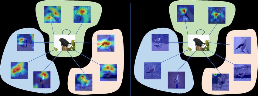
Qualitative Results. In Figure 6, we present qualitative 2020). To do so, we compare the predictions of an untrained
results on the retrieval task for all four datasets. In all MPN to a trained one. As can be seen in the left part of
cases, the query image is given on the left, with the four Figure 7, the untrained MPN takes information from nearly
nearest neighbors given on the right. Green boxes indicate all samples in the batch into account, where red, blue, and
cases where the retrieved image is of the same class as the green represent different classes. The trained MPN (left part
query image, and red boxes indicate a different class. In of Figure 7) only relies on the information of samples of
supplementary material, we provide qualitative evaluations the same class. This suggests that using the MPN with self-
on the clustering performance using t-SNE (van der Maaten attention scores as edge weights enforces the embeddings
& Hinton, 2012) visualization. of negative and positive samples to become more dissimilar
4.4. Ablation Studies and Robustness Analysis and similar, respectively. In supplementary, we also provide
and compare visualizations of the embedding vectors of a
In this section, we use the CUB-200-2011 (Wah et al., 2011) batch of samples after one epoch of training and of all test
and Cars196 (Krause et al., 2013) datasets to analyze the samples after the whole training.
robustness of our method and show the importance of our
Number of Message Passing Steps and Attention Heads.
design choices.
In Figure 3, we investigate the robustness of the algorithm
MPN Matters. To show the performance improvement when we differ the number of message passing steps and
when using the MPN during training, we conduct experi-Learning Intra-Batch Connections for Deep Metric Learning
Figure 5. Performance for different embed-
Figure 3. Relative difference to the best model Figure 4. Relative difference to the best ding dimensions on CUB-200-2011 and
with respect to Recall@1 on CUB-200-2011. model with respect to Recall@1 on Cars196. Cars196.
Figure 7. Comparison of the embeddings of a given batch after one
epoch of training without and with MPN.
Figure 6. Retrieval results on a set of images from CUB-200-2011
(top), Cars196 (second from top), Stanford Online Products (sec- drop in performance when the size of the embedding layer
ond from bottom), and In-Shop Clothes (bottom) datasets using our
gets bigger than 512. While increasing the dimension of the
model. The most left column contains query images and the results
embedding layer results in even better performance, for fair-
are ranked by distance. Green frames indicate that the retrieved
image is from the same class as the query image, while red frames ness with the other methods that do not use an embedding
indicate that the retrieved image is from a different class. size larger than 512, we avoid those comparisons.
Auxiliary Loss Function. Considering that in the default
attention heads of our MPN. On CUB-200-2011 dataset, scenario, we do not use the MPN during inference, we in-
we reach the best results when we use a single message vestigate the effect of adding the auxiliary loss function at
passing step, containing two attention heads. We see that the top of the backbone CNN embedding layer. On CUB-
increasing the number of message passing steps or the num- 200-2011 dataset, we see that such a loss helps the network
ber of attention heads, for the most part, does not result in improve by 2.2pp in Recall@1. Without the loss, the perfor-
a large drop in performance. The biggest drop in perfor- mance of the network drops to 68.1 as shown in the second
mance happens when we use four message-passing steps, row of Table 3. On the other hand, removing the auxiliary
each having sixteen attention heads. In Figure 4, we do a loss function leads to a performance drop of only 0.9pp in
similar robustness analysis for the Cars196 dataset. Unlike Recall@1 on Cars196 to 87.2. However, the NMI perfor-
CUB-200-2011, the method performs best using two layers mance drops by 2.7pp to 72.1 on Cars196 and 2.0pp on
and eight attention heads. However, it again performs worst CUB-200-2011.
using four message passing steps. This observation is in
Implicit Regularization. We further investigate the train-
line with (Velickovic et al., 2018), which also utilizes a few
ing behavior of our proposed approach on CUB-200-2011.
message passing steps when applying graph attention.
As already stated above, Group Loss (Elezi et al., 2020) also
Embedding Dimension. In Figure 5, we measure the per- utilized contextual classification, with the authors claim-
formance of the model as a function of the embedding size. ing that it introduces implicit regularization and thus less
We observe that the performance of the network increases overfitting. However, their approach is based on a hand-
on both datasets when we increase the size of the embedding crafted label propagation rule, while ours takes into account
layer. This is unlike (Wang et al., 2019a), which reports a the contextual information in an end-to-end learnable way.Learning Intra-Batch Connections for Deep Metric Learning
Therefore, we present the training behavior of our approach by simply concatenating the features of k independently
and compare it to the behavior of the Group Loss (Elezi trained networks. Similarly, we also conduct experiments
et al., 2020). As can be seen in Figure 8, Group Loss (Elezi on ensembles using 2 and 5 networks, respectively, and
et al., 2020) shows higher overfitting on the training data, compare our ensemble with that of (Elezi et al., 2020).
while our method is capable of better generalization on the
CUB-200-2011 Cars196 Stanford Online Products In-Shop Clothes
test dataset and has a smaller gap between training and R@1 NMI R@1 NMI R@1 NMI R@1
test performance. We argue that by taking into account the GL 65.5 69.0 85.6 72.7 75.7 91.1 -
Ours 70.3 74.0 88.1 74.8 81.4 92.6 92.8
global structure of the dataset in an end-to-end learnable GL 2 65.8 68.5 86.2 72.6 75.9 91.1 -
way, our approach is able to induce an even stronger implicit Ours 2 72.2 74.3 90.9 74.9 81.8 92.7 92.9
GL 5 66.9 70.0 88.0 74.2 76.3 91.1 -
regularization. Ours 5 73.1 74.4 91.5 75.4 82.1 92.8 93.4
Table 4. Performance of our ensembles and comparisons with the
ensemble models of (Elezi et al., 2020).
In Table 4, we present the results of our ensembles. We see
that when we use 2 networks, the performance increases by
1.9pp on CUB-200-2011, 3.0pp on Cars196, and 0.4pp on
Stanford Online Products. Similarly, the NMI score also
improves by 0.3pp on CUB-200-2011, 0.1pp on Cars196,
and 0.1pp on Stanford Online Products. Unfortunately, the
Recall@1 performance on In-Shop Clothes only improves
Figure 8. Performance on training and test data of CUB-200-2011 by 0.1pp. Using 5 networks, the performance increases
compared to Group Loss (Elezi et al., 2020). by 2.8pp on CUB-200-2011, 3.4pp on Cars196, 0.7pp on
Stanford Online Products, and 0.6pp on In-Shop Clothes
compared to using a single network. NMI on CUB-200-
Using MPN During Test Time. In Table 3, we analyze 2011 is improved by 0.4pp compared to a single network,
the effect of applying message passing during inference on Cars196 it increases by 0.6pp more and on Stanford
(see row four). On CUB-200-2011 dataset, we improve Online Products it increases by 0.6pp.
by 0.5pp in Recall@1, and by 0.5pp on the NMI metric.
Compared to (Elezi et al., 2020), the performance increase
On Cars196 dataset, we also gain 0.5pp in Recall@1 by
of our approach from one network to an ensemble is higher.
using MPN during inference. More impressively, we gain
This is surprising, considering that our network starts from
1.4pp in the NMI metric, putting our results 2.2pp higher
a higher point, and has less room for improvement.
than Normalized Softmax (Zhai & Wu, 2019). We gain an
improvement in performance in all cases, at the cost of extra
parameters. 5. Conclusions
Note, our method does not require the usage of these ex-
tra parameters in inference. As we have shown, for a fair In this work, we propose a model that utilizes the power
comparison, our method reaches state-of-the-art results even of message passing networks for the task of deep metric
without using MPN during inference (see Tables 1 and 2). learning. Unlike classical metric learning methods, e.g.,
We consider the usage of MPN during inference a perfor- triplet loss, our model utilizes all the intra-batch relations in
mance boost, but not a central part of our work. the mini-batch to promote similar embeddings for images
coming from the same class, and dissimilar embeddings
Training Losses Test Time Embeddings
CUB-200-2011
R@1 NMI
CARS196
R@1 NMI
for samples coming from different classes. Our model is
Cross-Entropy Backbone Embeddings 67.5 69.8 84.2 68.7 fully learnable, end-to-end trainable, and does not utilize any
MPN Loss Backbone Embeddings 68.1 72.0 87.2 72.1
MPN Loss + Auxiliary Loss Backbone Embeddings 70.3 74.0 88.1 74.8 handcrafted rules. Furthermore, our model achieves state-of-
MPN Loss + Auxiliary Loss MPN Embeddings 70.8 74.5 88.6 76.2
the-art results while using the same number of parameters,
and compute time, during inference. In future work, we will
Table 3. Performance of the network with and without MPN during explore the applicability of our model for the tasks of semi-
training and testing time. We achieved all results using embedding supervised deep metric learning and deep metric learning in
dimension 512.
the presence of only relative labels.
Ensembles. The Group Loss (Elezi et al., 2020) showed Acknowledgements. This research was partially funded by
that the performance of their method significantly improves the Humboldt Foundation through the Sofia Kovalevskaja
by using an ensemble at test time. The ensemble was built Award. We thank Guillem Brasó for useful discussions.Learning Intra-Batch Connections for Deep Metric Learning
References Duan, Y., Chen, L., Lu, J., and Zhou, J. Deep embed-
ding learning with discriminative sampling policy. In
Alemu, L. T., Shah, M., and Pelillo, M. Deep constrained
Conference on Computer Vision and Pattern Recognition
dominant sets for person re-identification. In Interna-
(CVPR), 2019.
tional Conference on Computer Vision (ICCV), 2019.
Ba, L. J., Kiros, J. R., and Hinton, G. E. Layer normalization. Elezi, I., Torcinovich, A., Vascon, S., and Pelillo, M. Trans-
CoRR, abs/1607.06450, 2016. ductive label augmentation for improved deep network
learning. In International Conference on Pattern Recog-
Battaglia, P. W., Hamrick, J. B., Bapst, V., Sanchez- nition (ICPR), 2018.
Gonzalez, A., Zambaldi, V. F., Malinowski, M., Tacchetti,
A., Raposo, D., Santoro, A., Faulkner, R., Gülçehre, Elezi, I., Vascon, S., Torchinovich, A., Pelillo, M., and Leal-
Ç., Song, H. F., Ballard, A. J., Gilmer, J., Dahl, G. E., Taixé, L. The group loss for deep metric learning. In
Vaswani, A., Allen, K. R., Nash, C., Langston, V., Dyer, European Conference in Computer Vision (ECCV), 2020.
C., Heess, N., Wierstra, D., Kohli, P., Botvinick, M.,
Vinyals, O., Li, Y., and Pascanu, R. Relational induc- Ge, W., Huang, W., Dong, D., and Scott, M. R. Deep
tive biases, deep learning, and graph networks. CoRR, metric learning with hierarchical triplet loss. In European
abs/1806.01261, 2018. Conference in Computer Vision (ECCV), 2018.
Bergstra, J. and Bengio, Y. Random search for hyper- Gilmer, J., Schoenholz, S. S., Riley, P. F., Vinyals, O., and
parameter optimization. Journal of Machine Learning Dahl, G. E. Neural message passing for quantum chem-
Research (JMLR), 13:281–305, 2012. istry. In International Conference on Machine Learning
(ICML), 2017.
Brasó, G. and Leal-Taixé, L. Learning a neural solver for
multiple object tracking. In Conference on Computer Guo, C., Pleiss, G., Sun, Y., and Weinberger, K. Q. On
Vision and Pattern Recognition (CVPR), 2020. calibration of modern neural networks. In International
Conference on Machine Learning (ICML), 2017.
Brattoli, B., Roth, K., and Ommer, B. MIC: mining in-
terclass characteristics for improved metric learning. In Guo, M., Chou, E., Huang, D., Song, S., Yeung, S., and Fei-
International Conference on Computer Vision (ICCV), Fei, L. Neural graph matching networks for fewshot 3d
2019. action recognition. In European Conference on Computer
Vision (ECCV), 2018.
Bromley, J., Guyon, I., LeCun, Y., Säckinger, E., and Shah,
R. Signature verification using a” siamese” time delay He, K., Zhang, X., Ren, S., and ian Sun, J. Deep residual
neural network. In Advances in Neural Information Pro- learning for image recognition. In 2016 IEEE Conference
cessing Systems (NIPS), 1994. on Computer Vision and Pattern Recognition (CVPR),
Bronstein, M. M., Bruna, J., LeCun, Y., Szlam, A., and Van- 2016.
dergheynst, P. Geometric deep learning: Going beyond He, K., Çakir, F., Bargal, S. A., and Sclaroff, S. Hashing as
euclidean data. IEEE Signal Processing Magazine, 34(4): tie-aware learning to rank. In Conference on Computer
18–42, 2017. Vision and Pattern Recognition (CVPR), 2018a.
Çakir, F., He, K., Xia, X., Kulis, B., and Sclaroff, S. Deep
He, K., Lu, Y., and Sclaroff, S. Local descriptors optimized
metric learning to rank. In Conference on Computer
for average precision. In Conference on Computer Vision
Vision and Pattern Recognition (CVPR), 2019.
and Pattern Recognition, (CVPR), 2018b.
Carion, N., Massa, F., Synnaeve, G., Usunier, N., Kirillov,
A., and Zagoruyko, S. End-to-end object detection with Jacob, P., Picard, D., Histace, A., and Klein, E. Metric
transformers. In European Conference on Computer Vi- learning with HORDE: high-order regularizer for deep
sion (ECCV), 2020. embeddings. In International Conference on Computer
Vision (ICCV), 2019.
Chopra, S., Hadsell, R., and LeCun, Y. Learning a similarity
metric discriminatively, with application to face verifi- Jégou, H., Douze, M., and Schmid, C. Product quantization
cation. In Conference on Computer Vision and Pattern for nearest neighbor search. IEEE Trans. Pattern Anal.
Recognition (CVPR), 2005. Mach. Intell. (tPAMI), 33(1):117–128, 2011.
Duan, Y., Zheng, W., Lin, X., Lu, J., and Zhou, J. Deep Kim, S., Kim, D., Cho, M., and Kwak, S. Proxy anchor loss
adversarial metric learning. In Conference on Computer for deep metric learning. In Conference on Computer
Vision and Pattern Recognition (CVPR), 2018. Vision and Pattern Recognition (CVPR), 2020.Learning Intra-Batch Connections for Deep Metric Learning
Kim, W., Goyal, B., Chawla, K., Lee, J., and Kwon, K. Narasimhan, M., Lazebnik, S., and Schwing, A. G. Out
Attention-based ensemble for deep metric learning. In of the box: Reasoning with graph convolution nets for
European Conference on Computer Vision (ECCV), 2018. factual visual question answering. In Advances in Neural
Information Processing Systems (NeurIPS), 2018.
Kipf, T. N. and Welling, M. Semi-supervised classifica-
tion with graph convolutional networks. In International Opitz, M., Waltner, G., Possegger, H., and Bischof, H. BIER
Conference on Learning Representations (ICLR), 2017. - boosting independent embeddings robustly. In Interna-
tional Conference on Computer Vision (ICCV), 2017.
Krause, J., Stark, M., Deng, J., and Fei-Fei, L. 3d object
representations for fine-grained categorization. In In- Opitz, M., Waltner, G., Possegger, H., and Bischof, H. Deep
ternational IEEE Workshop on 3D Representation and metric learning with BIER: boosting independent embed-
Recognition, 2013. dings robustly. IEEE Trans. Pattern Anal. Mach. Intell.
(tPAMI), 42(2):276–290, 2020.
Law, M. T., Urtasun, R., and Zemel, R. S. Deep spectral
clustering learning. In Proceedings of the 34th Interna- Park, W., Kim, D., Lu, Y., and Cho, M. Relational knowl-
tional Conference on Machine Learning (ICML), 2017. edge distillation. In Conference on Computer Vision and
Pattern Recognition (CVPR), 2019.
Lin, X., Duan, Y., Dong, Q., Lu, J., and Zhou, J. Deep
variational metric learning. In European Conference in Paszke, A., Gross, S., Chintala, S., Chanan, G., Yang, E.,
Computer Vision (ECCV), 2018. DeVito, Z., Lin, Z., Desmaison, A., Antiga, L., and Lerer,
A. Automatic differentiation in pytorch. NIPS Workshops,
Liu, L., Jiang, H., He, P., Chen, W., Liu, X., Gao, J., and
2017.
Han, J. On the variance of the adaptive learning rate
and beyond. In International Conference on Learning Qian, Q., Shang, L., Sun, B., Hu, J., Tacoma, T., Li, H.,
Representations (ICLR), 2020. and Jin, R. Softtriple loss: Deep metric learning without
triplet sampling. In International Conference on Com-
Liu, Z., Luo, P., Qiu, S., Wang, X., and Tang, X. Deepfash-
puter Vision (ICCV), 2019.
ion: Powering robust clothes recognition and retrieval
with rich annotations. In Conference on Computer Vision
Revaud, J., Almazán, J., Rezende, R. S., and de Souza,
and Pattern Recognition, (CVPR), 2016.
C. R. Learning with average precision: Training image
MacQueen, J. Some methods for classification and analysis retrieval with a listwise loss. In International Conference
of multivariate observations. In Proc. Fifth Berkeley Symp. on Computer Vision (ICCV), 2019.
on Math. Statist. and Prob., Vol. 1, pp. 281–297, 1967.
Roth, K., Milbich, T., and Ommer, B. PADS: policy-adapted
Manmatha, R., Wu, C., Smola, A. J., and Krähenbühl, P. sampling for visual similarity learning. In Conference on
Sampling matters in deep embedding learning. In Inter- Computer Vision and Pattern Recognition (CVPR), 2020.
national Conference on Computer Vision (ICCV), 2017.
Russakovsky, O., Deng, J., Su, H., Krause, J., Satheesh, S.,
McDaid, A. F., Greene, D., and Hurley, N. J. Normalized Ma, S., Huang, Z., Karpathy, A., Khosla, A., Bernstein,
mutual information to evaluate overlapping community M. S., Berg, A. C., and Li, F. Imagenet large scale visual
finding algorithms. CoRR, abs/1110.2515, 2011. recognition challenge. Int. J. Comput. Vis. (IJCV), 115
(3):211–252, 2015.
Milbich, T., Roth, K., Bharadhwaj, H., Sinha, S., Bengio,
Y., Ommer, B., and Cohen, J. P. Diva: Diverse visual Sanakoyeu, A., Tschernezki, V., Büchler, U., and Ommer,
feature aggregation for deep metric learning. In European B. Divide and conquer the embedding space for metric
Conference in Computer Vision (ECCV), 2020. learning. In Conference on Computer Vision and Pattern
Recognition (CVPR), 2019.
Min, Y., Wenkel, F., and Wolf, G. Scattering GCN: over-
coming oversmoothness in graph convolutional networks. Schroff, F., Kalenichenko, D., and Philbin, J. Facenet: A
In Advances in Neural Information Processing Systems unified embedding for face recognition and clustering. In
(NeurIPS), 2020. Conference on Computer Vision and Pattern Recognition
(CVPR), 2015.
Movshovitz-Attias, Y., Toshev, A., Leung, T. K., Ioffe, S.,
and Singh, S. No fuss distance metric learning using Schultz, M. and Joachims, T. Learning a distance metric
proxies. In International Conference on Computer Vision from relative comparisons. In Advances in Neural Infor-
(ICCV), 2017. mation Processing Systems (NIPS), 2003.Learning Intra-Batch Connections for Deep Metric Learning
Selvaraju, R. R., Cogswell, M., Das, A., Vedantam, R., Xu, K., Ba, J., Kiros, R., Cho, K., Courville, A. C., Salakhut-
Parikh, D., and Batra, D. Grad-cam: Visual explanations dinov, R., Zemel, R. S., and Bengio, Y. Show, attend and
from deep networks via gradient-based localization. Int. tell: Neural image caption generation with visual atten-
J. Comput. Vis. (IJCV), 128(2):336–359, 2020. tion. In International Conference on Machine Learning
(ICML), 2015.
Sohn, K. Improved deep metric learning with multi-class
n-pair loss objective. In Advances in Neural Information Xu, X., Yang, Y., Deng, C., and Zheng, F. Deep asym-
Processing Systems (NIPS), 2016. metric metric learning via rich relationship mining. In
Conference on Computer Vision and Pattern Recognition
Song, H. O., Xiang, Y., Jegelka, S., and Savarese, S. Deep (CVPR), 2019.
metric learning via lifted structured feature embedding. In
Conference on Computer Vision and Pattern Recognition Xuan, H., Souvenir, R., and Pless, R. Deep randomized
(CVPR), 2016. ensembles for metric learning. In European Conference
Computer Vision (ECCV), 2018.
Teh, E. W., DeVries, T., and Taylor, G. W. Proxynca++: Re-
Xuan, H., Stylianou, A., Liu, X., and Pless, R. Hard negative
visiting and revitalizing proxy neighborhood component
examples are hard, but useful. In European Conference
analysis. In European Conference on Computer Vision
in Computer Vision (ECCV), 2020a.
(ECCV), 2020.
Xuan, H., Stylianou, A., and Pless, R. Improved embeddings
van der Maaten, L. and Hinton, G. E. Visualizing non-metric with easy positive triplet mining. In Winter Conference
similarities in multiple maps. Machine Learning, 87(1): on Applications of Computer Vision (WACV), 2020b.
33–55, 2012.
Yuan, Y., Yang, K., and Zhang, C. Hard-aware deeply
Vaswani, A., Shazeer, N., Parmar, N., Uszkoreit, J., Jones, cascaded embedding. In International Conference on
L., Gomez, A. N., Kaiser, L., and Polosukhin, I. Atten- Computer Vision (ICCV), 2017.
tion is all you need. In Advances in Neural Information
Processing Systems (NIPS), 2017. Zhai, A. and Wu, H. Classification is a strong baseline for
deep metric learning. In British Machine Vision Confer-
Velickovic, P., Cucurull, G., Casanova, A., Romero, A., ence (BMVC), 2019.
Liò, P., and Bengio, Y. Graph attention networks. In
Zhang, X., Zhou, F., Lin, Y., and Zhang, S. Embedding
International Conference on Learning Representations
label structures for fine-grained feature representation. In
(ICLR), 2018.
Conference on Computer Vision and Pattern Recognition
Wah, C., Branson, S., Welinder, P., Perona, P., and Belongie, (CVPR), 2016.
S. The Caltech-UCSD Birds-200-2011 Dataset. Tech- Zhao, K., Xu, J., and Cheng, M. Regularface: Deep face
nical Report CNS-TR-2011-001, California Institute of recognition via exclusive regularization. In Conference
Technology, 2011. on Computer Vision and Pattern Recognition (CVPR),
2019.
Wang, J., Zhou, F., Wen, S., Liu, X., and Lin, Y. Deep metric
learning with angular loss. In International Conference Zheng, X., Ji, R., Sun, X., Zhang, B., Wu, Y., and Huang,
on Computer Vision (ICCV), 2017. F. Towards optimal fine grained retrieval via decorrelated
centralized loss with normalize-scale layer. In Conference
Wang, X., Han, X., Huang, W., Dong, D., and Scott, M. R. on Artificial Intelligence (AAAI), 2019.
Multi-similarity loss with general pair weighting for deep
metric learning. In Conference on Computer Vision and Zhong, Z., Zheng, L., Cao, D., and Li, S. Re-ranking
Pattern Recognition (CVPR), 2019a. person re-identification with k-reciprocal encoding. In
Conference on Computer Vision and Pattern Recognition
Wang, X., Hua, Y., Kodirov, E., Hu, G., Garnier, R., and (CVPR), 2017.
Robertson, N. M. Ranked list loss for deep metric learn-
ing. In Conference on Computer Vision and Pattern Zhu, Y., Yang, M., Deng, C., and Liu, W. Fewer is more:
Recognition (CVPR), 2019b. A deep graph metric learning perspective using fewer
proxies. In Advances in Neural Information Processing
Weinberger, K. Q. and Saul, L. K. Distance metric learning Systems (NeurIPS), 2020.
for large margin nearest neighbor classification. Jour-
nal of Machine Learning Research (JMLR), 10:207–244,
2009.You can also read