ON THE EFFICACY OF COMPACT RADAR TRANSPONDERS FOR INSAR GEODESY: RESULTS OF MULTI-YEAR FIELD TESTS
←
→
Page content transcription
If your browser does not render page correctly, please read the page content below
CZIKHARDT ET AL., JUN 2021, SUBMITTED TO IEEE TRANSACTIONS ON GEOSCIENCE AND REMOTE SENSING                                                      1

   This is a non-peer reviewed EarthArXiv preprint version that has been submitted for publication in
                         IEEE Transactions on Geoscience and Remote Sensing.

On the Efficacy of Compact Radar Transponders for
InSAR Geodesy: Results of Multi-year Field Tests
         Richard Czikhardt, Hans van der Marel, Juraj Papco and Ramon F. Hanssen, Senior Member, IEEE

    Abstract—Compact and low-cost radar transponders are an                   areas with few natural coherent scatterers [3], InSAR datum
attractive alternative to corner reflectors (CR) for SAR inter-               connection, and geodetic data integration to provide an abso-
ferometric (InSAR) deformation monitoring, datum connection,                  lute reference to the inherently relative InSAR measurements
and geodetic data integration. Recently, such transponders have
become commercially available for C-band sensors, which poses                 [4].
relevant questions on their characteristics in terms of radiomet-                Recently, medium to low cost transponders for such applica-
ric, geometric, and phase stability. Especially for extended time             tions have entered the market for C-band SAR sensors, which
series and for high-precision geodetic applications, the impact of            triggers questions about their performance and applicability
secular or seasonal effects, such as variations in temperature                for specific studies. In particular, this concerns their precise ra-
and humidity, has yet to be proven. Here we address these
challenges using a multitude of short baseline experiments with               diometric and geometric characteristics, InSAR phase stability,
four transponders and six corner reflectors deployed at test                  and dependence of external secular or seasonal effects, such
sites in the Netherlands and Slovakia. Combined together, we                  as variations in temperature and humidity. Especially for long-
analyzed 980 transponder measurements in Sentinel-1 time series               term geodetic applications, or as permanent reference stations,
to a maximum extent of 21 months. We find an average Radar                    there is a need for performance metrics. The aim of this study
Cross Section (RCS) of over 42 dBm2 within a range of up
to 15 degrees of elevation misalignment, which is comparable                  is to derive these quantitative quality metrics based on multi-
to a triangular trihedral corner reflector with a leg length of               year experiments with transponders.
2.0 m. Its RCS shows temporal variations of 0.3–0.7 dBm2
(standard deviation) which is partially correlated with surface
temperature changes. The precision of the InSAR phase double-                                   II. R ADAR TRANSPONDERS
differences over short baselines between a transponder and a
stable reference corner reflectors is found to be 0.5–1.2 mm                     We used C-band transponders manufactured by [5], locally
(one sigma). We observe a correlation with surface temperature,               referred to as electronic corner reflectors (ECR), see Fig. 1.
leading to seasonal variations of up to ±3 mm, which should                   Measuring 360×570×233 mm, they contain two pairs of
be modeled and corrected for in high precision InSAR applica-                 transmit and receive antennas, for the ascending and descend-
tions. For precise SAR positioning, we observe antenna-specific               ing orbits of right-looking satellites, such as Sentinel-1 and
constant internal electronic delays of 1.2–2.1 m in slant-range,
i.e., within the range resolution of the Sentinel-1 Interferometric           Radarsat-2. The distance between the receive and transmit
Wide Swath (IW) product, with a temporal variability of less than             antennas is 450 mm to avoid interference. The transponder
20 cm. Comparing similar transponders from the same series, we                receives the C-band signal via a squinted receive ‘patch’
observe distinct differences in performance. Our main conclusion              antenna, amplifies it, and transmits it back to the source using
is that these characteristics are favorable for a wide range of               equally oriented transmit ‘patch’ antenna. It operates at a
geodetic applications. For particular demanding applications,
individual calibration of single devices is strongly recommended.             bandwidth of 5.405 GHz ± 100 MHz. The antennas are placed
                                                                              under the protective plastic dome, see Fig. 1(a), transparent
                                                                              to C-band signals. Their orientation can be optimized for the
                                                                              average line-of-sight direction at the latitude at which they are
                         I. I NTRODUCTION                                     deployed. For European latitudes, they are squinted in azimuth
                                                                              by 12◦ (southward from the east-west direction) and tilted in
R      ADAR transponders are active electronic devices that
       receive a radar signal, amplify it, and transmit it back
to its source, such as a satellite carrying a Synthetic Aperture
                                                                              elevation by 32◦ with respect to the zenith. The azimuth and
                                                                              elevation beamwidths are 20◦ and 40◦ , respectively, enabling
Radar (SAR) antenna. They can serve as a compact alternative                  an orientation to the average Sentinel-1 incidence and zero-
to corner reflectors (CR) for precise SAR positioning [1], [2],               Doppler angles for overlapping tracks, while allowing for
SAR interferometry (InSAR), deformation monitoring over                       slight misalignment. The transponder can be configured to
                                                                              receive and transmit in either vertical or horizontal linear
  R. Czikhardt and J. Papco are with the Department of Theoretical Geodesy    polarization, and is switched on automatically based on the
and Geoinformatics, Slovak University of Technology, Radlinskeho 11, 810
05 Bratislava, Slovakia, e-mail: richard.czikhardt@stuba.sk.                  selected satellite overpass times. The main function of the
  H. van der Marel and R. F. Hanssen are with the Department of Geoscience    integrated GNSS receiver, with 22 tracking channels, is to keep
and Remote Sensing, Delft University of Technology, 2628 CN Delft, The        the internal oscillator of the microcontroller synchronized with
Netherlands.
  This is a non-peer reviewed preprint version submitted for publication in   respect to the time reference (UTC). The time of synchronisa-
IEEE Transactions on Geoscience and Remote Sensing.                           tion can be programmed on a regular basis, e.g. every 12 hours.
CZIKHARDT ET AL., JUN 2021, SUBMITTED TO IEEE TRANSACTIONS ON GEOSCIENCE AND REMOTE SENSING                                                              2

                                                                                Fig. 2. Experiment setup with transponders 141 and 148 at the JABO
                                                                                meteorological station, Slovakia. The base-layer contains the simulated SCR
                                                                                superimposed on a grayscale orthomosaic [9]
Fig. 1. (a) ECR-C model, (b) antennas under radome [5], (c) ECR141 during
static GNSS positioning.

                                                                                A. Test site JABO, Slovakia
   The theoretical RCS of the transponder can be determined                        Transponder units 141 and 148 were installed at 9 July
from the gains of its components [6], [7]:                                      2020 at a meteorological station near the permanent GNSS
                                                                                station JABO of the SKPOS network in Slovakia, see Fig. 2.
                                      Gtx Grx 2                                 The distance between the two units is 46.5 m, which is
                       RCS = GRF             λ ,                          (1)
                                       4π                                       ideal for the double-difference InSAR phase observations.
where GRF is the gain of the RF amplifying section, Gtx , Grx                   The transponders are fastened on horizontal (leveled) concrete
are the gains of the transmit and receive antennas, respectively,               slabs. Assuming ascending and descending antenna symmetry,
and λ is the received signal’s wavelength. For our devices,                     both units were precisely oriented w.r.t. the north of the
the same patch antenna types are used for receive/transmit,                     Conventional Terrestrial Reference Frame (CTRF) [8], with
as well as for ascending/descending orientation, with a gain                    the help of two points staked-out using RTK GNSS receivers
of 15 dB. The RF chain consists of three amplifiers and a                       connected to SKPOS service. The position of the transponders
pair of bandpass filters (4.9–6.2 GHz) before and after each                    is selected such that it guarantees a high SCR. This is
amplifier to avoid interference from other devices, such as                     attained by estimating the site’s clutter power from one year of
WiFi networks. With an expected overall RF gain of 50 dB,                       Sentinel-1 time series prior to deployment, and conservatively
the expected RCS of the transponders is 44 dBm2 . The                           assuming a transponder RCS of 30 dBm2 , equivalent to
characteristics of the used transponders are summarized in                      a 1 m leg-length triangular trihedral corner reflector. The
Table I.                                                                        resultant simulated SCR is superimposed on the orthomosaic
                                                                                in Fig. 2. To avoid interference of impulse response of the two
                           TABLE I                                              transponders, they are separated from nearby point scatterers
        T RANSPONDER CHARACTERISTICS AS SPECIFIED BY [5].                       by at least two resolution cells in range (∼6 m) and azimuth
                                                                                direction (∼42 m) for both ascending and descending Sentinel-
 Size                        360 × 570 × 233 mm                                 1 tracks.
 Bandwidth                   5405 ± 100 MHz                                        Both transponders are programmed to receive and transmit
 Antennas                    2× (Rx + Tx) ascending/descending                  in VV polarisation for all regular Sentinel-1 acquisitions over
 Antenna gain                15 dBi                                             the JABO station, see Table II. They are activated 4 minutes
 Antenna beamwidth           40◦ (elevation), 20◦ (azimuth)                     prior to the satellite overpass to warm up the RF chain and
 Antenna orientation         32◦ (elevation tilt), 12◦ (azimuth squint)         to stabilize the phase response, and deactivated 2 minutes
 RF gain                     50 dB                                              afterwards. GNSS time synchronisation is scheduled each day
 Expected RCS                44.0 dBm2                                          at 12 a.m., such that it does not interfere with the planned
 Expected electrical delay   10 ns (1.5 m)                                      activations.

                                                                                B. Test site WASS, the Netherlands
                     III. E XPERIMENT SETUP                                        The second experiment is performed at the TU Delft geode-
                                                                                tic test site, WASS, located in Wassenaar, the Netherlands, see
   Four transponders, located at test site JABO in Slovakia and                 Fig. 3. We test the performance of transponder 100, an initial
WASS in the Netherlands, are evaluated in experiments cover-                    series unit covering a 21 months time series, and transponder
ing nearly 1000 SAR acquisitions of the Sentinel-1 satellites.                  128, which was manufactured in the same series as units 141
Here we discuss the two test sites and the characteristics of                   and 148 used in Slovakia. Apart from the transponders, the
the time series.                                                                WASS test site includes six passive corner reflectors on a stable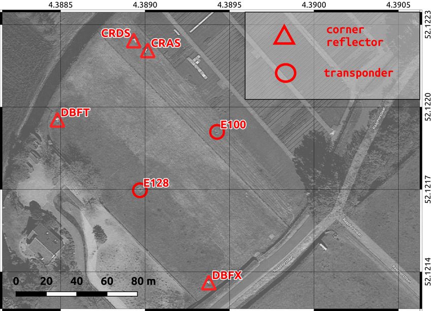
CZIKHARDT ET AL., JUN 2021, SUBMITTED TO IEEE TRANSACTIONS ON GEOSCIENCE AND REMOTE SENSING                                                         3

                             TABLE II                                                                        TABLE III
 S ENTINEL -1 ACQUISITION TIMES SCHEDULED FOR TRANSPONDERS 141                   S ENTINEL -1 ACQUISITION TIMES SCHEDULED FOR TRANSPONDERS 100
    AND 148 AT THE JABO TEST SITE . T HE SUFFIX BEHIND THE TRACK                   AND 128 AT THE WASS TEST SITE . T HE SUFFIX BEHIND THE TRACK
     NUMBER INDICATES THE ASCENDING AND DESCENDING ORBIT                            NUMBER INDICATES THE ASCENDING AND DESCENDING ORBIT
                          DIRECTION .                                                                    DIRECTION .

                                        incidence          zero-Doppler                                          incidence         zero-Doppler
 Track               UTC                                                         Track           UTC
                                        angle              direction                                             angle             direction

 124d                05:02              37.14◦             100.32◦               110d            05:58           36.69◦            100.54◦
 051d                04:54              45.60◦             98.79◦                037d            05:50           44.65◦            98.92◦
 073a                16:43              41.78◦             260.48◦               161a            17:33           41.76◦            260.46◦
 175a                16:35              32.48◦             258.93◦               088a            17:25           33.24◦            258.83◦

                                                                                number of Sentinel-1 data used for the operational period
                                                                                of the tested transponders. The effective acquisition interval
                                                                                for the two Sentinel-1 satellites is 6-days. Due to the chosen
                                                                                settings of the transponders only data in VV polarisation is
                                                                                used for the analysis.
                                                                                   SAR time series analysis of the transponders is performed
                                                                                using the open-source toolbox GECORIS [11]. For the
                                                                                position of each transponder in each of the SLCs, an image
                                                                                patch of 10×10 resolution cells is selected and oversampled by
                                                                                a factor 32 in the frequency domain by zero-padding. Then, we
                                                                                estimate the precise peak position and amplitude by fitting a
                                                                                2D elliptic paraboloid over a small image subpatch, centered at
                                                                                the oversampled amplitude maximum of the initial patch. This
                                                                                procedure guarantees a peak detection precision of better than
                                                                                1/100 pixel [12]–[14], which is equivalent to an uncertainty
Fig. 3. Wassenaar test site, The Netherlands: experiment setup with transpon-   of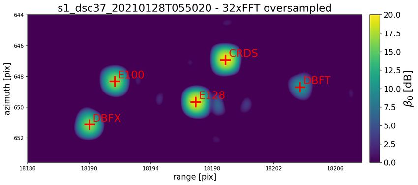
CZIKHARDT ET AL., JUN 2021, SUBMITTED TO IEEE TRANSACTIONS ON GEOSCIENCE AND REMOTE SENSING                                                                  4

                                                             TABLE IV
                        S UMMARY OF THE FOUR TESTED TRANSPONDERS AND S ENTINEL -1 DATA USED UNTIL 28 M ARCH 2021

                                                         Operational                                       No. Sentinel-1A+B acquisitions
 Transponder                   Location
                                                         since                            ascending                        descending

      100          WASS, Wassenaar, Netherlands          2019-06-19                       104 + 105                          107 + 106
      128          WASS, Wassenaar, Netherlands          2020-04-04                       56 + 58                            58 + 58
      141        JABO, Jaslovske Bohunice, Slovakia      2020-07-09                       41 + 42                            41 + 40
      148        JABO, Jaslovske Bohunice, Slovakia      2020-07-09                       41 + 42                            41 + 40

Fig. 4. The radar brightness β0 image patch showing two transponders
(units 141 and 148) at the JABO test site, from ascending track 73 (top row)
and descending track 124 (bottom row) for a single acquisition. Left: Raw
data, and right: oversampled data, factor 32.

of a firmware problem, causing the unit not to switch on
during these satellite overpasses. These outliers were removed
from the time series analysis using the three median absolute                  Fig. 5. RCS time series of transponders 141 and 148 at the JABO test site, for
deviations (MAD) criterion [20].                                               the four Sentinel-1 tracks. The dashed vertical line represents the installation
   Fig. 6 shows an example of the oversampled radar bright-                    time.
ness for all reflectors at the WASS test site.
   The RCS time series statistics for all four transponders are
summarized in Table V. The temporal average RCS of the
units 128, 141, and 148 ranges from 42 dBm2 to 45 dBm2
across Sentinel-1 tracks, while the temporal average RCS of
unit 100, which is an older prototype, is approximately 4 dB
lower. Note that 45 dBm2 is equivalent to a triangular trihedral
corner reflector with a leg-length longer than 2.0 m. These
values are in agreement with the theoretical value computed
using (1).
      a) Alignment sensitivity: Table V shows that the RCS
averages differ between tracks, depending on incidence angle                   Fig. 6. The radar brightness β0 image patch showing all reflectors at the
and zero-Doppler direction, see Tab. II and III, resulting                     WASS test site.
in antenna misalignment and subsequently RCS attenuation.
The misalignment in the elevation (∆θ) is computed as the
acquisition’s incidence angle minus the antenna’s elevation tilt               an equivalent misalignment would yield an attenuation of
(32◦ ) and the misalignment in the azimuth (∆α) is computed                    ∼1.5 dB. Considering a SCR of 20 dB, a 3 dB loss increases
as the acquisition’s zero-Doppler angle minus 90◦ minus the                    the phase error by ∼0.1 mm [19], [21]. We approximate
antenna’s azimuth squint (12◦ ). Fig. 7 shows this average                     the observed attenuation by a quadratic polynomial via a
RCS plotted against a misalignment in elevation and azimuth                    weighted-least-squares (WLS) fit (excluding the data from
angles. We observe maximally 3 dB RCS loss for 13◦ and                         prototype transponder 100 due to its constant offset). The only
−3◦ misalignment in elevation and azimuth angles, respec-                      large residual appears for unit 128, track 37, which may be due
tively. Compared to a triangular trihedral corner reflector,                   to a slightly erroneous antenna orientation within the sealed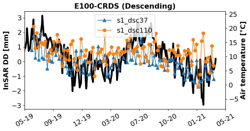
CZIKHARDT ET AL., JUN 2021, SUBMITTED TO IEEE TRANSACTIONS ON GEOSCIENCE AND REMOTE SENSING                                                              5

                                                               TABLE V
                     R ADIOMETRIC STATISTICS OF THE FOUR TRANSPONDERS ON FOUR INDEPENDENT S ENTINEL -1 TIME SERIES .

                        Transponder           No.        Track             Misalignment [deg]         RCS [dBm2 ]      Avg. SCR
                                          acquisitions                    ∆elevation ∆azimuth         mean   std         [dB]
                        100                   107        37d                     4.7       −1.5       37.25  .58           28.65
                                              106        110d                   12.7       −3.1       38.41  .68           29.41
                                              104        161a                    9.8        2.5       37.74  .46           29.24
                                              105        88a                      .2          .8      40.30  .46           33.40
                        128                    58        37d                     4.7       −1.5       40.26  .69           31.66
                                              58         110d                   12.7       −3.1       41.59  .68           32.59
                                              56         161d                    9.8        2.5       42.69  .51           34.19
                                              58         88a                      .2          .8      44.90  .30           38.00
                        141                    41        124d                    5.1       −1.7       42.71  .42           34.55
                                              40         51d                    13.6       −3.2       42.45  .63           37.38
                                              41         73a                     9.8        2.5       45.19  .58           35.20
                                              42         175a                     .5          .9      45.18  .40           39.75
                        148                    37        124d                    5.1       −1.7       42.71  .42           34.55
                                              36         51d                    13.6       −3.2       42.26  .62           36.85
                                              37         73a                     9.8        2.5       42.90  .35           32.46
                                              38         175a                     .5          .9      44.22  .36           36.09

Fig. 7. RCS versus antenna misalignment in elevation (∆θ) and azimuth
(∆α) angles. A weighted-least-squares fit approximates the attenuation by a
quadratic polynomial. Error-bars are 2.5 sigma.

casing of the transponder.
      b) Temporal stability: Comparing the temporal RCS sta-
bility of the transponders with conventional corner reflectors,
see Table VI, we find that despite the higher average RCS
of the transponders, their RCS standard deviations, σRCS , are
significantly higher. For the WASS test site, both the reflectors
and the transponders experience identical clutter conditions,                 Fig. 8. RCS variability versus surface temperature for the four transponders,
                                                                              including Pearson’s sample correlation coefficient r.
which implies that the observed σRCS is not influenced by the
clutter. In fact, the temporal RCS stability of the transponders
is comparable to the DBFT reflector, which has a more than
10 dB lower RCS. In section IV-B we show the implications                     neither do the descending data of the JABO test site. However,
of the RCS stability on the temporal phase stability.                         there is a significant correlation of −0.82 and −0.53 for the
      c) Susceptibility to systematic temporal variations: For a              ascending data of the JABO test site, for units 141 and 148,
correct interpretation of transponder time series, it is important            respectively. This temperature dependency is observed (i) in
to understand whether the RCS is susceptible to systematic                    only one of the two test sites (JABO), (ii) in only one of the
temporal variations. The scatter plots in Fig. 8 show RCS time                two viewing geometries (ascending), (iii) for environmental
series of the transponders plotted againts the hourly surface                 temperatures higher than 20◦ C, which only occur in the
temperatures. The ascending tracks, i.e., the yellow triangles                ascending (afternoon) orbits, and (iv) in two independent units
in Fig. 8, acquired in the afternoon, typically experience a                  (141 and 148). This suggests that temperature variations do not
higher temperature range over the seasons than the descending                 necessarily affect the RCS, but if they do, it occurs mainly for
tracks.                                                                       temperatures higher than 20◦ C. In those cases, an increase in
   The RCS variability of the units in the WASS test site                     temperature results in a (slight) decrease of RCS for these
does not show a significant correlation with temperature, and                 acquisitions. Note that this would lead to a 1 dBm2 reduction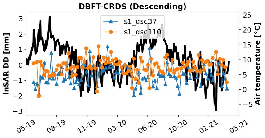
CZIKHARDT ET AL., JUN 2021, SUBMITTED TO IEEE TRANSACTIONS ON GEOSCIENCE AND REMOTE SENSING 6
TABLE VI
RCS STANDARD DEVIATIONS FOR CORNER REFLECTORS AND TRANSPONDERS , IN [ D B M2 ].
σRCS
Target Type Site average RCS
ASC88 ASC161 DSC37 DSC110
CRAS / CRDS reflector WASS 39.0 .13 .19 .14 .19
DBFX reflector WASS 35.4 .24 .21 .16 .22
DBFT reflector WASS 28.6 .44 .42 .47 .44
100 transponder WASS 38.4 .58 .68 .46 .46
128 transponder WASS 42.4 .69 .68 .51 .30
141 transponder JABO 43.9 .42 .63 .58 .40
148 transponder JABO 43.4 .25 .62 .35 .36
in RCS, hence, a 1 dB reduction in SCR, which is equivalent transponder prototypes by [23], with a correlation coefficient
to less than 0.2◦ phase error for an SCR>30. of 0.8.
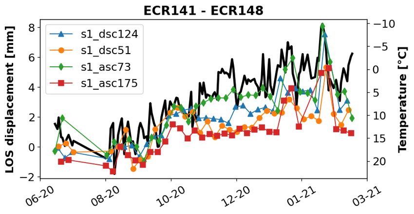
For the transponders at test site JABO, we cannot compute
independent phase DD’s as there is no nearby reference
B. InSAR phase stability corner reflector. Therefore, Fig. 12 only shows phase DD’s,
Deploying compact transponders is arguably most interest- converted to LOS displacements, over the very short baseline
ing for applications that use the phase information, i.e., SAR between units 141 and 148. Assuming the same temperature
interferometry. This requires an assessment of the reliability dependency for both the units, it should cancel out over this
and stability of the transponder phase. At the WASS test baseline. However, a residual correlation of the InSAR phases
site we evaluate this using a configuration that combines with the surface temperature is apparent. Unfortunately, in this
transponders and corner reflectors at distances of less than case we cannot rule out actual subsidence or uplift of one of
70 m, which results in an atmospheric differential signal that the concrete blocks carrying the transponders.
is maximally 0.1 mm in the most extreme situations, but on In Fig. 12 we also compare the LOS displacement time
average 0.03 mm [22], corresponding to 1.3◦ and 0.4◦ for series with the precipitation and snow cover data of test site
C-band, respectively. This allows us to evaluate the temporal JABO. The highest displacement gradient aligns with the time
coherence, i.e. the phase stability, of the transponders, as the of the highest cumulative precipitation, in September 2020.
phase variance should be dominated by the clutter, described The sudden 2 mm phase jumps in January and February of
by the SCR of the transponders, and the sensor’s thermal noise. 2021 are clearly a consequence of the snow and ice cover on
Flattened and topography-corrected interferograms were the transponder’s radomes, as shown by the snow cover time
computed for all Sentinel-1 stacks, and subsequently interfer- series in Fig. 12.
ometric phase time series, evaluated at the IRF peaks, were To compensate for the influence of temperature on phase,
used to compute double-difference phase time series between the transponders would need to have an active temperature
transponders and reflectors. Fig. 9 shows the double-difference control system, such as used by calibration transponders
(DD) phase time series between a transponder and a reference [24]. This would, however, increase the complexity, energy
reflector, both for the ascending and the descending oriented consumption, and consequently the cost of the transponders.
antennas, for all Sentinel-1 tracks. As the seasonal signal is ap- Instead, we find that secular and seasonal effects in the
parent in the time series, we also plot the surface temperature time series can be effectively modelled in the post-processing,
readings of the nearest meteo-station (Voorschoten) obtained as long as they remain trend-stationary. Our results show
at the whole hour closest to the Sentinel-1 acquisition. that rather than using a universal correction, each individual
To verify that this signal is not coming from the reference transponder requires unique modelling. For each track, we esti-
reflectors, we also compute DD time series between the inde- mate and remove the (seasonal) temperature-dependent signal
pendent reference reflectors, see Fig. 10. Since the seasonal from the InSAR DD time series ∆φt for epochs t ∈ (t1 ; tN ),
signal is not visible for this baseline, we can attribute the assuming the functional model
temporal variability in Fig. 9 uniquely to the transponders.
Likewise, scatter plots of the LOS displacement against the ∆φt1 1 Tt1
temperature, see Fig.11, from the ascending tracks, show a
∆φt2 1 T
significant correlation for the transponders, while practically 4π C
t2
E{ . } = − , (3)
. ..
no correlation for CRs. The results from repeated levelling . λ . K
. . . T
measurements between the concrete slabs carrying the reflec-
tors exclude an actual displacement as a potential cause of ∆φtN 1 TtN
the seasonal signal. Therefore, the phase measurements of the
transponders are indeed sensitive to the temperature variations, where C is the constant offset, T the measured temperatures,
with a typical dependency of 0.07–0.15 mm/◦ C. This phase and KT is the temperature-dependent scaling factor. The time-
sensitivity to temperature was also observed for other compact dependent trend (drift) was not parameterized in the (3), as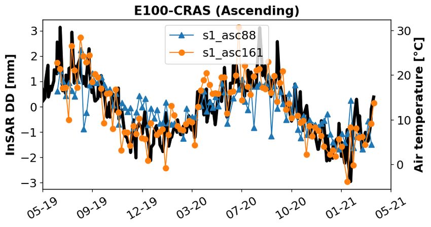
CZIKHARDT ET AL., JUN 2021, SUBMITTED TO IEEE TRANSACTIONS ON GEOSCIENCE AND REMOTE SENSING                                                                   7

Fig. 9. InSAR phase double-difference (DD) for units 100 and 128, relative to a reference corner reflector, plotted against temperature for test site WASS.

Fig. 10. InSAR phase double-differences (DD) for two reference corner reflectors, plotted against air temperature for test site WASS.

Fig. 11. InSAR LOS displacement of transponders (units 100 and 128) and
reflectors (DBFT and DBFX) plotted against temperature, for test site WASS.

no displacement trend is observed from the levelling mea-
surements. However, we estimate the drift from the residuals                   Fig. 12. Time series of InSAR phase double-differences (LOS displacement)
and test its significance using the parameter significance test                between units 141 and 148, and surface temperature, precipitation, and snow
[25]. The estimated drift values are reported in Table VII.                    cover for test site JABO.
For unit 100, in track 88a and 37d, the estimated drifts are
significant (level of significance α = 0.01), while neither of
CZIKHARDT ET AL., JUN 2021, SUBMITTED TO IEEE TRANSACTIONS ON GEOSCIENCE AND REMOTE SENSING                                                   8

                             TABLE VII
I N SAR DOUBLE - DIFFERENCE (DD) PHASE STANDARD DEVIATION (STD)
    AND DRIFT, FOR TRANSPONDERS 100, 128, 141, AND 148, AND FOR
 REFLECTORS CRAS, CRDS, DBFT, AND DBFX. A BBREVIATION DETR .
                       STANDS FOR DETRENDED .

 Baseline       Track   InSAR DD phase STD [mm]       Residual drift
                          predicted     observed         [mm/yr]
                        SCR     NAD   raw     detr.        ±1σ
   100–CRAS     88a      .2      .5    .8      .5      −0.5 ± 0.1
                161a     .2      .4   1.2      .6      −0.3 ± 0.2
       –CRDS    37d      .2      .6    .8      .6      −0.4 ± 0.1
                110d     .2      .6    .7      .6      −0.3 ± 0.1
   128–CRAS     88a      .2      .3    .9      .7      −0.7 ± 0.4
                161a     .2      .5   1.0      .7      −0.6 ± 0.3      Fig. 13. Transponder dimensions and local topocentric offsets for ascend-
       –CRDS    37d      .2      .6    .6      .6      −0.4 ± 0.3      ing/descending antennas’ phase centers (PC), in millimetres.
                110d     .2      .6    .5      .5      −0.6 ± 0.3
 DBFT–CRAS      88a      .4      .4    .5      .5      −0.2 ± 0.1
                                                                       has not changed over the monitored period, the assumption of
                161a     .4      .4    .6      .6      +0.2 ± 0.1
                                                                       temporal ergodicity fails for the time series of the transpon-
       –CRDS    37d      .5      .5    .6      .6       0.0 ± 0.1
                                                                       ders’ peak responses. In other words, the RCS variations are
                110d     .4      .5    .5      .5       0.0 ± 0.1
 DBFX–CRAS      88a      .3      .3    .5      .5       0.0 ± 0.1
                                                                       fully displayed in the phase instability. Therefore, the NAD
                161a     .3      .3    .6      .6       0.0 ± 0.1
                                                                       provides a better STD proxy for the transponders.
      – CRDS    37d      .3      .3    .5      .5      −0.3 ± 0.1
                                                                          Removing the trend and seasonal components lowers the
                110d     .3      .3    .5      .5      −0.1 ± 0.1      STDs, cf. Table VII, where the most notable improvement is
      141–148   73a      .1      .3   1.7      .8      +0.9 ± 0.8      observed for the ascending tracks, which are more affected
                175a     .1      .3   1.3      .9      +1.0 ± 0.9      by temperature variations. For T/R baselines with units 100
                51d      .1      .3   1.9     1.1      +0.9 ± 1.1      and 128, we observe an average STD of 0.6 mm across
                124d     .1      .3   1.6     1.0      +1.1 ± 1.0      all Sentinel-1 tracks. For T/T baseline 141–148, at test site
                                                                       JABO, the phase shifts caused by the temporary snow/ice
                                                                       cover increase the estimated phase STD up to 1.1 mm. The
the estimated drifts of unit 128 could be proven significant.          standard deviations of the undifferenced single epoch phase
Since the estimated residual drifts over the baseline between          measurements of the transponders (σψT in (4)) vary between
the corner reflectors are not significant, see Fig. 10, we reject      0.3 and 0.8 mm.
the hypothesis that reference reflectors have an influence on the
observed drift of the transponders. Longer time series would           C. Absolute Positioning
be needed to obtain a more reliable estimate of the phase drift.
                                                                          The positions of the transponder’s antenna phase centres
Nonetheless, we can safely state that it is smaller than 1 mm
                                                                       (both ascending and descending) in a Terrestrial Reference
per year.
                                                                       Frame (TRF) were determined applying a two-step procedure.
   After removing the estimated temperature-dependent signal
                                                                       First, we determined the coordinates of the transponder ref-
and the residual drift, we assume that the phase residuals
                                                                       erence point, i.e., the northwestern corner of the base-plate,
are representative of the phase noise and compute the stan-
                                                                       see Fig. 13, using GNSS. For the JABO test site, we used
dard deviation (STD) of the residuals. Table VII shows the
                                                                       static GNSS observations for one hour (with a geodetic-grade
estimated STDs for the transponder-reflector (T/R), reflector-
                                                                       receiver Trimble R10), connected to the ETRS89 coordinate
reflector (R/R), and transponder-transponder (T/T) baselines
                                                                       reference system (ETRF2000 reference frame) via the nearby
before (‘raw’) and after the trend removal (‘detrended’). We
                                                                       permanent reference station JABO (SKPOS network). For
compare the estimated STD with the STD predicted using the
                                                                       the WASS test site, we used four 90-seconds GNSS RTK
normalized amplitude dispersion (NAD) [26] and the temporal
                                                                       observations (with a geodetic-grade receiver Trimble R8), con-
average SCR [21]. For the reflectors CRAS and CRDS, we
                                                                       nected to the ETRS89 coordinate reference system (ETRF2000
have a reliable estimate of their long-term phase STD. Their
                                                                       reference frame) using the NETPOS processing service of
undifferenced single epoch phase STD is σψCR = 0.11 mm
                                                                       the Dutch Kadaster. Second, we computed the phase centre
[19]. Therefore, an estimate of the double-difference phase
                                                                       coordinates, for each of the antennas, from the reference point
STD for a T/R baseline is obtained by error propagation
                                                                       coordinates using local coordinate offsets supplied by the
(assuming uncorrelated measurements) as:
                                                                       manufacturer, see Fig. 13.
                  σ∆φT/R = (2σψ2 R + 2σψ2 T )1/2                 (4)      The accuracy (repeatability) of the TRF coordinates is 1–
                                                                       2 cm in the horizontal and 3 cm in the vertical direction.
where σψT is computed either from NAD or SCR. Table VII                Orbit state vectors of Sentinel-1 satellites are given in the
shows that the SCR-based estimation of the phase STD gives             ITRF2014 reference frame with a sampling rate of 10 seconds,
overly optimistic values. As the clutter of the transponders           determined by the on-board GNSS receiver.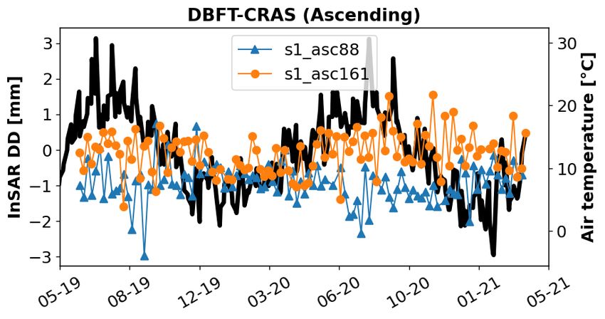
CZIKHARDT ET AL., JUN 2021, SUBMITTED TO IEEE TRANSACTIONS ON GEOSCIENCE AND REMOTE SENSING                                                   9

   Absolute Positioning Errors (APE) are epoch-wise differ-
ences between the detected subpixel peak coordinates and
the expected radar coordinates computed from the precise
TRF positions via the inverse range-Doppler equations [27],
correcting for all SAR timing biases. The APE in range (rg)
and azimuth (az) is computed as:
          APErg = (τpeak, IPF − τpredicted ) · c
                                                                (5)
          APEaz = (tpeak, IPF − tpredicted ) · vzeroDoppler ,
where vzeroDoppler is the satellite’s ground-track zero-Doppler
velocity. τpeak, IPF and tpeak, IPF are the azimuth and range time,
respectively, of the sub-pixel peak positions in the SLC images
as processed by the Sentinel-1’s instrument processing facility
(IPF). Predicted timings, τpredicted and tpredicted , are composed
of individual timing biases, i.e.,
  τpredicted = τITRF + ∆τSET + ∆τtropo + ∆τiono + ∆τDoppler ,
  tpredicted = tITRF + ∆tSET + ∆tbistatic + ∆tFM-rate ,
                                                                (6)   Fig. 14. Absolute Positioning Errors (APE) of transponder 141 from ascend-
                                                                      ing track.
where:
   • ITRF represents positions directly obtained solving the
      range-Doppler equations from GNSS-determined coordi-            [31]. According to the cross-validation of the independently
      nates in ITRS (ITRF2014 reference frame) at the particu-        generated orbit solutions by [31], an orbit accuracy of ∼3 cm
      lar acquisition epoch. The initial coordinates in ETRS89        can be assumed. Considering the limited spatio-temporal res-
      (ETRF2000 reference frame) are first transformed to             olution of the ERA5 model used for troposheric delay cor-
      ITRS at the particular acquisition epoch, hence reflecting      rection, and considering the RMS values of the TEC maps of
      the plate motion.                                               CODE ionospheric models, both tropospheric and ionospheric
   • SET represents timing corrections computed from                  delay corrections could be assumed to exhibit an accuracy of
      topocentric solid earth tides displacements, hence trans-       ∼10 cm [22].
      forming from a ‘tide free’ position (ITRF) to the instan-          Using simple error propagation, these effects contribute to
      taneous position as seen by the satellite (adding a per-        an overall prediction uncertainty (repeatability) of ∼11 cm in
      manent “mean tide”, as well as a periodic components of         range and ∼4 cm in azimuth. The average SCR of reflectors
      tidal displacement using IERS SET displacement models           CRAS and CRDS, varies between 28–32 dB, yields a CRB of
      [8]).                                                           28 cm and 4 cm in the azimuth and range directions, respec-
   • tropo is the range timing correction for the slant tropo-        tively. For these CRs, we achieve an average STD of 42 cm
      spheric signal delay (modelled using the ECMWF ERA5             and 13 cm in the azimuth and range directions, respectively.
      model [28]).                                                    For Sentinel-1 IW products, [14] reports an achievable STD
   • iono is the range timing correction for the slant iono-          limit of 49.2 cm and 8.3 cm for azimuth and range, respec-
      spheric signal delay (modelled using the CODE IGS               tively, given 1.5 m triangular trihedral reflectors. Therefore,
      global ionospheric model [29]).                                 we consider our APE computation framework sufficient for
   • bistatic is the residual bistatic correction of the Sentinel-1   precise APE analysis of the transponders.
      IPF in the azimuth timing [14].                                    Here, the absolute SAR positioning accuracy of the
   • Doppler are Doppler-centroid-induced range timing cor-           transponders is evaluated. In Table VIII, average observed
      rections [14], and                                              APE and its temporal standard deviation (STD) are reported.
   • FM represents the FM-rate mismatch of Sentinel-1 IPF                Fig. 16 shows histograms of APE time series for the
      in the azimuth timing [14].                                     tested transponders. Observed systematic differences in the
Fig. 14 shows these corrections for transponder 141. Individual       range coordinate are primarily caused by the internal elec-
points in the figure represent epoch-wise SLC measurements.           tronic delay of the transponders. An approximate internal
To verify the accuracy of the established APE computation             electronic delay of ∼1.5 m (10−9 s), including the antennas
framework, we compute APE time series for the four reference          and protective radome, was estimated by [5]. However, the
reflectors at test site WASS, see Fig. 15. The observed APE           observed average range differences vary between −1.24 m
and its temporal variance are limited by the Cramer-Rao               to −2.10 m. Moreover, different internal delays are observed
Lower Bound (CRB) of the peak variance, determined by the             across the individual transponders and between ascending and
reflector’s SCR and the azimuth/range SLC resolutions [30].           descending tracks, see Fig. 17. Fig. 18 shows average range
The accuracy of the GNSS-determined TRF coordinates is 1–             delays plotted against the antenna misalignment in elevation
2 cm in the horizontal and 3 cm in the vertical direction.            and azimuth angles. We observe nonsystematic shifts between
The Sentinel-1 orbital state-vectors have a 3D RMS of 5 cm            individual transponders. We also observe an apparent shift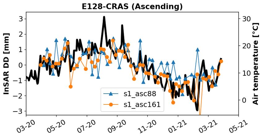
CZIKHARDT ET AL., JUN 2021, SUBMITTED TO IEEE TRANSACTIONS ON GEOSCIENCE AND REMOTE SENSING                                                  10

Fig. 15. Absolute Positioning Errors (APE) of the reference corner reflectors at test site WASS.

                            TABLE VIII                                         coordinate differences are all within the confidence interval of
A BSOLUTE P OSITIONING E RRORS (APE) OF THE TESTED TRANSPONDERS                their standard deviations. For azimuth standard deviations, we
                    ON S ENTINEL -1 TIME SERIES .
                                                                               reach the limit dictated by the SCR (CRB) and the azimuth
 Transponder     Track                    APE ±1σ [cm]
                                                                               resolution (∼22 m). More optimistic values are likely the result
                                azimuth                    range
                                                                               of the biased SCR estimate, see Sec. IV-A.
          100    88a          14.0   ±    36.6        −144.3   ±   13.5
                 161a         24.2   ±    32.7        −136.5   ±   14.1                       V. D ISCUSSION AND C ONCLUSIONS
                 37d         −57.8   ±    39.7        −133.3   ±   12.5           From the experimental results with four compact transpon-
                 110d         −2.0   ±    39.1        −140.9   ±   13.9        ders manufactured by [5], installed at two different test sites,
          128    88a          16.4   ±    35.2        −164.7   ±   16.8        we conclude that they have an average RCS of 40-45 dBm2 ,
                 161a         28.8   ±    27.9        −161.2   ±   16.9        which is comparable to a triangular trihedral corner reflector
                 37d          −3.5   ±    26.5        −210.4   ±   16.1        with a leg length of 2.0 m.
                 110d          6.7   ±    33.3        −208.7   ±   18.8           An antenna misalignment by 12 and 3 degrees in ele-
          141    88a          19.2   ±    26.3        −123.6   ±   15.8        vation and azimuth angles, respectively (extreme values for
                 161a         −0.6   ±    33.7        −125.3   ±   19.0        Sentinel-1 over European latitudes), yields an RCS attenuation
                 37d         −23.7   ±    25.7        −188.0   ±   14.0        of up to 3 dB. While this attenuation is rather modest, by
                 110d          5.6   ±    30.1        −183.8   ±   17.2        modifying the default antenna alignment for the site-specific
          148    88a          16.1   ±    20.8        −145.2   ±   17.3        viewing geometry this attenuation can be further reduced.
                 161a         29.7   ±    37.0        −137.2   ±   17.9        The temporal standard deviation of the transponders’ RCS
                 37d          20.3   ±    24.1        −151.2   ±   12.6        is up to 0.7 dB, which is more than two times the standard
                 110d          8.5   ±    38.4        −151.9   ±   12.2        deviation observed for a corner reflector of equivalent RCS,
                                                                               considering the 0.25 dB radiometric stability of the Sentinel-1
                                                                               SLC measurements [32]. For some transponder units, and for
between ascending (negative ∆α) and descending (positive                       sites with temperatures exceeding 20 ◦ C, the RCS variability
∆α) tracks, which is highest for transponder 141 (>0.5 m) and                  is correlated with temperature variations. We observed this
smallest for transponder 148 (
CZIKHARDT ET AL., JUN 2021, SUBMITTED TO IEEE TRANSACTIONS ON GEOSCIENCE AND REMOTE SENSING 11 Fig. 16. Absolute Positioning Errors (APE) of the transponders from Sentinel-1 tracks be proven to be dependent on incidence angle or the azimuth with environmental temperature variations, showing variations of the zero-Doppler plane. Thus, for absolute centimeter- within a range of 6 mm. These can be modelled using a level geodetic positioning purposes, the transponders would simple scaling factor, that needs to be computed specific per require individual calibration models, similar as applied for transponder unit. geodetic GNSS antennas. The variable part of the absolute Estimating this temperature-dependent scaling factor, i.e., SAR positioning, in azimuth and range, is found to have a removing the seasonal variability, yields an observed InSAR precision of 39.1 cm and 16.2 cm, respectively. phase standard deviation of 0.5–0.7 mm in the LOS direction. Regarding the precision of the double-difference interfer- Regarding a potential phase drift, giving the maximum time ometric phase, relative to a passive reference reflector, we interval of 21 months analyzed in this study, we find that observe a phase standard deviation varying between 0.5 and if apparent at all, it is less than 1 mm/y. This is especially 1.2 mm, which implies a single-epoch undifferenced standard important for long-term InSAR reliability. deviation of the transponder phase of 0.3 to 0.8 mm. Finally, snow or ice cover on the transponder radome may Yet, we observe the phase to be significantly correlated cause undesired phase spikes with larger magnitudes than the
CZIKHARDT ET AL., JUN 2021, SUBMITTED TO IEEE TRANSACTIONS ON GEOSCIENCE AND REMOTE SENSING                                                              12

                                                                               for the specific satellite orbits of interest. For example, for
                                                                               applications that require more (or less) sensitivity to vertical
                                                                               or horizontal displacement components, this is a parameter
                                                                               that can be optimized. Third, the transponders ideally need
                                                                               to include a calibration report with specific information on
                                                                               the constant and temperature-dependent internal delays. Al-
                                                                               ternatively, an on-site calibration campaign may be required,
                                                                               where we recommend to compute baselines with permanently
                                                                               installed corner reflectors of sufficient size and with a well-
                                                                               known temporal behavior. Calibration activities containing
                                                                               two transponder units may not be sensitive to correlated
                                                                               signals, such as temperature variability. The duration of the
                                                                               calibration depends on the specific application. Several cross-
                                                                               track acquisitions are already sufficient to obtain a reasonable
                                                                               estimate of the RCS and the internal delay.
                                                                                  For further research, we recommend extending experiments
                                                                               using longer Sentinel-1 and Radarsat-2 SAR time series to
                                                                               further improve robust estimates on the InSAR phase stability,
                                                                               especially on the possible secular drift.
                                                                                  Finally, we strongly support international activities in per-
                                                                               manent deployment of transponders, mechanically coupled to
                                                                               GNSS antenna infrastructure and to tide gauges.
Fig. 17. Absolute Positioning Errors (APE) of the corner reflectors
(CRAS/CRDS) and the transponders 100/128 at the WASS test site, using                                       R EFERENCES
Sentinel-1 data.
                                                                                [1] T. Gruber, J. Ågren, D. Angermann, A. Ellmann, A. Engfeldt,
                                                                                    C. Gisinger, L. Jaworski, S. Marila, J. Nastula, F. Nilfouroushan,
                                                                                    X. Oikonomidou, M. Poutanen, T. Saari, M. Schlaak, A. Światek,
                                                                                    S. Varbla, and R. Zdunek, “Geodetic SAR for Height System Unification
                                                                                    and Sea Level Research—Observation Concept and Preliminary Results
                                                                                    in the Baltic Sea,” Remote Sens., vol. 12, no. 22, 2020.
                                                                                [2] C. Gisinger, M. Eineder, R. Brcic, U. Balss, T. Gruber, X. Oikonomidou,
                                                                                    and M. Heinze, “First Experiences with Active C-Band Radar Reflectors
                                                                                    and Sentinel-1,” in IGARSS 2020 - 2020 IEEE International Geoscience
                                                                                    and Remote Sensing Symposium, 2020, pp. 1165–1168.
                                                                                [3] P. Mahapatra, S. Samiei-Esfahany, H. van der Marel, and R. Hanssen,
                                                                                    “On the Use of Transponders as Coherent Radar Targets for SAR
                                                                                    Interferometry,” IEEE Trans. Geosci. Remote Sens., vol. 52, no. 3, pp.
Fig. 18. Internal range delay versus antennas misalignment in elevation (∆θ)        1869–1878, March 2014.
and azimuth (∆α) angles. Error-bars are 2.5 sigma.                              [4] P. Mahapatra, H. van der Marel, F. van Leijen, S. Samiei Esfahany,
                                                                                    R. Klees, and R. Hanssen, “InSAR datum connection using GNSS-
                                                                                    augmented radar transponders,” J. Geodesy, Jun. 2017.
                                                                                [5] Metasensing, “Metasensing bv: Radar solutions - electronic corner
phase accuracy.                                                                     reflector - c band (ecr-c),” https://www.geomatics.metasensing.com/ecr-
  In general, based on our analysis of amplitude and phase,                         c, 2021.
                                                                                [6] D. R. Brunfeldt and F. T. Ulaby, “Active Reflector for Radar Calibra-
we observe that transponder unit cannot be regarded as being                        tion,” IEEE Trans. Geosci. Remote Sens., vol. GE-22, no. 2, pp. 165–169,
equal. In fact different units are specific in terms of their                       1984.
radiometric, geometric, and phase stability. This supports the                  [7] A. Freeman, Y. Shen, and C. L. Werner, “Polarimetric SAR calibration
                                                                                    experiment using active radar calibrators,” IEEE Trans. Geosci. Remote
suggestion of performing unit-specific calibrations, both by the                    Sens., vol. 28, no. 2, pp. 224–240, 1990.
manufacturer and considering site-specific conditions.                          [8] IERS, “International earth rotation and reference systems service,”
                                                                                    https://www.iers.org/, 2021.
                                                                                [9] GKU Slovakia, “Geodetic and Cartographic Institute in Bratislava,
             VI. P RACTICAL R ECOMMENDATIONS                                        Slovakia,” https://www.geoportal.sk/sk/udaje/ortofotomozaika/, 2021.
                                                                               [10] R. Hanssen, “A radar retroreflector device and a method
   The decision whether to deploy transponders is very depen-                       of preparing a radar retroreflector device,” Jun. 21 2017,
dent on the specific case study. Yet, there are a few general                       international Patent WO2018236215A1. [Online]. Available:
considerations that can be recommended for each application.                        https://patents.google.com/patent/WO2018236215A1/en
                                                                               [11] R. Czikhardt, H. van der Marel, and J. Papco, “GECORIS: An Open-
First, estimating the clutter at the location of preferred de-                      Source Toolbox for Analyzing Time Series of Corner Reflectors in
ployment is strongly recommended. The clutter power should                          InSAR Geodesy,” Remote Sens., vol. 13, no. 5, 2021.
be preferably less than 4 dB, to obtain valuable estimates of                  [12] U. Balss et al., “Survey Protocol for Geometric SAR Sensor Analysis,”
                                                                                    German Aerospace Center (DLR), Technical University of Munich
phase, e.g., with a standard deviation of better than 2 mm, and                     (TUM), Remote Sensing Laboratories - University of Zurich (RSL),
a distinct amplitude response. Second, when transponder units                       Tech. Rep., Apr. 2018.
are ordered, the antenna orientation needs to be optimized for                 [13] U. Balss, C. Gisinger, and M. Eineder, “Measurements on the
                                                                                    absolute 2-D and 3-D localization accuracy of TerraSAR-X,”
the specific geographic location of deployment. Note that this                      Remote Sens., vol. 10, no. 4, p. 656, 2018. [Online]. Available:
is not only latitude dependent, but it can also be optimized                        https://doi.org/10.3390/rs10040656
CZIKHARDT ET AL., JUN 2021, SUBMITTED TO IEEE TRANSACTIONS ON GEOSCIENCE AND REMOTE SENSING 13
[14] C. Gisinger, A. Schubert, H. Breit, M. Garthwaite, U. Balss, M. Will- Richard Czikhardt received the M.Sc. degree in
berg, D. Small, M. Eineder, and N. Miranda, “In-Depth Verification of geodesy and cartography in 2017 and is currently
Sentinel-1 and TerraSAR-X Geolocation Accuracy Using the Australian pursuing a Ph.D. degree with the Department of
Corner Reflector Array,” IEEE Trans. Geosci. Remote Sens., vol. 59, Theoretical Geodesy and Geoinformatics, Slovak
no. 2, pp. 1154–1181, Feb. 2021. University of Technology, Bratislava, Slovakia. His
[15] A. Gray, P. Vachon, C. Livingstone, and T. Lukowski, “Synthetic aper- primary research is on Interferometric Synthetic
ture radar calibration using reference reflectors,” IEEE Trans. Geosci. Aperture Radar (InSAR) geodesy, focusing on ad-
Remote Sens., vol. 28, no. 3, pp. 374–383, Mar. 1990. vanced InSAR processing techniques, quality con-
[16] A. Freeman, “SAR calibration: An overview,” IEEE Trans. Geosci. trol, and geodetic integration using artificial radar
Remote Sens., vol. 30, no. 6, pp. 1107–1121, Jun. 1992. reflectors. In 2019, he served as a research intern at
[17] N. Miranda and P. J. Meadows, “Radiometric Calibration of S-1 Level-1 the Department of Geoscience and Remote Sensing,
Products Generated by the S-1 IPF,” European Space Agency (ESA), Delft University of Technology. He has practical experience with InSAR
Tech. Rep., May 2015. software development, time series analysis, image processing, satellite and
[18] R. Piantanida, N. Miranda, and G. Hajduch, “Thermal Denoising of ground-based geodetic techniques and geographic information systems.
Products Generated by the S-1 IPF,” MPC-S1, Tech. Rep., Nov. 2017.
[19] R. Czikhardt, H. van der Marel, F. J. van Leijen, and R. F. Hanssen,
“Estimating signal-to-clutter ratio of InSAR corner reflectors from SAR
time series,” IEEE Geosci. Remote Sens. Lett., vol. PP(99), 2021.
[20] C. Leys, C. Ley, O. Klein, P. Bernard, and L. Licata, “Detecting outliers:
Do not use standard deviation around the mean, use absolute deviation
around the median,” J. Exp. Soc. Psychol., vol. 49, no. 4, pp. 764 – 766, Hans van der Marel received the M.Sc. degree in
2013. geodetic engineering and the Ph.D. (cum laude) de-
[21] P. Dheenathayalan, M. C. Cuenca, P. Hoogeboom, and R. F. Hanssen, gree from the Delft University of Technology, Delft,
“Small reflectors for ground motion monitoring with InSAR,” IEEE The Netherlands, in 1983 and 1988, respectively. He
Trans. Geosci. Remote Sens., vol. 55, no. 12, pp. 6703–6712, Dec. 2017. is an Assistant Professor with the Department of
[22] R. F. Hanssen, Radar interferometry: data interpretation and error Geoscience and Remote Sensing, Delft University of
analysis. Springer, 2001, vol. 2. Technology, Delft, The Netherlands. From Septem-
[23] G. Luzi, P. F. Espı́n-López, F. Mira Pérez, O. Monserrat, and ber 1983 until July 1987, he was a Research Fellow
M. Crosetto, “A Low-Cost Active Reflector for Interferometric Moni- with the Netherlands Organisation for Scientific Re-
toring Based on Sentinel-1 SAR Images,” Sensors, vol. 21, no. 6, 2021. search and worked on the scientific data reduction
[24] S. Raab, B. J. Doering, D. Rudolf, J. Reimann, and M. Schwerdt, for the astronomical satellite Hipparcos. From 1987
“Analysis of an improved temperature management concept for SAR until 1989, he was a Research Fellow with the Netherlands Academy of
system calibration transponders,” in Proceedings of EUSAR 2016: 11th Sciences. In 1989, he became an Assistant Professor with the Delft University
European Conference on Synthetic Aperture Radar, 2016, pp. 1–6. of Technology in Global Navigation Satellite Systems (GNSS), with a specific
[25] K.-R. Koch, Parameter Estimation and Hypothesis Testing in Linear interest in high-precision scientific and meteorological applications of GNSS.
Models, 2nd ed. New York: Springer-Verlag, 1999.
[26] A. Ferretti, C. Prati, and F. Rocca, “Permanent Scatterers in SAR
Interferometry,” IEEE Trans. Geosci. Remote Sens., vol. 39, no. 1, pp.
8–20, Jan. 2001.
[27] I. G. Cumming and F. H. Wong, Digital processing of Synthetic Aperture
Radar data: : Algorithms and Implementation, ser. 1. The address:
Artech House, 1 2005, vol. 1.
Juraj Papco received the Ph.D. degree in geodesy
[28] H. Hersbach and D. Dee, “Era5 reanalysis is in
and cartography from Slovak University of Tech-
production, ecmwf newsletter 147,” pp. 5–6, 2016. [On-
nology, Bratislava, Slovakia, in 2010. Since 2004,
line]. Available: https://www.ecmwf.int/en/newsletter/147/news/era5-
he has been a Researcher and Lecturer in global
reanalysis-production
geodesy and remote sensing with the Slovak Univer-
[29] IGS, “International gnss service,” http://www.igs.org/, 2021.
sity of Technology. As the principal investigator, he
[30] R. Bamler and M. Eineder, “Accuracy of differential shift estimation by
has experience in managing several satellite-InSAR-
correlation and split-bandwidth interferometry for wideband and delta-
related projects, unique for Slovakia territory. His
k SAR systems,” IEEE Geosci. Remote Sens. Lett., vol. 2, no. 2, pp.
main research interests include satellite geodesy,
151–155, Feb. 2005.
GNSS, remote sensing, SAR and InSAR, deforma-
[31] H. Peter, A. Jäggi, J. Fernández, D. Escobar, F. Ayuga, D. Arnold,
tion monitoring, gravity field modelling, gravimetry
M. Wermuth, S. Hackel, M. Otten, W. Simons, P. Visser, U. Hugentobler,
and land surveying.
and P. Féménias, “Sentinel-1A – First precise orbit determination
results,” Advances in Space Research, vol. 60, no. 5, pp. 879 – 892,
2017.
[32] CLS, “Sentinel-1A N-Cyclic Performance Report - 2020-07,” Collecte
Localisation Satellites (CLS), Ramonville Saint-Agne, France, Tech.
Rep., Jul. 2020.
Ramon F. Hanssen (M’04–SM’15) received the
M.Sc. degree in geodetic engineering and the Ph.D.
(cum laude) degree in geodetic engineering from
Delft University of Technology, Delft, The Nether-
lands, in 1993 and 2001, respectively. He was
with the International Institute for Aerospace Survey
and Earth Science, Stuttgart University, the Ger-
man Aerospace Center (DLR), Stanford University
(Fulbright Fellow), and the Scripps Institution of
Oceanography where he worked on microwave re-
mote sensing, radar interferometry, signal process-
ing, and geophysical application development. Since 2008, he has been Antoni
van Leeuwenhoek Professor in geodesy and satellite earth observation at
Delft University of Technology. He is the author of a textbook on radar
interferometry.You can also read