Rstoolbox - a Python library for large-scale analysis of computational protein design data and structural bioinformatics - BMC Bioinformatics
←
→
Page content transcription
If your browser does not render page correctly, please read the page content below
Bonet et al. BMC Bioinformatics    (2019) 20:240
https://doi.org/10.1186/s12859-019-2796-3

 SOFTWARE                                                                                                                                        Open Access

rstoolbox - a Python library for large-scale
analysis of computational protein design
data and structural bioinformatics
Jaume Bonet1,2, Zander Harteveld1,2, Fabian Sesterhenn1,2, Andreas Scheck1,2 and Bruno E. Correia1,2*

  Abstract
  Background: Large-scale datasets of protein structures and sequences are becoming ubiquitous in many domains of
  biological research. Experimental approaches and computational modelling methods are generating biological data at
  an unprecedented rate. The detailed analysis of structure-sequence relationships is critical to unveil governing
  principles of protein folding, stability and function. Computational protein design (CPD) has emerged as an important
  structure-based approach to engineer proteins for novel functions. Generally, CPD workflows rely on the generation of
  large numbers of structural models to search for the optimal structure-sequence configurations. As such, an important
  step of the CPD process is the selection of a small subset of sequences to be experimentally characterized. Given the
  limitations of current CPD scoring functions, multi-step design protocols and elaborated analysis of the decoy
  populations have become essential for the selection of sequences for experimental characterization and the
  success of CPD strategies.
  Results: Here, we present the rstoolbox, a Python library for the analysis of large-scale structural data
  tailored for CPD applications. rstoolbox is oriented towards both CPD software users and developers, being
  easily integrated in analysis workflows. For users, it offers the ability to profile and select decoy sets, which
  may guide multi-step design protocols or for follow-up experimental characterization. rstoolbox provides
  intuitive solutions for the visualization of large sequence/structure datasets (e.g. logo plots and heatmaps) and
  facilitates the analysis of experimental data obtained through traditional biochemical techniques (e.g. circular
  dichroism and surface plasmon resonance) and high-throughput sequencing. For CPD software developers, it
  provides a framework to easily benchmark and compare different CPD approaches. Here, we showcase the
  rstoolbox in both types of applications.
  Conclusions: rstoolbox is a library for the evaluation of protein structures datasets tailored for CPD data. It
  provides interactive access through seamless integration with IPython, while still being suitable for high-
  performance computing. In addition to its functionalities for data analysis and graphical representation, the
  inclusion of rstoolbox in protein design pipelines will allow to easily standardize the selection of design
  candidates, as well as, to improve the overall reproducibility and robustness of CPD selection processes.
  Keywords: rstoolbox, Computational protein design, Protein structural metrics, Scoring, Data analysis

* Correspondence: bruno.correia@epfl.ch
1
 Institute of Bioengineering, École Polytechnique Fédérale de Lausanne,
CH-1015 Lausanne, Switzerland
2
 Swiss Institute of Bioinformatics (SIB), CH-1015 Lausanne, Switzerland

                                        © The Author(s). 2019 Open Access This article is distributed under the terms of the Creative Commons Attribution 4.0
                                        International License (http://creativecommons.org/licenses/by/4.0/), which permits unrestricted use, distribution, and
                                        reproduction in any medium, provided you give appropriate credit to the original author(s) and the source, provide a link to
                                        the Creative Commons license, and indicate if changes were made. The Creative Commons Public Domain Dedication waiver
                                        (http://creativecommons.org/publicdomain/zero/1.0/) applies to the data made available in this article, unless otherwise stated.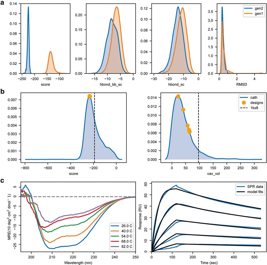
Bonet et al. BMC Bioinformatics   (2019) 20:240                                                                    Page 2 of 13

Background                                                     depending on the number of residues for which se-
The fast-increasing amounts of biomolecular structural         quence design will be performed. Due to the large decoy
data are enabling an unprecedented level of analysis to un-    sets generated in the search for the best design solution,
veil the principles that govern structure-function relation-   as well as the specificities of each design case, re-
ships in biological macromolecules. This wealth of             searchers tend to either generate one-time-use scripts or
structural data has catalysed the development of computa-      analysis scripts provided by third parties [16]. In the first
tional protein design (CPD) methods, which has become a        case, these solutions are not standardized and its logic
popular tool for the structure-based design of proteins        can be difficult to follow. In the second case, these
with novel functions and optimized properties [1]. Due to      scripts can be updated over time without proper
the extremely large size of the sequence-structure space       back-compatibility control. As such, generalized tools to
[2], CPD is an NP-hard problem [3]. Two different ap-          facilitate the management and analysis of the generated
proaches have been tried to address this problem: deter-       data are essential to CPD pipelines.
ministic and heuristic algorithms.                               Here, we present rstoolbox, a Python library to man-
  Deterministic algorithms are aimed towards the search        age and analyse designed decoy sets. The library presents a
of a single-best solution. The OSPREY design suite,            variety of functions to produce multi-parameter scoring
which combines Dead-End Elimination theorems com-              schemes and compare the performance of different CPD
bined with A* search (DEE/A*) [4], is one of the most          protocols. The library can be accessed by users within three
used software relying on this approach. By definition, de-     levels of expertise: a collection of executables for designers
terministic algorithms provide a sorted, continuous list       with limited coding experience, interactive interfaces such
of results. This means that, according to their energy         as Ipython [17] for designers with basic experience in data
function, one will find the best possible solution for a       analysis (i.e. pandas [18]), and a full-fledge API to be used
design problem. Nevertheless, as energy functions are          by developers to benchmark and optimize new CPD proto-
not perfect, the selection of multiple decoys for experi-      cols. This library was developed for direct processing of Ro-
mental validation is necessary [5, 6]. Despite notable         setta output files, but its general architecture makes it easily
successes [7–9], the time requirements for deterministic       adaptable to other CPD software. The applicability of the
design algorithms when working with large proteins or          tools developed expands beyond the analysis of CPD data
de novo design approaches limits their applicability,          making it suitable for general structural bioinformatics
prompting the need for alternative approaches for CPD.         problems (see extended_example notebook in the code’s re-
  Heuristic algorithms, such as those based on Monte           pository). Thus, we foresee that rstoolbox may provide
Carlo (MC) sampling [10], use stochastic sampling              a number of useful functionalities for the broad structural
methods together with scoring functions to guide the           bioinformatics community.
structure and sequence exploration towards an opti-
mized score. These algorithms have the advantage of            Implementation
sampling the sequence-structure space within more rea-         rstoolbox has been implemented extending from
sonable time spans, however, they do not guarantee that        pandas [18], one of the most established Python libraries
the final solutions reached the global minimum [11].           for high-performance data analysis. The rstoolbox li-
Heuristic CPD workflows address this shortcoming in            brary architecture is composed of 4 functional modules
two ways: I) extensive sampling generating large decoy         (Fig. 1): I) rstoolbox.io - provides read/write func-
sets; II) sophisticated ranking and filtering schemes to       tions for multiple data types, including computational de-
discriminate and identify the best solutions. This general     sign simulations and experimental data, in a variety of
approach is used by the Rosetta modelling suite [12],          formats; II) rstoolbox.analysis - provides functions
one of the most widespread CPD tools.                          for sequence and structural analysis of designed decoys;
  For Rosetta, as with other similar approaches, the           III) rstoolbox.plot – plotting functionalities that in-
amount of sampling necessary scales with the degrees of        clude multiple graphical representations for protein se-
freedom (conformational and sequence) of a particular          quence and structure features, such as logo plots [19],
CPD task. Structure prediction simulations such as ab          Ramachandran distributions [20], sequence heatmaps and
initio or docking may require to generate up to 106 de-        other general plotting functions useful for the analysis of
coys to find acceptable solutions [13, 14]. Similarly, for     CPD data; IV) rstoolbox.utils – helper functions
different design problems the sampling scale has been          for data manipulation and conversion, comparison of de-
estimated. Sequence design using static protein back-          signs with native proteins and the creation of amino acid
bones (fixed backbone design) [15] may reach sufficient        profiles to inform further iterations of the design process.
sampling within hundreds of decoys. Protocols that                Additionally, rstoolbox contains 3 table-like data
allow even limited backbone flexibility, dramatically in-      containers defined in the rstoolbox.components
crease the search space, requiring 104 to 106 decoys,          module (Fig. 1): I) DesignFrame - each row is a designed
Bonet et al. BMC Bioinformatics    (2019) 20:240                                                                                   Page 3 of 13

 Fig. 1 rstoolbox library architecture. The io module contains functions for parsing the input data. The input functions in io generate one of
 the three data containers defined in the components module: DesignFrame for decoy populations, SequenceFrame for per-position
 amino acid frequencies and FragmentFrame for Rosetta’s fragments. The other three modules analysis, utils and plot, provide all the
 functions to manipulate, process and visualize the data stored in the different components

decoy and the columns represent decoy properties, such as,               decoys through different scores and evaluation of sequence
structural and energetic scores, sequence, secondary struc-              and structural features. It can be filled with any tabulated,
ture, residues of interest among others; II) Sequence-                   csv or table-like data file. Any table-formatted data can be
Frame - similar to a position-specific scoring matrix                    readily input, as the generation of parsers and integration
(PSSM), obtained from the DesignFrame can be used for                    into the rstoolbox framework is effortless, provid-
sequence and secondary structure enrichment analysis; III)               ing easy compatibility with other CPD software pack-
FragmentFrame - stores fragment sets, a key element in                   ages, in addition to Rosetta. Currently, rstoolbox
Rosetta’s ab initio folding and loop closure protocols. De-              provides parsers for FASTA files, CLUSTALW [21]
rived from pandas.DataFrame [18], all these objects                      and HMMER [22] outputs, Rosetta’s json and silent
can be casted from and to standard data frames, making                   files (Fig. 1).
them compatible with libraries built for data frame analysis                The components of the library can directly interact
and visualization.                                                       with most of the commonly used Python plotting li-
  The DesignFrame is the most general data structure                     braries such as matplotlib [23] or seaborn [24].
of the library. It allows fast sorting and selection of                  Additional plotting functions, such as logo and
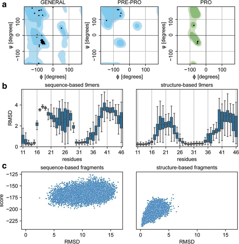
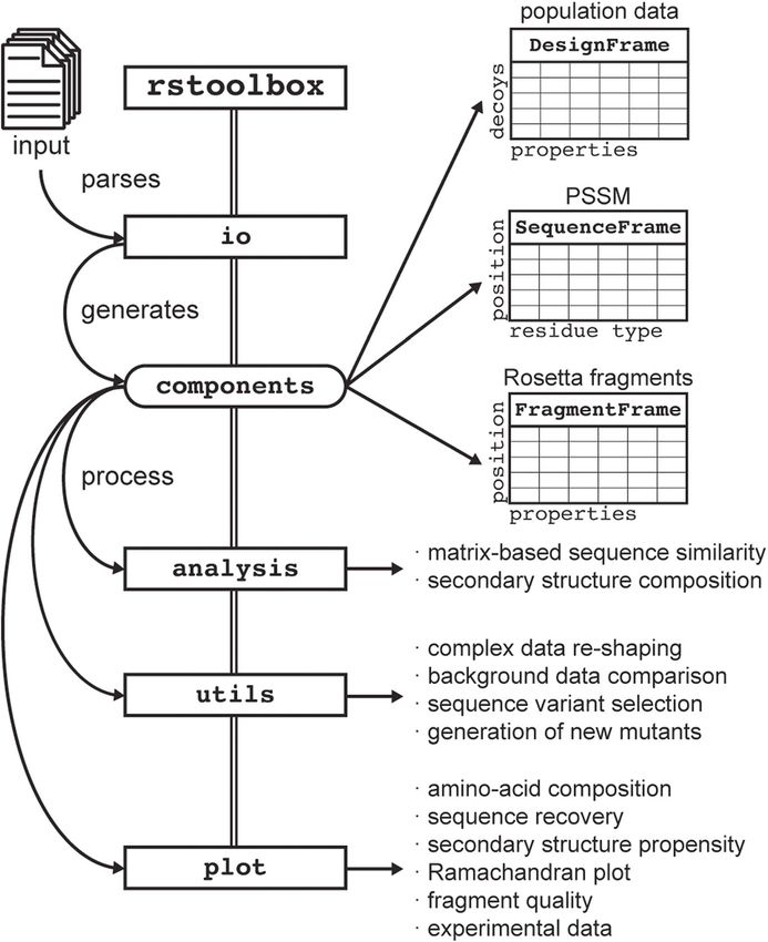
Bonet et al. BMC Bioinformatics       (2019) 20:240                                                                                           Page 4 of 13

Ramachandran plots, are also present to facilitate spe-                         and can be directly installed                      with     PyPI     (pip
cific analysis of CPD data. As mentioned, this library                          install rstoolbox).
has been developed primarily to handle Rosetta out-
puts and thus, rstoolbox accesses Rosetta functions                             Results
to extract structural features from designed decoys (e.                         Analysis of protein backbone features
g. backbone dihedral angles). Nevertheless, many of                             A typical metric to assess the quality of protein back-
the rstoolbox’s functionalities are independent of a                            bone conformations is by comparison of the backbone
local installation of Rosetta. rstoolbox is config-                             dihedral angles with those of the Ramachandran distri-
ured with a continuous integration system to guaran-                            butions [20]. Such evaluation is more relevant in CPD
tee a robust performance upon the addition of new                               strategies that utilize flexible backbone sampling, which
input formats and functionalities. Testing covers more                          have become increasingly used in the field (e.g. loop
than 80% of the library’s code, excluding functions                             modelling [25], de novo design [26]). A culprit often ob-
that have external dependencies from programs like                              served in designs generated using flexible backbone sam-
Rosetta [12], HMMER [22] or CLUSTALW [21]. To                                   pling is that the modelled backbones present dihedral
simplify its general usage, the library has a full API                          angles in disallowed regions of the Ramachandran distri-
documentation with examples of common applications                              butions, meaning that such conformations are likely to

 Fig. 2 Ramachandran plots and fragment quality profiles. Assessment of fragments generated using distinct input data and their effect on Rosetta ab
 initio simulations. With the exception of the panel identifiers, the image was created with the code presented in Table 1. a Ramachandran distribution
 of a query structure. b Fragment quality comparison between sequence- and structure-based fragments. The plot shows a particular region of the
 protein for which sequence-based fragments present much larger structural deviations than structure-based fragments in comparison with the query
 protein. c Rosetta ab initio simulations performed with sequence- (left) or structure-based (right) fragments. Fragments with a better structural mimicry
 relative to the query structure present an improved folding funnel
Bonet et al. BMC Bioinformatics         (2019) 20:240                                                                                            Page 5 of 13

Table 1 Sample code for the evaluation of protein backbone dihedral angles and fragment quality
Action                                             Code Sample
Load                                               import rstoolbox as rs
                                                   import matplotlib.pyplot as plt
                                                   import seaborn as sns
Read                                               # With Rosetta installed, a single structure is scored. The
                                                   # function will return multiple score terms, sequence,
                                                   # secondary structure and phi/psi angles.
                                                   ref = rs.io.get_sequence_and_structure(‘1kx8_d2.pdb’)
                                                   # Loading Rosetta fragments
                                                   seqfrags = rs.io.parse_rosetta_fragments(‘seq.200.9mers’)
                                                   # With Rosetta, structural similarity of the fragments can be measured
                                                   seqfrags = seqfrags.add_quality_measure(None, ‘mota_1kx8_d2.pdb’)
                                                   strfrags = rs.io.parse_rosetta_fragments(‘str.200.9mers’)
                                                   strfrags = strfrags.add_quality_measure(None, ‘mota_1kx8_d2.pdb’)
                                                   # Loading ab initio data
                                                   abseq = rs.io.parse_rosetta_file(‘abinitio_seqfrags.minsilent.gz’)
                                                   abstr = rs.io.parse_rosetta_file(‘abinitio_strfrags.minsilent.gz’)
Plot                                               fig = plt.figure(figsize = (170 / 25.4, 170 / 25.4))
                                                   grid = (3, 6)
                                                   # There are 4 flavours of Ramachandran plots available depending on the
                                                   # targeted residues: GENERAL, GLY, PRE-PRO and PRO.
                                                   ax1 = plt.subplot2grid(grid, (0, 0), colspan = 2)
                                                   # Ramachandran is plotted for a single decoy (selected as parameter 1).
                                                   # As a decoy can contain multiple chains, the chain identifier is an
                                                   # ubiquitous attribute in multiple functions of the library.
                                                   rs.plot.plot_ramachandran_single(ref.iloc[0], ‘A’, ax1)
                                                   ax1 = plt.subplot2grid(grid, (0, 2), fig = fig, colspan = 2)
                                                   rs.plot.plot_ramachandran_single(ref.iloc[0], ‘A’, ax1, ‘PRE-PRO’)
                                                   ax1 = plt.subplot2grid(grid, (0, 4), colspan = 2)
                                                   rs.plot.plot_ramachandran_single(ref.iloc[0], ‘A’, ax1, ‘PRO’)
                                                   # Show RMSD match of fragments to the corresponding sequence for a
                                                   # selected region
                                                   ax1 = plt.subplot2grid(grid, (1, 0), colspan = 3)
                                                   ax2 = plt.subplot2grid(grid, (1, 3), colspan = 3, sharey = ax1)
                                                   rs.plot.plot_fragments(seqfrags.slice_region(21, 56),
                                                                            strfrags.slice_region(21, 56), ax1, ax2)
                                                   rs.utils.add_top_title(ax1, ‘sequence-based 9mers’)
                                                   rs.utils.add_top_title(ax2, ‘structure-based 9mers’)
                                                   # DataFrames can directly work with widely spread plotting functions
                                                   ax1 = plt.subplot2grid(grid, (2, 0), colspan = 3)
                                                   sns.scatterplot(x = “rms”, y = “score”, data = abseq, ax = ax1)
                                                   ax2 = plt.subplot2grid(grid, (2, 3), colspan = 3, sharey = ax1, sharex = ax1)
                                                   sns.scatterplot(x = “rms”, y = “score”, data = abstr, ax = ax2)
                                                   rs.utils.add_top_title(ax1, ‘sequence-based fragments’)
                                                   rs.utils.add_top_title(ax2, ‘structure-based fragments’)
                                                   plt.tight_layout()
                                                   plt.savefig(‘BMC_Fig2.png’, dpi = 300)
The code shows how to combine structural data obtained from a protein structure file with fragment quality evaluated by Rosetta and ab initio simulations. Code
comments are presented in italics while functions from the rstoolbox are highlighted in bold. Styling commands are skipped to facilitate reading, but can be
found in the repository’s notebook.

be unrealistic. To identify these problematic structures,                         criterion to select the best designed sequences is on de
rstoolbox provides functions to analyse the dihedral                              novo design. To assess the ability of novel sequences to
angles of decoy sets and represent them in Ramachan-                              refold to the target structures, the Rosetta ab initio
dran plots (Table 1, Fig. 2a).                                                    protocol is typically used [13]. Importantly, the quality
  Furthermore, structural prediction has also become an                           of the predictions is critically dependent on the fragment
integral part of many CPD workflows [27]. Here, one                               sets provided as input as they are used as local building
evaluates if the designed sequences have energetic pro-                           blocks to assemble the folded three-dimensional struc-
pensity to adopt the desired structural conformations. A                          tures. The local structural similarity of the fragments to
typical example where prediction is recurrently used as a                         the target structure largely determines the quality of the
Bonet et al. BMC Bioinformatics (2019) 20:240 Page 6 of 13
sampling of the ab initio predictions. rstoolbox provides predictions is shown where a clear folding funnel is vis-
analysis and plotting tools to evaluate the similarity of ible for fragments with high structural similarity. This
fragment sets to a target structure (Fig. 2b). In Fig. 2c tool can also be useful for structural prediction applica-
the impact of distinct fragment sets in ab initio tions to profile the quality of different fragment sets.
Table 2 Sample code to guide iterative CPD workflows
Action Code Sample
Load import rstoolbox as rs
import matplotlib.pyplot as plt
import seaborn as sns
Read # Load design population. A description dictionary can be provided to alter the
# information loaded from the silent file. In this case, we load all the
# sequence information available for all possible chains in the decoys.
df = rs.io.parse_rosetta_file(‘1kx8gen2.silent.gz’, {‘sequence’: ‘*’})
# Select the top 5% designs by score and obtain the residues
# overrepresented by more than 20%
df_top = df[df[‘score’] < df[‘score’].quantile(0.05)]
freq_top = rs.analysis.sequential_frequencies(df_top, ‘A’, ‘sequence’, ‘protein’)
freq_all = df.sequence_frequencies(‘A’) # shortcut to utils.sequential_frequencies
freq_diff = (top - freq)
muts = freq_diff[(freq_diff.T > 0.20).any()].idxmax(axis = 1)
muts = list(zip(muts.index, muts.values))
# Select the best scored sequence that does NOT contain ANY of those residues
pick = df.get_sequence_with(‘A’, muts, confidence = 0.25,
invert = True).sort_values(‘score’).iloc[:1]
# Setting a reference sequence in a DesignFrame allows to use this sequence as
# source for mutant generation and sequence comparison, amongst others.
seq = pick.iloc[0].get_sequence(‘A’)
pick.add_reference_sequence(‘A’, seq)
# Generate mutants based on the identified overrepresented variants:
# 1. Create a list with positions and residue type expected in each position
muts = [(muts[i][0], muts[i][1] + seq[muts[i][0] - 1]) for i in range (len(muts))]
# 2 Generate a DesignFrame containing the new expected sequences
variants = pick.generate_mutant_variants(‘A’, muts)
variants.add_reference_sequence(‘A’, seq)
# 3. Generate the resfiles that will guide the mutagenesis
variants = variants.make_resfile(‘A’, ‘NATAA’, ‘mutants.resfile’)
# 4. With Rosetta installed, we can automatically run those resfiles.
variants = variants.apply_resfile(‘A’, ‘variants.silent’)
variants = variants.identify_mutants(‘A’)
Plot fig = plt.figure(figsize = (170 / 25.4, 170 / 25.4))
grid = (3, 4)
# Visualize overrepresented residues in the top 5%
ax = plt.subplot2grid(grid, (0, 0), colspan = 4, rowspan = 4)
cbar_ax = plt.subplot2grid(grid, (4, 0), colspan = 4, rowspan = 1)
sns.heatmap(freq_diff.T, ax = ax, vmin = 0, cbar_ax = cbar_ax)
rs.utils.add_top_title(ax, ‘Top scoring enrichment’)
# Compare query positions: initial sequence vs. mutant generation
ax = plt.subplot2grid(grid, (5, 0), colspan = 2, rowspan = 2)
key_res = [mutants[0] for mutants in muts]
rs.plot.logo_plot_in_axis(pick, ‘A’, ax = ax, _residueskr)
ax = plt.subplot2grid(grid, (5, 2), colspan = 2, rowspan = 2)
rs.plot.logo_plot_in_axis(variants, ‘A’, ax = ax, key_residues = kr)
# Check which mutations perform better
ax = plt.subplot2grid(grid, (7, 0), colspan = 2, rowspan = 3)
sns.scatterplot(‘mutant_count_A’, ‘score’, data = variants, ax = ax)
# Show distribution of best performing decoys
ax = plt.subplot2grid(grid, (7, 2), fig = fig, colspan = 2, rowspan = 3)
rs.plot.logo_plot_in_axis(variants.sort_values(‘score’).head(3), ‘A’, ax = ax, key_residues = kr)
plt.tight_layout()
plt.savefig(‘BMC_Fig3.png’, dpi = 300)
This example shows how to find overrepresented residue types for specific positions in the top 5% scored decoys of a design population, and use those residue
types to bias the next design generation, thus creating a new, enriched second generation population. Code comments are presented in italics while functions
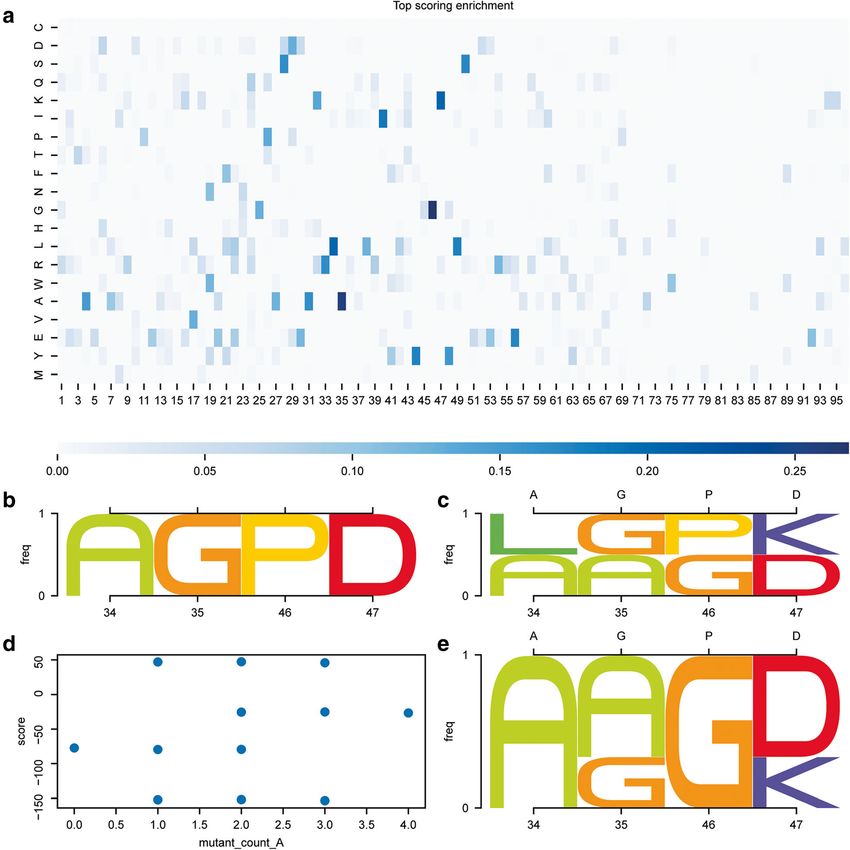
from rstoolbox are highlighted in bold. Styling commands are skipped to facilitate reading, but can be found in the repository’s notebook.Bonet et al. BMC Bioinformatics (2019) 20:240 Page 7 of 13 Guiding iterative CPD workflows The rstoolbox presents a diversity of functions that Many CPD workflows rely on iterative approaches in aid this process and perform tasks from selecting decoys which multiple rounds of design are performed and each with specific mutations of interest, to those that define generation of designs is used to guide the next one. residue sets for instance based in position weight matrices Fig. 3 Guiding iterative design pipelines. Information retrieved from decoy populations can be used to guide following generations of designs. With the exception of the panel identifiers, the image was directly created with the code presented in Table 2. a Mutant enrichment from comparison of the design on top 5% by score and the overall population. Positions 34, 35, 46 and 47 present a 20% enrichment of certain residue types over the whole population and are selected as positions of interest. b Residue types for the positions of interest in the decoy selected as template of the second generation. c Upon guided mutagenesis, we obtain a total of 16 decoys including the second-generation template. We can observe that the overrepresented residues shown in A are now present in the designed population. Upper x axis shows the original residue types of the template. d Combinatorial targeted mutagenesis yields 16 new designs, three of which showed an improved total score relative to the second-generation template (mutant_count_A is 0). e The three best scoring variants show mutations such as P46G which seem to be clearly favorable for the overall score of the designs. Upper x axis shows the original residue types of the template
Bonet et al. BMC Bioinformatics (2019) 20:240 Page 8 of 13
(generate_mutants_from_matrix()). When rede- sequence design [28]. FunFolDes was developed to insert
signing naturally occurring proteins, it also presents a functional sites into protein scaffolds and allow for
function to generate reversions to wild-type residues full-backbone flexibility to enhance sequence sampling. As
(generate_wt_reversions()) to generate the best a demonstration of its performance, we designed a new
possible design with the minimal number of mutations. protein to serve as an epitope-scaffold for the Respiratory
These functions will directly execute Rosetta, if installed Syncytial Virus site II (PDB ID: 3IXT [29]), using as
in the system, but can also be used to create input files to scaffold the A6 protein of the Antennal Chemosensory
run the simulations in different software suits. Code ex- system from Mamestra brassicae (PDB ID: 1KX8 [30]).
ample for these functionalities is shown in Table 2. The The designs were obtained in a two-stage protocol, with
result of the code is depicted on Fig. 3. the second generation being based on the optimization of
rstoolbox allows the user to exploit the data ob- a small subset of first-generation decoys. The code pre-
tained from the analysis of designed populations in order sented in Table 3 shows how to process and compare the
to bias following design rounds. When using rstool- data of both generations. Extra plotting functions to rep-
box, this process is technically simple and clear to other resent experimental data obtained from the biochemical
users, which will improve the comprehension and repro- characterization of the designed proteins is also shown.
ducibility of iterative design pipelines. The result of this code is represented in Fig. 4.
Evaluation of designed proteins Benchmarking design protocols
Recently, we developed the Rosetta FunFolDes protocol, One of the main novelties of FunFolDes was the ability
which was devised to couple conformational folding and to include a binding partner during the folding-design
Table 3 Sample code for the evaluation of a multistep design pipeline
Action Code Sample
Load import rstoolbox as rs
import matplotlib.pyplot as plt
Read # With Rosetta installed, scoring can be run for a single structure
baseline = rs.io.get_sequence_and_structure(‘1kx8.pdb’, minimize = True)
slen = len(baseline.iloc[0].get_sequence(‘A’))
# Pre-calculated sets can also be loaded to contextualize the data
# 70% homology filter
cath = rs.utils.load_refdata(‘cath’, 70)
# Length in a window of 10 residues around expected design length
cath = cath[(cath[‘length’] > = slen - 5) & (cath[‘length’] < = slen + 5)]
# Designs were performed in two rounds
gen1 = rs.io.parse_rosetta_file(‘1kx8_gen1.designs’)
gen2 = rs.io.parse_rosetta_file(‘1kx8_gen2.designs’)
# Identifiers of selected decoys:
decoys = [‘d1’, ‘d2’, ‘d3’, ‘d4’, ‘d5’, ‘d6’]
# Load experimental data for d2 (best performing decoy)
df_cd = rs.io.read_CD(‘1kx8_d2/CD’, model = ‘J-815’)
df_spr = rs.io.read_SPR(‘1kx8_d2/SPR.data’)
Plot fig = plt.figure(figsize = (170 / 25.4, 170 / 25.4))
grid = (3, 4)
# Compare scores between the two generations
axs = rs.plot.multiple_distributions(gen2, fig, (3, 4), values = [‘score’, ‘hbond_bb_sc’, ‘hbond_sc’,
‘rmsd’], refdata = gen1, violins = False, showfliers = False)
# See how the selected decoys fit into domains of similar size
qr = gen2[gen1[‘description’].isin(decoys)]
axs = rs.plot.plot_in_context(qr, fig, (3, 2), cath, (1, 0), [‘score’, ‘cav_vol’])
axs[0].axvline(baseline.iloc[0][‘score’], color = ‘k’, linestyle = ‘--’)
axs[1].axvline(baseline.iloc[0][‘cavity’], color = ‘k’, linestyle = ‘--’)
# Plot experimental validation data
ax = plt.subplot2grid(grid, (2, 0), fig = fig, colspan = 2)
rs.plot.plot_CD(df_cd, ax, sample = 7)
ax = plt.subplot2grid(grid, (2, 2), fig = fig, colspan = 2)
rs.plot.plot_SPR(df_spr, ax, fitcolor = ‘black’)
plt.tight_layout()
plt.savefig(‘BMC_Fig4.png’, dpi = 300)
The code shows how to combine the data from multiple Rosetta simulations and assess the different features between two design populations in terms of
scoring as well as the comparison between the final designs and the initial structure template. Code comments are presented in italics while functions from the
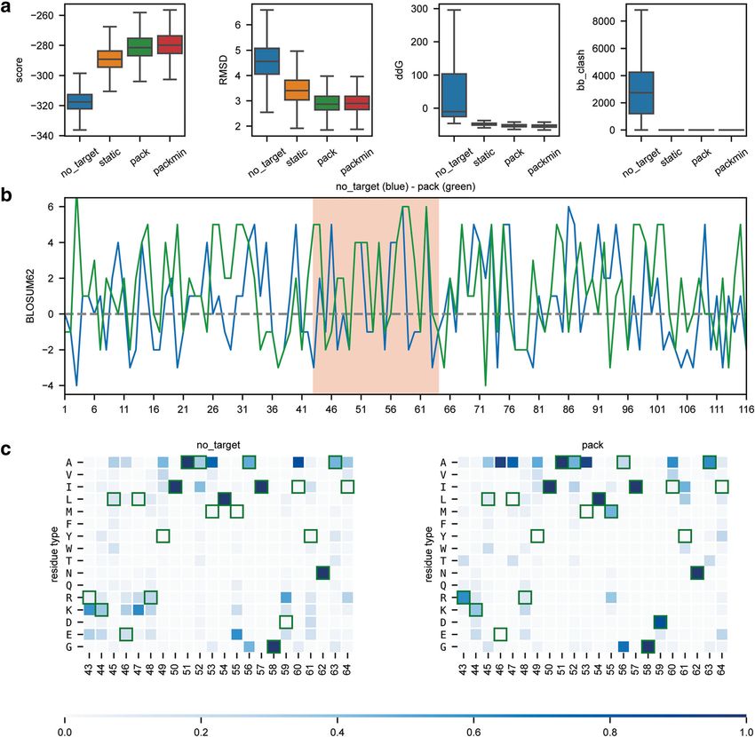
rstoolbox are highlighted in bold. Styling commands are skipped to facilitate reading, but can be found in the repository’s notebook.Bonet et al. BMC Bioinformatics (2019) 20:240 Page 9 of 13 Fig. 4 Multi-stage design, comparison with native proteins and representation of experimental data for 1kx8-based epitope-scaffold. Analysis of the two-step design pipeline, followed by a comparison of the distributions obtained for native proteins and the designs and plotting of biochemical experimental data. With the exception of the panel identifiers, the image was directly created with the code presented in Table 3. a Comparison between the first (orange) and the second (blue) generation of designs. score – shows the Rosetta energy score; hbond_bb_sc – quantifies the hydrogen bonds between backbone and side chain atoms; hbond_sc - quantifies the hydrogen bonds occurring between side chain atoms; RMSD – root mean square deviation relative to the original template. Second-generation designs showed minor improvements on backbone hydrogen bonding and a substantial improvement in overall Rosetta Energy. b Score and cavity volume for the selected decoys in comparison with structures of CATH [31] domains of similar size. The vertical dashed black line represents the score and cavity volume of the original 1kx8 after minimization, highlighting the improvements relative to the original scaffold. c Circular Dichroism and Surface Plasmon Resonance data for the best design shows a well folded helical protein that binds with high affinity to the expected target simulations. This feature allows to bias the design simu- benchmark test the previously computationally designed lations towards productive configurations capable of protein BINDI, a 3-helix bundle that binds to BHRF1 properly displaying the functional motif transplanted to [32]. We performed simulations under four different the scaffold. To assess this new feature, we used as a conditions: no-target (binding-target absent), static
Bonet et al. BMC Bioinformatics      (2019) 20:240                                                                                     Page 10 of 13

(binding-target without conformational freedom), pack                       populations performed regarding energetic sampling
(binding-target with side-chain repacking) and packmin                      (Fig. 5a) and the mimicry of BINDI’s conformational
(binding-target with side chain repacking and backbone                      shift from the original scaffold (Fig. 5a). In addition,
minimization) and evaluated the performance of each                         we quantified the sequence recovery relative to the
simulation. Specifically, we analysed how the design                        experimentally characterized BINDI sequence (Fig. 5b

 Fig. 5 Comparison and benchmarking of different design protocols. Representation of the results obtained using four different design protocols.
 With the exception of the panel identifiers, the image was directly created with the code presented in Table 4. a Representation of four scoring
 metrics in the design of a new protein binder. score – shows the overall Rosetta score; RMSD – root mean square deviation relative to BINDI;
 ddG –Rosetta energy for the interaction between two proteins; bb_clash - quantifies the backbone clashes between the binder and the target
 protein; b BLOSUM62 positional sequence score for the top design of the no_target (blue) and pack (green) design populations showcases how
 to analyse and compare individual decoys. The higher the value, the more likely two residue types (design vs. BINDI) are to interchange within
 evolutionary related proteins. Special regions of interest can be easily highlighted, as for instance the binding region (highlighted in salmon). c
 Population-wide analysis of the sequence recovery of the binding motif region for no_target and pack simulations. Darker shades of blue indicate
 a higher frequency and green frames indicate the reference residue type (BINDI sequence). This representation shows that the pack population
 explores more frequently residue types found in the BINDI design in the region of the binding motif
Bonet et al. BMC Bioinformatics        (2019) 20:240                                                                                           Page 11 of 13

and c). Table 4 exemplifies how to easily load and combine                       where one can alter and improve the activity and stability
the generated data and create a publication-ready com-                           of newly engineered proteins for a number of important
parative profile between the four different approaches                           applications. In the age of massive datasets, structural data
(Fig. 5).                                                                        is also quickly growing both through innovative experi-
                                                                                 mental approaches and more powerful computational
Discussion                                                                       tools. To deal with fast-growing amounts of structural
The analysis of protein structures is an important ap-                           data, new analysis tools accessible to users with
proach to enable the understanding of fundamental bio-                           beginner-level coding experience are urgently needed.
logical processes, as well as, to guide design endeavours                        Such tools are also enabling for applications in CPD,

Table 4 Sample code for the comparison between 4 different decoy populations
Action   Code Sample
Load     import pandas as pd
         import rstoolbox as rs
         import matplotlib.pyplot as plt
Read     df = []
         # With Rosetta installed, scoring can be run for a single structure
         baseline = rs.io.get_sequence_and_structure(‘4yod.pdb’)
         experiments = [‘no_target’, ‘static’, ‘pack’, ‘packmin’]
         scores = [‘score’, ‘LocalRMSDH’, ‘post_ddg’, ‘bb_clash’]
         scorename = [‘score’, ‘RMSD’, ‘ddG’, ‘bb_clash’]
         for experiment in experiments:
             # Load Rosetta silent file from decoy generation
             ds = rs.io.parse_rosetta_file(experiment + ‘.design’)
             # Load decoy evaluation from a pre-processed CSV file.
             # Casting pd. DataFrame into DesignFrame is as easy as shown here.
             ev = rs.components. DesignFrame(pd.read_csv(experiment + ‘.evals’))
             # Different outputs for the same decoys can be combined through
             # their ‘description’ field (decoy identifier)
             df.append(ds.merge (ev, on = ‘description’))
             # Tables can be joined together into a single working object
             df = pd.concat(df)
             # As we are comparing over BINDI’s sequence, that is our reference.
             df.add_reference_sequence(‘B’, baseline.iloc[0].get_sequence(‘B’)[:-1])
Plot     fig = plt.figure (figsize = (170 / 25.4, 170 / 25.4))
         grid = (12, 4)
         # Show the distribution for key score terms
         axs = rs.plot.multiple_distributions(df, fig, grid, values = scores, rowspan = 3,
               labels = scorename, x = ‘binder_state’, order = experiments, showfliers = False)
         # Sequence score for a selected decoys with standard-matrix weights
         ax = plt.subplot2grid(grid, (3, 0), fig = fig, colspan = 4, rowspan = 4)
         qr = df[df[‘binder_state’] == ‘no_target’].sort_values(‘score’).iloc[0]
         rs.plot.per_residue_matrix_score_plot(qr, ‘B’, ax, ‘BLOSUM62’, add_alignment = False, color = 0)
         qr = df[df[‘binder_state’] == ‘no_pack’].sort_values(‘score’).iloc[0]
         rs.plot.per_residue_matrix_score_plot(qr, ‘B’, ax, ‘BLOSUM62’, add_alignment = False, color = 2,
                                                   selections = [(‘43–64’, ‘red’)])
         # Small functions help edit the plot display
         rs.utils.add_top_title(ax, ‘no_target (blue) - pack (green)’)
         # Evaluate the variability of residue types in the binding region
         ax = plt.subplot2grid(grid, (7, 0), fig = fig, colspan = 2, rowspan = 4)
         qr = df[df[‘binder_state’] == ‘no_target’]
         rs.plot.sequence_frequency_plot(qr, ‘B’, ax, key_residues = ‘43–64’, cbar = False, clean_unused = 0.1,
         xrotation = 90)
         rs.utils.add_top_title(ax, ‘no_target’)
         ax = plt.subplot2grid(grid, (7, 2), fig = fig, colspan = 2, rowspan = 4)
         ax_cbar = plt.subplot2grid(grid, (11, 0), fig = fig, colspan = 4)
         rs.plot.sequence_frequency_plot(df[df[‘binder_state’] == ‘pack’], ‘B’, ax, key_residues = ‘43–64’,
                                            cbar_ax = ax_cbar, clean_unused = 0.1, xrotation = 90)
         rs.utils.add_top_title(ax, ‘pack’)
         plt.tight_layout()
         plt.savefig(‘BMC_Fig5.png’, dpi = 300)
The code shows how to join data from multiple Rosetta experiments to assess the key difference between four design populations in terms of different scoring
metrics and sequence recovery. Code comments are presented in italics while functions from the rstoolbox are highlighted in bold. Styling commands are
skipped to facilitate reading, but can be found in the repository’s notebook.
Bonet et al. BMC Bioinformatics (2019) 20:240 Page 12 of 13
where large amounts of structural and sequence data are Abbreviations
routinely generated. Here, we describe and exemplify the CPD: Computational protein design; FunFolDes: Rosetta functional folding
and design; RMSD: Root Mean square deviation
usage of rstoolbox to analyse CPD data illustrating
how these tools can be used to distil large structural data- Acknowledgements
sets and produce intuitive graphical representations. We would like to thank all the members of the LPDI who have acted as
beta-testers of the code, reporting bugs and suggesting new features.
CPD approaches are becoming more popular and
achieving important milestones in generating proteins Funding
with novel functions [1]. However, CPD pipelines remain JB is sponsored by an EPFL-Fellows grant funded by an H2020 MSC action.
FS is funded by the Swiss Systemsx.ch initiative. BEC is a grantee from the
technically challenging with multiple design and selec-
ERC [starting grant – 716058], the SNSF and the Biltema Foundation. The
tion stages which are different for every design problem funding bodies played no role in the design of the study, analysis,
and thus often require user intervention. Within the ap- interpretation of data or in writing the manuscript.
plications of rstoolbox, several functionalities can aid
Availability of data and materials
in this process, by providing an easy programmatic inter- All the examples presented in this work including a basic structural
face to perform selections, comparisons with native pro- bioinformatics application, can be reproduced following the two IPython
teins, graphical representations and informing follow-up notebooks present at https://mybinder.org/v2/gh/lpdi-epfl/rstoolbox/
51ccd51?filepath=notebook
rounds of design in iterative, multi-step protocols. The tools The rstoolbox can be directly installed through PyPI and the source code is
presented here were devised for Rosetta CPD calculations, freely available at https://github.com/lpdi-epfl/rstoolbox, with a full
nevertheless the table-like data structure used allows for documentation available at https://lpdi-epfl.github.io/rstoolbox. All
requirements for the basic workings of the library are obtained via PyPI.
the easy creation of parsers for other protein modelling and
design tools. This is especially relevant in other modelling Authors’ contributions
protocols that require large sampling such as protein dock- JB, ZH, FS and AS contributed to the code. JB and BEC devised the examples
and wrote the manuscript. All authors read, contributed and approved the
ing [33]. Importantly, rstoolbox can also be useful for final version of the manuscript.
structural bioinformatics and the analysis of structural fea-
tures which have become more enlightening with the Ethics approval and consent to participate
Not applicable.
growth of different structural databases (e.g. PDB [34],
SCOP [35], CATH [31]). Consent for publication
Not applicable.
Conclusion Competing interests
Here, we present the rstoolbox, a Python library for The authors’ declare that they have no competing interests.
the analysis of large-scale structural data tailored for
CPD applications and adapted to a wide variety of user Publisher’s Note
Springer Nature remains neutral with regard to jurisdictional claims in published
expertise. We endowed rstoolbox with an extensive
maps and institutional affiliations.
documentation and a continuous integration setup to
ensure code stability. Thus, rstoolbox can be Received: 23 January 2019 Accepted: 8 April 2019
accessed and expanded by users with beginner’s level
programming experience guaranteeing backward References
compatibility. The inclusion of rstoolbox in design, 1. Gainza-Cirauqui P, Correia BE. Computational protein design-the next
protocol development and structural bioinformatics generation tool to expand synthetic biology applications. Curr Opin
Biotechnol. 2018;52:145–52.
pipelines will aid in the comprehension of the 2. Taylor WR, Chelliah V, Hollup SM, MacDonald JT, Jonassen I. Probing the
human-guided decisions and actions taken during the "dark matter" of protein fold space. Structure. 2009;17(9):1244–52.
processing of large structural datasets, helping to ensure 3. Pierce NA, Winfree E. Protein design is NP-hard. Protein Eng. 2002;15(10):
779–82.
their reproducibility. 4. Gainza P, Roberts KE, Georgiev I, Lilien RH, Keedy DA, Chen CY, et al.
OSPREY: protein design with ensembles, flexibility, and provable algorithms.
Methods Enzymol. 2013;523:87–107.
Availability and requirements 5. Chen CY, Georgiev I, Anderson AC, Donald BR. Computational structure-
Project name: rstoolbox. based redesign of enzyme activity. Proc Natl Acad Sci U S A. 2009;106(10):
3764–9.
Project home page: https://lpdi-epfl.github.io/rstoolbox 6. Frey KM, Georgiev I, Donald BR, Anderson AC. Predicting resistance
Operating system(s): Tested on Linux and macOS. mutations using protein design algorithms. Proc Natl Acad Sci U S A. 2010;
Programming language: Python. 107(31):13707–12.
7. Bolon DN, Mayo SL. Enzyme-like proteins by computational design. Proc
Other requirements: python2.7 or python3.4+. Non- Natl Acad Sci U S A. 2001;98(25):14274–9.
standard Python libraries required are automatically in- 8. Dahiyat BI, Mayo SL. De novo protein design: fully automated sequence
stalled during setup with pip. selection. Science. 1997;278(5335):82–7.
9. Shimaoka M, Shifman JM, Jing H, Takagi J, Mayo SL, Springer TA.
License: MIT. Computational design of an integrin I domain stabilized in the open high
Any restrictions to use by non-academics: None. affinity conformation. Nat Struct Biol. 2000;7(8):674–8.Bonet et al. BMC Bioinformatics (2019) 20:240 Page 13 of 13
10. Li Z, Scheraga HA. Monte Carlo-minimization approach to the multiple-
minima problem in protein folding. Proc Natl Acad Sci U S A. 1987;84(19):
6611–5.
11. Gainza P, Nisonoff HM, Donald BR. Algorithms for protein design. Curr Opin
Struct Biol. 2016;39:16–26.
12. Alford RF, Leaver-Fay A, Jeliazkov JR, O'Meara MJ, DiMaio FP, Park H, et al.
The Rosetta all-atom energy function for macromolecular modeling and
design. J Chem Theory Comput. 2017;13(6):3031–48.
13. Simons KT, Bonneau R, Ruczinski I, Baker D. Ab initio protein structure
prediction of CASP III targets using ROSETTA. Proteins. 1999;Suppl 3:171–6.
14. Kim DE, Blum B, Bradley P, Baker D. Sampling bottlenecks in de novo
protein structure prediction. J Mol Biol. 2009;393(1):249–60.
15. Kuhlman B, Baker D. Native protein sequences are close to optimal for their
structures. Proc Natl Acad Sci U S A. 2000;97(19):10383–8.
16. Rosetta Commons. Rosetta Tools: https://www.rosettacommons.org/docs/
latest/application_documentation/tools/Tools. 2018.
17. Pérez F, Granger EB. IPython: a system for interactive scientific computing.
Comput Sci Eng. 2007;9(3):21–9.
18. McKinney W. Data structures for statistical computing in Python. In:
Proceedings of the 9th Python in science conference; 2010. p. 51–6.
19. Schneider TD, Stephens RM. Sequence logos: a new way to display
consensus sequences. Nucleic Acids Res. 1990;18(20):6097–100.
20. Ramachandran GN, Ramakrishnan C, Sasisekharan V. Stereochemistry of
polypeptide chain configurations. J Mol Biol. 1963;7:95–9.
21. Thompson JD, Gibson TJ, Higgins DG. Multiple sequence alignment using
ClustalW and ClustalX. Curr Protoc Bioinformatics. 2002;00(1):2.3.1-2.3.22.
Chapter 2:Unit 2 3.
22. Potter SC, Luciani A, Eddy SR, Park Y, Lopez R, Finn RD. HMMER web server:
2018 update. Nucleic Acids Res. 2018;46(W1):W200–W4.
23. Hunter JD. Matplotlib: a 2D graphics environment. Comput Sci Eng. 2007;
9(3):90–5.
24. Michael Waskom OB, Drew O'Kane, Paul Hobson, Joel Ostblom, Saulius
Lukauskas, Adel Qalieh. mwaskom/seaborn: v0.9.0 Zenodo. 2018.
25. Stein A, Kortemme T. Improvements to robotics-inspired conformational
sampling in rosetta. PLoS One. 2013;8(5):e63090.
26. Kuhlman B, Dantas G, Ireton GC, Varani G, Stoddard BL, Baker D. Design of a
novel globular protein fold with atomic-level accuracy. Science. 2003;
302(5649):1364–8.
27. Marcos E, Basanta B, Chidyausiku TM, Tang Y, Oberdorfer G, Liu G, et al.
Principles for designing proteins with cavities formed by curved beta
sheets. Science. 2017;355(6321):201–6.
28. Bonet J, Wehrle S, Schriever K, Yang C, Billet A, Sesterhenn F, et al. Rosetta
FunFolDes - a general framework for the computational design of
functional proteins. PLoS Comput Biol. 2018;14(11):e1006623.
29. McLellan JS, Chen M, Kim A, Yang Y, Graham BS, Kwong PD. Structural basis
of respiratory syncytial virus neutralization by motavizumab. Nat Struct Mol
Biol. 2010;17(2):248–50.
30. Lartigue A, Campanacci V, Roussel A, Larsson AM, Jones TA, Tegoni M, et al.
X-ray structure and ligand binding study of a moth chemosensory protein. J
Biol Chem. 2002;277(35):32094–8.
31. Sillitoe I, Dawson N, Lewis TE, Das S, Lees JG, Ashford P, et al. CATH:
expanding the horizons of structure-based functional annotations for
genome sequences. Nucleic Acids Res. 2018;47(D1):D280–4.
32. Procko E, Berguig GY, Shen BW, Song Y, Frayo S, Convertine AJ, et al. A
computationally designed inhibitor of an Epstein-Barr viral Bcl-2 protein
induces apoptosis in infected cells. Cell. 2014;157(7):1644–56.
33. Coleman RG, Carchia M, Sterling T, Irwin JJ, Shoichet BK. Ligand pose and
orientational sampling in molecular docking. PLoS One. 2013;8(10):e75992.
34. Berman HM, Westbrook J, Feng Z, Gilliland G, Bhat TN, Weissig H, et al. The
protein data Bank. Nucleic Acids Res. 2000;28(1):235–42.
35. Andreeva A, Howorth D, Chandonia JM, Brenner SE, Hubbard TJ, Chothia C,
et al. Data growth and its impact on the SCOP database: new
developments. Nucleic Acids Res. 2008;36(Database issue):D419–25.You can also read