Monte-Carlo Tree Search for Efficient Visually Guided Rearrangement Planning
←
→
Page content transcription
If your browser does not render page correctly, please read the page content below
Monte-Carlo Tree Search for Efficient
                                                                       Visually Guided Rearrangement Planning
                                                                 Yann Labbé a,b , Sergey Zagoruyko a,b , Igor Kalevatykh a,b , Ivan Laptev a,b ,
                                                                       Justin Carpentier a,b , Mathieu Aubry c and Josef Sivic a,b,d

                                           Abstract— We address the problem of visually guided rear-                              (a)                               (b)
                                        rangement planning with many movable objects, i.e., finding
                                        a sequence of actions to move a set of objects from an initial
                                        arrangement to a desired one, while relying on visual inputs
arXiv:1904.10348v2 [cs.RO] 1 Apr 2020

                                        coming from an RGB camera. To do so, we introduce a
                                        complete pipeline relying on two key contributions. First, we
                                        introduce an efficient and scalable rearrangement planning
                                        method, based on a Monte-Carlo Tree Search exploration
                                        strategy. We demonstrate that because of its good trade-off
                                        between exploration and exploitation our method (i) scales well
                                        with the number of objects while (ii) finding solutions which
                                        require a smaller number of moves compared to the other
                                                                                                                                                                    (d)
                                        state-of-the-art approaches. Note that on the contrary to many
                                        approaches, we do not require any buffer space to be available.
                                        Second, to precisely localize movable objects in the scene,                       ...
                                        we develop an integrated approach for robust multi-object
                                        workspace state estimation from a single uncalibrated RGB
                                        camera using a deep neural network trained only with synthetic                               ...
                                        data. We validate our multi-object visually guided manipulation
                                        pipeline with several experiments on a real UR-5 robotic arm
                                                                                                                           (c)
                                        by solving various rearrangement planning instances, requiring
                                        only 60 ms to compute the plan to rearrange 25 objects. In                  Fig. 1: Visually guided rearrangement planning. Given a source
                                        addition, we show that our system is insensitive to camera move-            (a) and target (b) RGB images depicting a robot and multiple
                                        ments and can successfully recover from external perturbations.             movable objects, our approach estimates the positions of objects
                                        Supplementary video, source code and pre-trained models are                 in the scene without the need for explicit camera calibration and
                                        available at https://ylabbe.github.io/rearrangement-planning.               efficiently finds a sequence of robot actions (c) to re-arrange the
                                                                                                                    scene into the target scene. Final object configuration after re-
                                                                I. I NTRODUCTION                                    arrangement by the robot is shown in (d).
                                                                                                                    target one. The current and target states are described only
                                           Using a robot to clean up a room is a dream shared far
                                                                                                                    by a single image taken from an uncalibrated RGB camera.
                                        beyond the robotics community. This would require a robot
                                                                                                                       Rearrangement planning has a long history in robotics
                                        to both localize and re-arrange many objects. Other industrial
                                                                                                                    [1]–[6] and remains an active research topic [7]–[10] in the
                                        scenarios, such as sorting and packing objects on a pro-
                                                                                                                    motion planing community. The goal is to find a sequence
                                        duction line or car assembly tasks, share similar objectives
                                                                                                                    of transit and transfer motions [1,5] to move a set of
                                        and properties. This paper presents an integrated approach
                                                                                                                    objects from an initial arrangement to a target arrangement,
                                        that makes a step towards the efficiency, scalability and
                                                                                                                    while avoiding collisions with the environment. This leads
                                        robustness required for solving such rearrangement planning
                                                                                                                    to a complex sequential decision process, whose complexity
                                        tasks. Fig. 1 shows an example of the problem we consider,
                                                                                                                    depends on the number of objects to move, on the free-space
                                        where objects have to be moved from an initial position to a
                                                                                                                    available around the objects, and the robot kinematics.
                                                                                                                       Several solutions have been proposed in the literature
                                           This work was partially supported by the DGA RAPID projects DRAAF
                                        and TABASCO, the MSR-Inria joint lab, the Louis Vuitton - ENS Chair         which can be roughly classified into two groups. Methods
                                        on Artificial Intelligence, the HPC resources from GENCI-IDRIS (Grant       in the first group [6,8]–[12] rely on the task and motion
                                        011011181), the ERC grant LEAP (No. 336845), the CIFAR Learning             planning hierarchy where a high-level task planner is com-
                                        in Machines&Brains program, the European Regional Development Fund
                                        under the project IMPACT (reg. no. CZ.02.1.01/0.0/0.0/15 003/0000468)       bined with a local motion planner [3]. Methods in the second
                                        and the French government under management of Agence Nationale de           group [2,4,13,14] aim at solving a single unified formulation
                                        la Recherche as part of the ”Investissements d’avenir” program, reference   of the problem by using classic sample-based algorithms
                                        ANR-19-P3IA-0001 (PRAIRIE 3IA Institute).
                                           a Département d’informatique de l’ENS, École normale supérieure,      such as Probabilistic RoadMap (PRM) or Rapidly-Exploring
                                        CNRS, PSL Research University, 75005 Paris, France, b INRIA,                Random Tree (RRT) [3] or use advanced optimization strate-
                                        France,c LIGM (UMR 8049), École des Ponts, UPE, France,d Czech Institute   gies to solve a unique optimization instance [15].
                                        of Informatics, Robotics and Cybernetics, Czech Technical University in
                                        Prague.                                                                        While methods from both groups have been shown to
                                           Corresponding author: yann.labbe@inria.fr                                work well in practice with few objects, existing methods do
target
                                               state                        the workspace. The last stage is a standard RRT-based local
                                                                            motion planner which plans robot movements given the high-
             Visual state     state    MCTS
              prediction              Task Planner
                                                                RRT         level plan computed by the MCTS planner.
                                                           Motion Planner
               (section IV)            (section III)

                                                  planning                                       II. R ELATED WORK
              image           Environment              action
                                   +                                           We build our framework on results in robotics, search
                                 Robot                                      algorithms and computer vision, which we review below.
Fig. 2: Approach overview. Given an image of the scene, the                 Rearrangement planning is NP-hard [21]. As a result, stan-
visual state prediction module outputs a list of objects and their          dard hierarchical [6,8,9,12] and randomized methods [2,4,14]
coordinates in the robot coordinate frame. Together with a target           for solving general manipulation planning problems do not
state, these serve as inputs to the task and motion planning module         scale well with the number of objects. The most efficient and
which combines Monte-Carlo Tree Search with a standard robot
motion planning algorithm.                                                  scalable high-level planners only address specific constrained
                                                                            set-ups leveraging the structure of the rearrangement problem
not scale to a large set of objects, because the number of                  [8,10,13]. In addition, they often focus on feasibility but do
possible action sequences increases exponentially with the                  not attempt to find high-quality solutions with a low number
number of objects to move. Some recent methods [8,10,13]                    of object moves [8,13]. For instance, some methods [13] only
scale better with the number of objects but these methods                   consider the monotone problem instances, where each object
either only focus on feasibility, producing solutions with                  can be grasped at most once. In contrast, our method finds
sub-optimal number of grasps [8], or are limited to specific                high-quality plans but also addresses the more general cases
constrained scenarios, for example, with explicitly available               of non-monotone re-arrangement problems, which are known
buffer space [10] or strict constraints of monotony (i.e. an                to be significantly harder [4]. Others works have looked at
object can be moved only once during the plan).                             finding optimal plans [10] but address only constrained set-
   In this work we describe an efficient and generic approach               ups that have available buffer space (i.e. space that does not
for rearrangement planning that overcomes these limitations:                overlap with the union of the initial and target configura-
(i) it scales well with the number of objects, by taking                    tions), noting that solving the general case without available
only 60 ms to plan complex rearrangement scenarios for                      buffer space is significantly harder [10]. In this work, we
multiple objects, and (ii) it can be applied to the most                    address this more general case and describe an approach
challenging table-top re-arrangement scenarios, not requiring               that efficiently finds high-quality re-arrangement solutions
explicit buffer space. Our approach is based on Monte-Carlo                 without requiring any available buffer space. In addition and
Tree Search [16], which allows us to lower the combina-                     unlike previous works [8,10,13], we also propose a complete
torial complexity of the decision process and to find an                    system able to operate from real images in closed loop.
optimistic number of steps to solve the problem, by making                     Search algorithms. The problem of rearrangement plan-
a compromise between exploration (using random sampling)                    ning can be posed as a tree search. Blind tree search
and exploitation (biasing the search towards the promising                  algorithms such as Breadth-First search (BFS) [22] can be
already sampled action sequences to cut off some of the                     used to iteratively expand nodes of a tree until a goal node
search directions).                                                         is found, but these methods do not exploit information about
   To demonstrate the benefits of our planning approach in                  the problem (e.g. a cost or reward) to select which nodes
real scenarios we also introduced a multi-object calibration-               to expand first, and typically scale exponentially with the
free deep neural network architecture for object position                   tree depth. Algorithms such as greedy BFS [22] allow to
estimation. It is trained entirely from synthetic images and,               exploit a reward function to drive the exploration of the
compared to other currently available methods [17]–[20],                    tree directly towards nodes with high reward, but might
does not use markers or require known CAD models of                         get stuck in a local mimima. Other algorithms such as
the specific observed object instances. To the best of our                  A? [23] can better estimate the promising branches using
knowledge, the approach we present is the first one able                    additional hand-crafted heuristic evaluation function. We
to locate multiple objects in such difficult and generic                    choose Monte-Carlo Tree Search over others, because it only
conditions. This is of high practical interest, since it allows             relies on a reward and iteratively learns a heuristic (the
to perform the full task using only a single non-calibrated,                value function) which allows to efficiently balance between
or even hand-held, RGB camera looking at the robot.                         exploration and exploitation. It has been used in related areas
   Our complete pipeline for visually guided rearrangement                  to solve planning and routing for ground transportation [24]
planning, illustrated in Fig. 2, is composed of three main                  and to guide the tree-search in cooperative manipulation [25].
stages. The goal of the first stage, visual state prediction                MCTS is also at the core of AlphaGo, the first system able to
(section III), is to estimate the positions of multiple objects             achieve human performance in the game of Go [26], where it
relative to a robot given a single non-calibrated image of the              was combined with neural networks to speed-up the search.
scene. The second stage (Sec. IV), is our MCTS-based task                   These works directly address problems whose action space
planner: at each planning step, this module chooses which                   is discrete by nature. In contrast, the space of possible object
object to move and computes its new desired position in                     arrangements is infinite. We propose a novel discrete action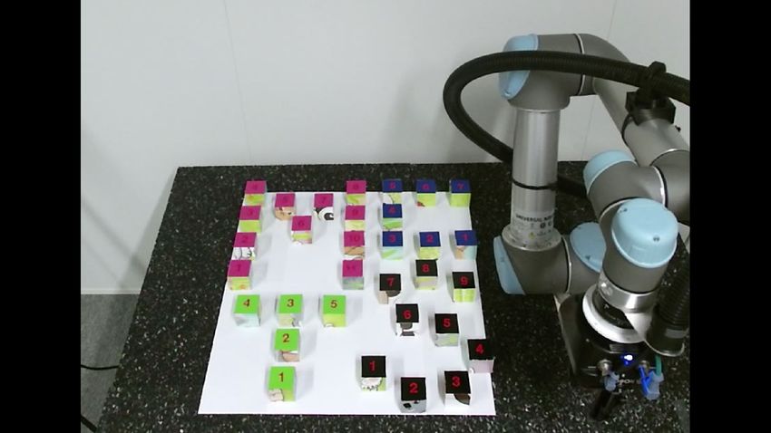
parameterization of the rearrangement planning problem             A. Position prediction network
which allows us to efficiently apply MCTS.                            In this section, we give details of the network for pre-
Vision-based object localization. In robotics, fiducial mark-      dicting a dense 2D position field and an object segmentation
ers are commonly used for detecting the objects and pre-           mask. The 2D position field maps each input pixel to a 2D
dicting their pose relative to the camera [17] but their use       coordinate frame of the robot acting as implicit calibration.
limits the type of environments the robot can operate in. This     Architecture. Our architecture is based on ResNet-34 [36].
constraint can be removed by using a trainable object detec-       We remove the average pooling and fully connected layers
tor architecture [18]–[20,27]–[29]. However, these methods         and replace them by two independent decoders. Both de-
often require gathering training data for the target objects       coders use the same architecture: four transposed convolution
at hand, which is often time consuming and requires the            layers with batch normalization and leaky ReLU activations
knowledge of the object (e.g. in the form its 3D model)            in all but the last layer. The resolution of the input image is
beforehand. In addition, these methods estimate the pose           320 × 240 and the spatial resolution of the output of each
of the objects in the frame of the camera and using these          head is 85 × 69. We add the 6D joint configuration vector
predictions for robotic manipulation requires calibration of       of the robot as input to the network by copying it into a
the camera system with respect to the robot. The calibration       tensor of size 320 × 240 × 6, and simply concatenating it
procedure [30,31] is time-consuming and must be redone             with the three channels of the input image. The two heads
each time the camera is moved. More recently, [32] proposed        predict an object mask and a 2D position field which are
to directly predict the position of a single object in the robot   visualized in Fig. 3. In addition, we found that predicting
coordinate frame by training a deep network on hundreds of         depth and semantic segmentation during training increased
thousands of synthetically generated images using domain           the localization accuracy at test time. These modalities are
randomization [32]–[35]. We build on the work [32] and             predicted using two additionnal decoders with the same
extend it for predicting the 2D positions of multiple objects      architecture.
with unknown dimensions relative to the robot.                     Synthetic training data. Following [32]–[35], we use do-
                                                                   main randomization for training our network without requir-
 III. V ISUAL SCENE STATE PREDICTION WITH MULTIPLE
                                                                   ing any real data. We generate two million images displaying
                           OBJECTS
                                                                   the robot and a variable number of objects with various
   In this section, we detail the visual state prediction stage.   shapes (cubes, cylinders and triangles) in its workspace. In
Our visual system takes as input a single photograph of            each scene, we randomly sample from 1 up to 12 objects,
a scene taken from an uncalibrated camera and predicts a           with various dimensions between 2.5 and 8 cm. Examples
workspace state that can then be used for rearrangement-           of training images are shown in Fig. 4. Randomization
planning. More precisely it outputs the 2D positions of            parameters include the textures of the robot and objects, the
a variable number of objects expressed in the coordinate           position of the gripper, the position, orientation and field of
system of the robot. This problem is difficult because the         view of the camera, the positions and intensities of the light
scene can contain a variable number of objects, placed on          sources and their diffuse/ambient/specular coefficients.
different backgrounds, in variable illumination conditions,        Training procedure. We train our network by minimizing
and observed from different viewpoints, as illustrated in          the following loss: L = Lpos +Lmask +Lsegm +Ldepth , where
Fig. 1. In contrast to [33], we do not assume that the different   the individual termsP    are explained    next. For the position field
types of objects are known at training time. In contrast to

                                                                   loss we use Lpos = i,j δi,j (x̂i,j − xi,j )2 + (ŷi,j − yi,j )2
state-of-the-art pose estimation techniques in RGB images          where (i, j) are the pixel coordinates in the output; δi,j
[17,18], we do not use markers and do not assume the CAD           is the binary object mask; xi,j , yi,j are the ground truth
models of the objects are known at test time.                      2D coordinates of the center of the object (that appears at
   To address these challenges, we design a visual recognition     pixel (i, j)) and x̂i,j , ŷi,j are the components of the predicted
system that does not require explicit camera calibration and       position field. For Lmask , Lsegm and Ldepth we respectively
outputs accurate 2D positions. Moreover, even if we deploy         use the following standard losses: binary cross entropy loss,
our system on a real robot, we show that it can be trained en-     cross entropy loss and mean squared error. These losses are
tirely from synthetic data using domain randomization [33],        computed pixel-wise. Note that depth is not used to estimate
avoiding the need for real training images. Also, our system       object positions at test time. Lsegm and Ldepth are auxiliary
does not require any tedious camera calibration because            losses used only for training, similar to [35]. We use the
it is trained to predict positions of objects directly in the      Adam optimizer [37] and train the network for 20 epochs,
coordinate frame of the robot, effectively using the robot         starting with a learning rate of 10−3 and decreasing it to
itself, which is visible in the image, as an (known) implicit      10−4 after 10 epochs.
calibration object. This feature is important for applications
in unstructured environments such as construction sites con-       B. Identifying individual objects
taining multiple unknown objects and moving cameras for               The model described above predicts a dense 2D position
instance. Our recognition system is summarized in Fig. 3           field and an object mask but does not distinguish individual
and in the rest of this section, we present in more details the    objects in the scene. Hence, we use the following procedure
different components.                                              to group pixels belonging to each individual object. Applying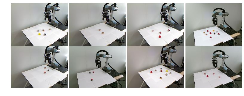
Inputs                                                                                    x
                                                                                                                     Outputs
                                                     Decoder
Joint configuration

                                                               Foreground mask
                                    Encoder                                            Object
                                                                                                     y
                                                                y                   identification
                                    ResNet                          x
                                                     Decoder

                                                                                                         Object positions      Patches

Fig. 3: The visual recognition system. The input is an image of the scene captured by an uncalibrated camera together with the joint
configuration vector of the depicted robot. Given this input a convolutional neural network (CNN) predicts the foreground-background
object segmentation mask and a dense position field that maps each pixel of the (downsampled) input image to a 2D coordinate in a
frame centered on the robot. The estimated masks and position fields are then combined by the object identification module to identify
individual object instances. The output is a set of image patches associated with the 2D position of the object in the workspace.

                                                                        IV. R EARRANGEMENT P LANNING WITH M ONTE -C ARLO
                                                                                      T REE S EARCH (MCTS)
                                                                           Given the current and target arrangements, the MCTS task
                                                                        planner has to compute a sequence of pick-and-place actions
                                                                        that transform the current arrangement into the target one.
Fig. 4: Examples of synthetic training images. We generate im-          In this section, we first review Monte-Carlo Tree Search and
ages displaying the robot and a variable number of objects in
its workspace. The images are taken by cameras with different           then explain how we adapt it for rearrangement planning.
viewpoints and depicting large scene appearance variations.
                                                                        A. Review of Monte-Carlo Tree Search
a threshold to the predicted mask yields a binary object                   The MCTS decision process is represented by a tree,
segmentation. The corresponding pixels of the 2D position               where each node is associated to a state s, and each edge
field provide a point set in the robot coordinate frame.                represents a discrete action a = {1, ..., N }. For each node in
We use the mean-shift algorithm [38] to cluster the 2D                  the tree, a reward function r(s) gives a scalar representing
points corresponding to the different objects and obtain                the level of accomplishment of the task to solve. Each node
an estimate of the position of each object. The resulting               stores the number of times it has been visited n(s) and
clusters then identify pixels belonging to each individual              a cumulative reward w(s). The goal of MCTS is to find
object providing instance segmentation of the input image.              the most optimistic path, i.e. the path that maximizes the
We use the resulting instance segmentation to extract patches           expected reward, starting from the root node and leading to
that describe the appearance of each object in the scene.               a leaf node solving the task. MCTS is an iterative algorithm
                                                                        where each iteration is composed of three stages.
                                                                           During the selection stage, an action is selected using the
C. Source-Target matching                                               Upper Confidence Bound (UCB) formula:
                                                                                                           s
   To perform rearrangement, we need to associate each                                                         2 log n(s)
                                                                                     U (s, a) = Q(s, a) + c                ,        (1)
object in the current image to an object in the target                                                         n(f (s, a))
configuration. To do so, we use the extracted image patches.
We designed a simple procedure to obtain matches robust                 where f (s, a) is the child node of s corresponding to the
to the exact position of the object within the patches, their           edge (s, a) and Q(s, a) = w(f   (s,a))
                                                                                                    n(f (s,a)) is the expected value at
background and some amount of viewpoint variations. We                  state s when choosing action a. The parameter c controls the
rescale patches to 64×64 pixels and extract conv3 features              trade-off between exploiting states with high expected value
of an AlexNet network trained for ImageNet classification.              (first term in (1)) and exploring states with low visit count
We finally run the Hungarian algorithm to find the one-to-one           (second term in (1)). We found this trade-off is crucial for
matching between source and target patches maximizing the               finding good solutions in a limited number of iterations as
sum of cosine similarities between the extracted features. We           we show in Sec. V-A. The optimistic action selected aselected
have tried using features from different layers, or from the            is the action that maximizes U (s, a) given by (1). Starting
more recent network ResNet. We found the conv3 features                 from the root node, this stage is repeated until an expandable
of AlexNet to be the most suited for the task, based on a               node (a node that has unvisited children) is visited. Then,
qualitative evaluation of matches in images coming from the             a random unvisited child node s0 is added to the tree in
dataset presented in Sec. V-B . Note that our patch matching            the expansion stage. The reward signal r(s0 ) is then back-
strategy assumes all objects are visible in the source and              propagated towards the root node in the back-propagation
target images.                                                          stage, where the cumulative rewards w and visit counts n of
                                                                        all the parent nodes are updated. The search process is run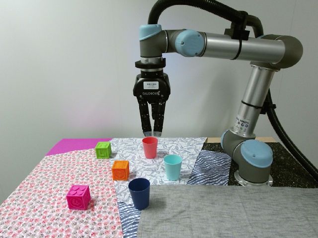
Initial Target
1
7
3 2 4
5 7
8 5 6 7 a position inside the workspace that does not overlap with
5 3
7
3
6
2
6
6
9
3
2
6
9
10
4
3 2 1
Tk (lines 8-10 in Algo. 1). The position P where to place
2
7
3
8
5 8
5
2 1 11
7
8
9 j is found using random sampling (line 8). For collision
1 1 4 3 5
4
9
4
10
11
5 2
6
5
4
checks, we consider simple object collision models with
4 1
4 1 1
2
3
fixed radiuses as depicted in Figure 5. If no suitable position
Fig. 5: Examples of source and target object configurations. The is found, no objects are moved (line 11). Note that additional
planner has to find a sequence of actions (which object to move heuristics could be added to the action parametrization to
and where to displace it inside the workspace), while avoiding further improve the quality of the resulting solutions and to
collisions with other objects. Workspace limits are shown as dashed reduce the number of iterations required. Examples include
lines. Grey circles depict the collision radius for each object. (i) avoiding to place j at target positions of other objects and
We demonstrate our method solving this complex rearrangement
problem in the supplementary video. Here source and target states
(ii) restricting the search for position P in a neighborhood of
are known (state estimation network is not used). Cj . The parameters of the pick-and-place motion for a given
state and MCTS action are computed only once during the
expansion stage and then cached in the tree and recovered
iteratively until the problem is solved or a maximal number once a solution is found.
of iterations is reached.
Algorithm 1: Action Parametrization
B. Monte-Carlo Tree Search task planner 1 function GET MOTION({Ci }i , {Ti }i , k):
2 /* Check if object k can be moved to Tk */
We limit the scope to tabletop rearrangement planning 3 if IS MOVE VALID ({Ci }i6=k , Ck , Tk ) then
problems with overhand grasps but our solution may be 4 return (Ck , Tk )
applied to other contexts. We assume that the complete state 5 else
6 /* Move obstructing object j to position P */
of any object is given by its 2D position in the workspace, 7 j = FIND CLOSEST OBJECT ({Ci }i , Tk )
and this information is sufficient to grasp it. The movements 8 found, P = FIND POSITION ({Ci }i6=j ∪ {Tk })
are constrained by the limited workspace, and actions should 9 if found then
10 return (Cj , P)
not result in collisions between objects. The planner has to
11 return (Ck , Ck )
compute a sequence of actions which transform the source
arrangement into the target arrangement while satisfying
these constraints. Each object can be moved multiple times
and we do not assume that explicit buffer space is available. As opposed to games where a complete game must be
An example of source and target configurations is depicted played before having access to the outcome (win or lose), the
in Fig. 5. We now detail the action parametrization and the reward in our problem is defined in every state. Therefore, we
reward. found that using a MCTS simulation stage is not necessary.
Let {Ci }i=1,..,N denote the list of 2D positions that define The number of MCTS iterations to build the tree is typi-
the current arrangement with N objects, {Ii }i and {Ti }i the cally a hyper-parameter. In order to have a generic method
initial and target arrangements respectively, which are fixed that works regardless of the number of objects, we adopt the
for a given rearrangement problem. MCTS state corresponds following strategy: we run MCTS until a maximum (large)
to an arrangement s = {Ci }i . number of iterations is reached or until a solution is found.
As a reward r(s) we use the number of objects located We indeed noticed that the first solution provided by MCTS
within a small distance of their target position: is already sufficiently good compared to the next ones when
N
( letting the algorithm run for longer.
X 1 if ||Ci − Ti ||2 ≤ The presented approach only considers tabletop rearrange-
r(s) = Ri with Ri = , (2)
0 otherwise. ment planning with overhand grasps. The main limitation
i=1
is that we assume the motion planning algorithm can suc-
where N is the number of objects, Ci is the current location cessfully plan all the pick-and-place motions computed in
of object i, Ti is the target location of object i and is a Algo. 1. This assumption does not hold for more complex en-
small constant. vironment where some objects are not reachable at any time
We define a discrete action space with N actions where (e.g. moving objects in a constrained space such as inside a
each action corresponds to one pick-and-place motion mov- refrigerator). In this case, the function IS MOVE VALID
ing one of the N objects. The action is hence pararametrized can be adapted to check whether the movement can be
by 2D picking and placing positions defined by the function executed on the robot. Note that we consider simple collision
GET MOTION outlined in detail in Algo. 1. The input to models in FIND POSITION but meshes of the objects and
that function is the current state {Ci }i , target state {Ti }i environment could be used if available.
and the chosen object k that should be moved. The function
proceeds as follows (please see also Algo. 1). First, if V. E XPERIMENTS
possible, the object k is moved directly to it’s target Tk We start by evaluating planning (section V-A) and visual
(lines 3-4 in Algo. 1), otherwise the obstructing object j scene state estimation (section V-B) separately, demonstrat-
which is the closest to Tk (line 7 in Algo. 1) is moved to ing that: (i) our MCTS task planner scales well with the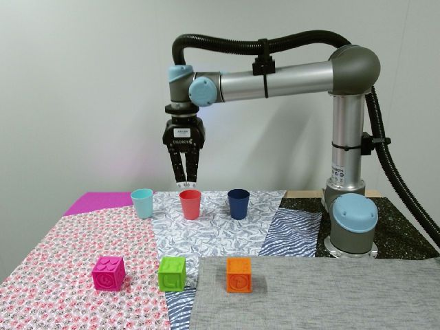
Success rate Number of object moves Number of collision checks Success rate Number of object moves Number of collision checks
number of collision checks
10^8 10^8
number of collision checks
1 1
number of object moves
80
number of object moves
mcts mcts 100
0.8 baseline baseline 0.8 mcts, c=0.0
60 10^6 mcts, c=0.5 80 10^6
success rate
success rate
y=x
0.6 0.6 mcts, c=1.0
10^4 60 10^4
40 mcts, c=3
0.4 0.4 40
mcts mcts, c=10
20 10^2 0.2 10^2
0.2 baseline baseline 20
buffer space baseline+randperm
0 0 10^0 0 0 10^0
0 10 20 30 0 10 20 30 0 10 20 30 0 10 20 30 0 10 20 30 0 10 20 30
number of objects number of objects number of objects number of objects number of objects number of objects
(a) (b) (c) (a) (b) (c)
Fig. 6: Comparison of the proposed MCTS planning approach Fig. 7: Exploration-exploitation tradeoff in MCTS. MCTS per-
against the strong baseline heuristic. MCTS is able to solve more forms better than a random baseline heuristic search. Balancing the
complex scenarios (with more objects) in a significantly lower exploration term of UCB with the parameter c is crucial for finding
number of steps. MCTS does not require free space to be available good solutions while limiting the number of collision checks.
or that the problems are monotone.
place action and perform rearrangement in a closed loop.
number of objects and is efficient enough so that it can Exploration-exploitation trade-off. We now want to
be used online (i.e. able to recompute a plan after each demonstrate that the benefits of our planning method are
movement); (ii) the visual system detects and localizes the due to the quality of the exploration/exploitation trade-off in
objects with an accuracy sufficient for grasping. Finally, in MCTS. An important metric is the total number of collision
section V-C we evaluate our full pipeline in challenging checks that the method requires for finding a plan. The
setups and demonstrate that it can efficiently perform the collision check (checking whether an object can be placed
task and can recover from errors and perturbations as also to a certain location) is indeed one of the most costly
shown in the supplementary video. operation when planning. Fig. 6(c) shows that MCTS uses
more collision checks compared to the baseline because
A. MCTS planning MCTS explores many possible optimistic action sequences
Experimental setup. To evaluate planning capabilities and while the baseline is only able to find a solution and does not
efficiency we randomly sample 3700 initial and target config- optimize any objective. We propose another method that we
urations for 1 up to 37 objects in the workspace. It is difficult refer to as baseline+randperm which solves the problem with
to go beyond 37 objects as it becomes hard to find valid the baseline augmented with a random search over action
configurations for more due to the workspace constraints. sequences: the baseline is run with different random object
Planning performance. We first want to demonstrate the orders until a number of collision checks similar to MCTS
interest of MCTS-based exploration compared to a simpler with c = 1 is reached and we keep the solution which
solution in term of efficiency and performances. As a base- has the smallest number of object moves. As can be see
line, we propose a fast heuristic search method, which simply in Fig. 7, baseline+randperm has a higher success rate and
iterates over all actions once in a random order, trying to produces higher quality plans with lower number of object
complete the rearrangement using the same action space as moves compared to the baseline (Fig. 7(b)). However, MCTS
our MCTS approach, until completion or a time limit is with c = 1, still produces higher quality plans given the
reached. Instead of moving only the closest object that is same amount of collision checks. The reason is that base-
obstructing a target position Tk , we move all the objects that line+randperm only relies on a random exploration of action
overlap with Tk to their target positions or to a free position sequences while MCTS allows to balance the exploration
inside the workspace that do not overlap with Tk . Our MCTS of new actions with the exploitation of promising already
approach is compared with this strong baseline heuristic in sampled partial sequences through the exploration term of
Fig. 6. Unless specified otherwise, we use c = 1 for MCTS UCB (equation 1). In Fig. 7, we also study the impact of the
and set the maximum number of MCTS iterations to 100000. exploration parameter c. MCTS with no exploration (c = 0)
As shown in Fig. 6(a), the baseline is able to solve finds plans using fewer collision checks compared to c > 0
complex instances but its success rate starts dropping after but the plans have high number of object moves. Increasing c
33 objects whereas MCTS is able to find plans for 37 objects leads to higher quality plans while also increasing the number
with 80% success. More importantly, as shown in Fig. 6(b), of collision checks. Setting c too high also decreases the
the number of object movements in the plans found by success rate (c=3, c=10 in Fig 7(a)) because too many nodes
MCTS is significantly lower. For example, rearranging 30 are added to the tree and the limit on the number of MCTS
objects takes only 40 object moves with MCTS compared iterations is reached before finding a solution.
to 60 with the baseline. This difference corresponds to more Generality of our set-up. Previous work for finding high-
than 4 minutes of real operation in our robotics setup. The quality solutions to rearrangement problems has been limited
baseline and MCTS have the same action parametrization to either monotone instances [13] or instances where buffer
but MCTS produces higher quality plans because it is able space is available [10]. The red curve in Fig. 6(a) clearly
to take into consideration the future effects of picking-up an shows that in our set-up the number of problems where
object and placing it at a specific location. On a laptop with a some buffer space is available for at least one object quickly
single CPU core, MCTS finds plans for 25 objects in 60 ms. decreases with the number of objects in the workspace. In
This high efficiency allows to replan after each pick-and- other words, the red curve is an upper bound on the success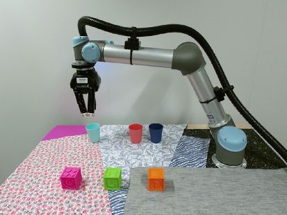
Success rate Number of object moves Number of collision checks Error below threshold (%) Object identification success (%)
1
number of collision checks
number of object moves
20
STRIPStream 10^5
0.8
HPP 15 10^4
success rate
0.6 mRS
plRS 10 10^3
0.4
PRM(mRS) 10^2 2.0 cm
0.2 PRM(plRS) 5
10^1 3.0 cm
mcts grasp.
0
2 4 6 8 10 2 4 6 8 10 2 4 6 8 10
number of objects number of objects
number of objects number of objects number of objects (a) (b)
(a) (b) (c)
Fig. 9: (a) Example images from the dataset that we use to evaluate
Fig. 8: Comparison of our MCTS planning approach with several the accuracy of object position estimation as a function of number of
other state-of-the-art methods. MCTS performs better than other objects. (b) Evaluation of our visual system for a variable number of
methods applied to the rearrangement planning problem. MCTS objects. We report the localization accuracy (left) and the percentage
finds high quality plans (b) using few collisions checks (c) with of images where all objects are correctly identified (right). Please
100% success rate for up to 10 objects. see the supplementary video for examples where our system is used
in more challenging visual conditions.
rate of [10], which requires available buffer space. In order of collision checks (Fig. 8(c)). Overall, the main limitation
to evaluate the performance of our approach on monotone of STRIPSTream, PRM(mRS) and PRM(plRS) comes from
problems, we generated the same number of problems but the fact that the graph of possible states is sampled randomly
the target configuration was designed by moving object whereas MCTS will prioritize the most optimistic branches
from the initial configuration one by one, in a random (exploitation). MCTS and it’s tree structure also allows to
order into free space. This ensures that the instances are build the action sequence progressively (moving one object
monotone and can be solved by moving each object once. at once) compared to PRM-based approaches that sample
Our MCTS-based approach was able to solve 100% of these entire arrangements and then try to solve them.
instances optimally in N steps. Our method can therefore
solve the problems considered in [13] while also being B. Visual scene state estimation
able to handle significantly more challenging non-monotonic Experimental setup. To evaluate our approach, we created a
instances, where objects need to be moved multiple times. dataset of real images with known object configurations. We
Comparisons with other methods. To demonstrate that used 1 to 12 small 3.5 cm cubes, 50 configurations for each
other planning methods do not scale well when used in number of cubes, and captured images using two cameras
a challenging scenario similar to ours, we compared our for each configuration, leading to a total of 1200 images
planner with three other methods of the state of the art: depicting 600 different configurations. Example images from
STRIPStream [12], the Humanoid Path-Planner [14], mRS this evaluation set are shown in Fig. 9(a).
and plRS [8]. Results are presented in Fig. 8 for 900 Single object accuracy. When a single object is present in
random rearrangement instances, we limit the experiments to the image, the mean-shift algorithm always succeeds and the
problems with up to 10 objects as evaluating these methods precision of our object position prediction is 1.1 ± 0.6 cm.
for more complex problems is difficult given a reasonable This is comparable to the results reported in [33] for posi-
amount of time (few hours). HPP [14] is the slowest method tioning of a known object with respect to a known table
and could not handle more than 4 objects, taking more without occlusions and distractors, 1.3 ± 0.6 cm, and to
than 45 minutes of computation for solving the task with results reported in [32] for the coarse alignment of a single
4 objects. HPP fails to scale because it attempts to solve the object with respect to a robot, 1.7 ± 3.4 cm. The strength of
combined task and motion planning problem at once using our method, however, is that this accuracy remains constant
RRT without explicit task/motion planning hierarchy thus for up to 10 previously unknown objects, a situation that
computing many unnecessary robot/environment collision neither [33] nor [32] can deal with.
checks. The other methods adopt a task/motion planning Accuracy for multiple objects. In Fig. 9(b), we report
hierarchy and we compare results for the task planners only. the performance of the object localization and object iden-
The state-of-the-art task and motion planner for general tification modules as a function of the number of objects.
problems, STRIPSStream [12], is able to solve problems with For localization, we report the percentage of objects local-
up to 8 objects in few seconds but do not scale (Fig. 8(a)) ized with errors below 2 cm and 3 cm respectively. For 10
when target locations are specified for all objects in the objects, the accuracy is 1.1 ± 0.6 cm. The 3 cm accuracy
scene as it is the case for rearrangement planning problems. approximately corresponds to the success of grasping, that
The success rate of specialized rearrangement methods, mRS we evaluate using a simple geometric model of the gripper.
and plRS, drops when increasing number of objects because Note that grasping success rates are close to 100% for up
these methods cannot handle situations where objects are to 10 objects. As the number of objects increases, the object
permuted, i.e. placing an object at its target position requires identification accuracy decreases slightly because the objects
moving another objects first thus requiring longer term start to occlude one each other in the image. This situation
planning capability. When used in combination with a PRM, is very challenging when the objects are unknown because
more problems can be addressed but the main drawback is two objects that are too close can be perceived as a single
that these methods are slow as they perform a high number larger object. Note that we are not aware of another method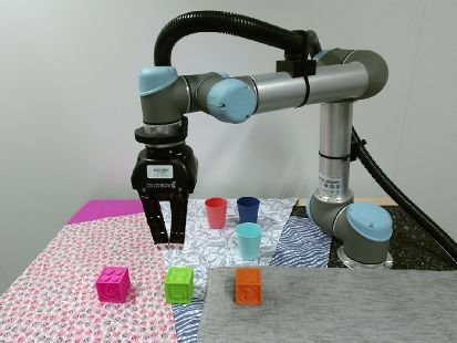
that would be able to directly predict the workspace position      on table-top re-arrangement, the proposed MCTS approach
of multiple unseen objects with unknown dimensions using           is general and opens-up the possibility for efficient re-
only (uncalibrated) RGB images as input.                           arrangement planning in 3D or non-prehensile set-ups.
Discussion. Our experiments demonstrate that our visual
predictor is able to scale well up to 10 objects with a                                         R EFERENCES
constant precision that is sufficient for grasping. We have
                                                                    [1] R. Alami, T. Simeon, and J.-P. Laumond, “A geometrical approach
also observed that our method is able to generalize to objects          to planning manipulation tasks. the case of discrete placements and
with shapes not seen during training, such as cups or plastic           grasps,” in Symposium on Robotics research, 1990.
toys. While we apply our visual predictor to visually guided        [2] T. Siméon, J.-P. Laumond, J. Cortés, and A. Sahbani, “Manipulation
                                                                        planning with probabilistic roadmaps,” The International Journal of
rearrangement planning, it could be easily extended to other            Robotics Research.
contexts using additional task-specific synthetic training data.    [3] S. M. LaValle, Planning algorithms, 2006.
Accuracy could be further improved using a refinement               [4] M. Stilman, J.-U. Schamburek, J. Kuffner, and T. Asfour, “Manipula-
similar to [32]. Our approach is limited to 2D predictions              tion planning among movable obstacles,” in ICRA, 2007.
                                                                    [5] J.-C. Latombe, Robot motion planning, 2012.
for table-top rearrangement planning. Predicting 6DoF pose          [6] L. P. Kaelbling and T. Lozano-Pérez, “Hierarchical task and motion
of unseen objects precise enough for robotic manipulation               planning in the now.” 2011.
remains an open problem.                                            [7] G. Havur et al., “Geometric rearrangement of multiple movable objects
                                                                        on cluttered surfaces: A hybrid reasoning approach,” in ICRA, 2014.
                                                                    [8] A. Krontiris and K. E. Bekris, “Dealing with difficult instances of
C. Real robot experiments using full pipeline                           object rearrangement.” in RSS, 2015.
   We evaluated our full pipeline, performing both online           [9] N. T. Dantam, Z. K. Kingston, S. Chaudhuri, and L. E. Kavraki,
                                                                        “Incremental task and motion planning: A constraint-based approach.”
visual scene estimation and rearrangement planning by per-              in Robotics: Science and systems, vol. 12. Ann Arbor, MI, USA,
forming 20 rearrangement tasks, each of them composed                   2016, p. 00052.
with 10 objects. In each case, the target configuration was        [10] H. Shuai, N. Stiffler, A. Krontiris, K. E. Bekris, and J. Yu, “High-
described by an image of a configuration captured from                  quality tabletop rearrangement with overhand grasps: Hardness results
                                                                        and fast methods,” in Robotics: Science and Systems (RSS), Cam-
a different viewpoint, with a different table texture and               bridge, MA, 07/2017 2017.
a different type of camera. Despite the very challenging           [11] S. Srivastava, E. Fang, L. Riano, R. Chitnis, S. Russell, and P. Abbeel,
nature of the task, our system succeeded in correctly solving           “Combined task and motion planning through an extensible planner-
                                                                        independent interface layer,” in ICRA, 2014.
17/20 of the experiments. In case of success, our system           [12] C. R. Garrett, T. Lozano-Pérez, and L. P. Kaelbling, “PDDLStream:
used on average 12.2 steps. The three failures were due to              Integrating symbolic planners and blackbox samplers via optimistic
errors in the visual recognition system (incorrectly estimated          adaptive planning,” 2020.
                                                                   [13] A. Krontiris and K. E. Bekris, “Efficiently solving general rearrange-
number of objects, mismatch of source and target objects).              ment tasks: A fast extension primitive for an incremental sampling-
Interestingly, the successful cases were not always perfect             based planner,” in ICRA, 2016.
runs, in the sense that the re-arrangement strategy was not        [14] J. Mirabel, S. Tonneau, P. Fernbach, A. Seppälä, M. Campana,
                                                                        N. Mansard, and F. Lamiraux, “HPP: A new software for constrained
optimal or that the visual estimation confused two objects              motion planning,” in IROS, 2016.
at one step of the matching process. However, our system           [15] M. Toussaint, “Logic-geometric programming: An optimization-based
was able to recover robustly from these failures because                approach to combined task and motion planning,” in Twenty-Fourth
                                                                        International Joint Conference on Artificial Intelligence, 2015.
it is applied in a closed-loop fashion, where then plan is         [16] R. Munos et al., “From bandits to monte-carlo tree search: The op-
recomputed at each object move.                                         timistic principle applied to optimization and planning,” Foundations
   The supplementary video shows additional experi-                     and Trends R in Machine Learning, vol. 7, no. 1, pp. 1–129, 2014.
ments including objects other than cubes, different back-          [17] S. Garrido-Jurado et al., “Automatic generation and detection of highly
                                                                        reliable fiducial markers under occlusion,” Pattern Recognit., 2014.
grounds, a moving hand-held camera and external perturba-          [18] Y. Li, G. Wang, X. Ji, Y. Xiang, and D. Fox, “Deepim: Deep iterative
tions, where an object is moved during the rearrangement.               matching for 6d pose estimation,” in Proceedings of the European
These results demonstrate the robustness of our system. To              Conference on Computer Vision (ECCV), 2018, pp. 683–698.
                                                                   [19] Y. Xiang, T. Schmidt, V. Narayanan, and D. Fox, “Posecnn: A
the best of our knowledge, rearranging a priory unknown                 convolutional neural network for 6d object pose estimation in cluttered
number of unseen objects with a robotic arm while relying               scenes,” in RSS, 2018.
only on images captured by a moving hand-held camera and           [20] J. Tremblay et al., “Deep object pose estimation for semantic robotic
                                                                        grasping of household objects,” in CoRL, 2018.
dealing with object perturbations has not been demonstrated        [21] G. Wilfong, “Motion planning in the presence of movable obstacles,”
in prior work.                                                          Annals of Mathematics and Artificial Intelligence, 1991.
                       VI. C ONCLUSION                             [22] S. Russel and P. Norvig, “Artificial intelligence: A modern approach,”
                                                                        2003.
   We have introduced a robust and efficient system for            [23] P. E. Hart, N. J. Nilsson, and B. Raphael, “A formal basis for the
online rearrangement planning, that scales to many objects              heuristic determination of minimum cost paths,” IEEE Transactions
and recovers from perturbations, without requiring calibrated           on Systems Science and Cybernetics, 1968.
camera or fiducial markers on objects. To our best knowl-          [24] C. Paxton, V. Raman, G. D. Hager, and M. Kobilarov, “Combining
                                                                        neural networks and tree search for task and motion planning in
edge, such a system has not been shown in previous work.                challenging environments,” in IROS, 2017.
At the core of our approach is the idea of applying MCTS           [25] M. Toussaint and M. Lopes, “Multi-bound tree search for logic-
to rearrangement planning, which leads to better plans,                 geometric programming in cooperative manipulation domains,” in
                                                                        ICRA, 2017.
significant speed-ups and ability to address more general set-     [26] D. Silver and A. H. et al., “Mastering the game of go with deep neural
ups compared to prior work. While in this work we focus                 networks and tree search,” Nature, 2016.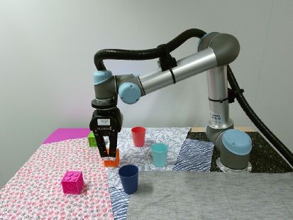
[27] J. Wu, B. Zhou, R. Russell, V. Kee, S. Wagner, M. Hebert, A. Torralba,
     and D. M. S. Johnson, “Real-time object pose estimation with pose
     interpreter networks,” in IROS, 2018.
[28] A. Zeng, K.-T. Yu, S. Song, D. Suo, E. Walker Jr, A. Rodriguez,
     and J. Xiao, “Multi-view self-supervised deep learning for 6D pose
     estimation in the amazon picking challenge,” in ICRA, 2016.
[29] T. Hodaň, J. Matas, and Š. Obdržálek, “On evaluation of 6D object
     pose estimation,” in ECCV Workshops, 2016.
[30] R. Horaud and F. Dornaika, “Hand-eye calibration,” The international
     journal of robotics research, vol. 14, no. 3, pp. 195–210, 1995.
[31] J. Heller et al., “Structure-from-motion based hand-eye calibration
     using L-∞ minimization,” in CVPR, 2011.
[32] V. Loing, R. Marlet, and M. Aubry, “Virtual training for a real appli-
     cation: Accurate object-robot relative localization without calibration,”
     IJCV, 2018.
[33] J. Tobin et al., “Domain randomization for transferring deep neural
     networks from simulation to the real world,” IROS, 2017.
[34] F. Sadeghi, A. Toshev, E. Jang, and S. Levine, “Sim2real viewpoint
     invariant visual servoing by recurrent control,” in CVPR 2018, 2018,
     p. 8.
[35] S. James and P. e. a. Wohlhart, “Sim-to-Real via Sim-to-Sim: Data-
     efficient robotic grasping via Randomized-to-Canonical adaptation
     networks,” CVPR, 2019.
[36] K. He, X. Zhang, S. Ren, and J. Sun, “Deep residual learning for
     image recognition,” CVPR, 2016.
[37] D. P. Kingma and J. Ba, “Adam: A method for stochastic optimiza-
     tion,” in 3rd International Conference on Learning Representations,
     ICLR 2015, San Diego, CA, USA, May 7-9, 2015, Conference Track
     Proceedings, 2015.
[38] D. Comaniciu and P. Meer, “Mean shift: A robust approach toward
     feature space analysis,” IEEE Trans. Pattern Anal. Mach. Intell., 2002.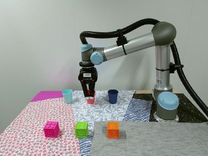
You can also read