The elasticity of taxable income - New data and estimates for South Africa WIDER Working Paper 2020/29 - unu-wider
←
→
Page content transcription
If your browser does not render page correctly, please read the page content below

WIDER Working Paper 2020/29

The elasticity of taxable income

New data and estimates for South Africa

Johannes Hermanus Kemp*

March 2020
Abstract: The elasticity of taxable income is a key tax policy parameter that plays an important
role in the formulation of tax and transfer policy. This paper extends work by Kemp (2019) by
using a new panel of individual tax returns and the phenomenon of ‘bracket creep’ to produce
updated estimates of the elasticity of taxable income for South Africa. Whereas the previous
work focused on assessed taxpayers (i.e. individual assessed tax returns), the current study uses a
newly constructed panel for the period 2010–16 that includes information captured on both
individual income tax return (ITR12) and employee tax certificate (IRP5) forms. The elasticity of
taxable income is estimated at around 0.4, somewhat higher than the estimate presented
previously. The elasticity for broad income is estimated at around 0.2, similar in size to the earlier
study. As in that earlier study, it was found that behavioural responses are concentrated in
higher-income groups, as suggested by the higher elasticity estimates for individuals in the top
two income tax brackets and the top 10 per cent of income earners. An important finding is that
the ETI for high-income earners increases notably in the latter half of the sample, mainly due to
increased itemized deductions in the face of a rising tax burden due to insufficient bracket
adjustments and rising marginal rates.
Key words: fiscal policy, elasticity, taxable income, optimal tax
JEL classification: H21, H31, J22

* Bureau for Economic Research, Stellenbosch University, Stellenbosch, South Africa; johannes.kemp@gmail.com
This study has been prepared within the UNU-WIDER project Southern Africa – Towards Inclusive Economic Development
(SA-TIED).
Copyright © UNU-WIDER 2020
Information and requests: publications@wider.unu.edu
ISSN 1798-7237 ISBN 978-92-9256-786-6
https://doi.org/10.35188/UNU-WIDER/2020/786-6
Typescript prepared by Gary Smith.
The United Nations University World Institute for Development Economics Research provides economic analysis and policy
advice with the aim of promoting sustainable and equitable development. The Institute began operations in 1985 in Helsinki,
Finland, as the first research and training centre of the United Nations University. Today it is a unique blend of think tank,
research institute, and UN agency—providing a range of services from policy advice to governments as well as freely available
original research.
The Institute is funded through income from an endowment fund with additional contributions to its work programme from
Finland, Sweden, and the United Kingdom as well as earmarked contributions for specific projects from a variety of donors.
Katajanokanlaituri 6 B, 00160 Helsinki, Finland
The views expressed in this paper are those of the author(s), and do not necessarily reflect the views of the Institute or the
United Nations University, nor the programme/project donors.
1          Introduction

The size of the behavioural response of taxpayers to changing tax rates is central to the formulation
of tax and transfer policies, as well as the study of the welfare implications of tax decisions. In this
regard, the elasticity of taxable income (ETI) is a key concept. The ETI captures all possible responses
to changing tax rates in a single measure (Creedy 2009; Thoresen and Vattø 2013).1

As mentioned by Saez et al. (2012), a large body of literature has sought to estimate the ETI and elas-
ticities for related income measures. Most of the literature has focused on the United States, Canada,
and Western Europe, but a limited number of studies have focused on countries and regions outside
these developed economies. Feldstein (1995) pioneered the use of panel data to estimate the ETI for the
United States around the Tax Reform Act of 1986, generating large ETI estimates ranging from one to
three in alternative specifications. Using Feldstein’s (1995) approach, Moffitt and Wilhelm (2000) found
elasticities around the 1986 tax reform ranging from 1.76 to 1.99.

Subsequent researchers have used innovative research designs to overcome the two main identification
issues highlighted in the literature, namely mean reversion and secular changes in the income distri-
bution. Mean reversion refers to the phenomenon that high incomes in one year tend to be lower in
following years, and vice versa for low incomes in year 1. ETI estimates might also be biased because
of the presence of changes in the (taxable) income distribution unrelated to changes in the tax structure.
Auten and Carroll (1999) addressed mean reversion and attempted to control for the divergence in the
income distribution by including base year income controls, as well as controls for region and occupa-
tion. Including these controls leads to much lower ETI estimates in the region of 0.5 for taxable income.
Subsequent research included even richer income controls in order to control for mean reversion and/or
changing income distribution in a more robust fashion.2

Very little work has been done in the South African context. Tax research in South Africa has focused
on the impact of specific tax measures and the welfare implications of the broader tax system. Examples
include research on the impact of the employment tax incentive, the impact of introducing a nega-
tive income tax, welfare implications of specific tax allowances/deductions, the impact and incidence
of value-added tax (VAT), and numerous studies investigating different aspects of corporate taxation.3
However, very little work has been done in the South African context with respect to the estimation of
the ETI. One exception is Van Heerden (2013), who estimated implied personal income tax elasticities
of between 0.38 and 0.79 for the various income groups under consideration. Kemp (2019) uses the
phenomenon of ‘bracket creep’ and finds an overall ETI equal to approximately 0.3.

Using a new dataset comprising confidential tax return data made available for research purposes by
the South African Revenue Service (SARS) and the National Treasury, this paper provides updated ETI
estimates for South Africa. Much of the international literature uses tax reforms to identify the ETI.
However, considering the fact that there was no large legislated tax reforms in South Africa over the
sample period, Saez (2003) and Kemp (2019) are followed in using the phenomenon of ‘bracket creep’
to identify the ETI.

1 These behavioural responses include adjustment to labour supply, tax evasion and/or avoidance, and income and/or profit
shifting, among others.
2 See Moffitt and Wilhelm (2000), Gruber and Saez (2002), Saez (2003, 2010), Kopczuk (2005), Giertz (2007), Auten et
al. (2008), Singleton (2011), and Weber (2014) for examples. See Piketty (1999), Sillamaa and Veall (2001), Selén (2002),
Gottfried and Schellhorn (2004), Saez and Veall (2005), Pirttilä and Selin (2006), Hansson (2007), Atkinson and Leigh (2008),
Saez et al. (2009), Gorodnichenko et al. (2009), Brewer et al. (2010), Chetty et al. (2011), Kopczuk et al. (2012), and Kleven
and Schultz (2014) for ETI studies focusing on regions outside the United States.
3   See Ebrahim et al. (2019) for a review of tax research in South Africa.

                                                                 1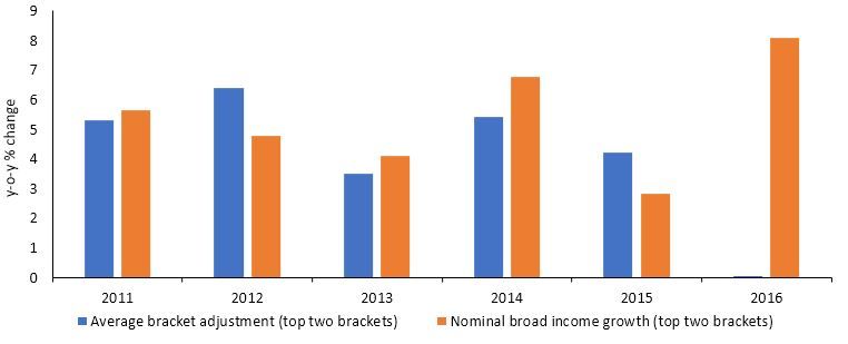
As is clear from the international literature, there is no reason to believe that the ETI will be constant over
time or uniform across regions/countries. The ETI depends crucially on the nature of the tax structure
and other institutional arrangements, which are not constant over time or across countries. This is borne
out by the fact that the updated ETI estimates presented in this paper differ somewhat from those in
Kemp (2019), who used a different sample. The overall ETI for the current sample is estimated at
around 0.4, while that for broad income is estimated at closer to 0.2. As in Kemp (2019), it was found
that behavioural responses are concentrated in higher-income earners, as suggested by the much higher
elasticity estimate of 0.5 for taxable income for the top 10 per cent of income earners.

The rest of the paper proceeds as follows: Section 2 estimates the ETI for South Africa using micro-level
tax return data and conducts a sensitivity analysis. Section 3 compares the updated estimates to those
from earlier studies, while Section 4 presents some caveats and concludes the paper.

2        Updated ETI estimates for South Africa

2.1      Identification of the ETI using ‘bracket creep’

Kemp (2019) highlights the fact that a lack of the type of major tax reforms that are usually used to
identify the ETI complicates identification. There was no large, policy-induced variation in marginal tax
rates—of the kind that is often used to identify and estimate the ETI—introduced over either the sample
period in the earlier study (2008/09 to 2012/13) or the current sample period (2010/11 to 2016/17). As
such, I follow the same method as in Kemp (2019) (based on Saez (2003))—that is, the phenomenon of
‘bracket creep’, to identify and estimate the ETI, extending the sample to include a broader definition of
taxpayer.4

The National Treasury often adjusts individual tax brackets to compensate for the effects of inflation.
Without these adjustment, taxpayers might graduate to a higher tax bracket despite the fact that their
real taxable income did not change. The degree of the adjustment depends crucially on the policy and
revenue requirements at the time of the adjustment. For example, if central revenues are under pressure
(as has been the case over recent years), the adjustments might be smaller. The expectation is that this
would lead to an automatic increase in tax revenue as taxpayers graduate to higher brackets.

The extent to which official bracket adjustments compensate for inflation depends critically on the mea-
sure of inflation under consideration. Official inflation measures (such as the CPI or GDP deflator) might
underestimate the extent to which nominal incomes change from year to year. If nominal wages increase
in excess of official inflation measures, then taxpayers near the top end of an income tax bracket will be
pushed into the next bracket (Kemp 2019).

As an illustration, Table 1 shows the average effective bracket adjustment for each tax year, together with
two widely used inflation measures and a measure of economy-wide wage inflation, over the sample
period. While bracket adjustments were generally larger than inflation as measured by the CPI and GDP
deflator in 2011/12 and 2012/13, adjustments in subsequent years did not keep pace with official inflation
measures. In fact, average adjustments were significantly below inflation in 2015/16 and 2016/17, with
adjustment for higher brackets even lower than the averages displayed in the table.

That being said, the relevant inflation measure when studying the effects of ‘bracket creep’ is nominal
wage inflation. When comparing average bracket adjustments to economy-wide wage inflation, it is clear

4 A new top tax bracket was introduced in the 2018/19 tax year. This policy-induced variation could be used in the future to
estimate the ETI for high-income earners.

                                                             2
Table 1: Bracket adjustment and inflation
Tax year Average bracket CPI inflation GDP deflator Economy-wide
adjustment (%) (%) (%) wage rate (%)
2011/12 6.1 5.6 6.1 10.2
2012/13 6.5 5.5 5.6 8.7
2013/14 3.5 5.8 5.9 9.8
2014/15 5.4 5.6 5.2 8.6
2015/16 4.2 5.2 6.3 8.2
2016/17 2.0 6.3 6.2 8.0
Notes: inflation rates calculated as year-on-year percentage changes in CPI, the GDP deflator, and the total economy-wide
wage rate.
Source: author’s compilation, based on data from the National Treasury, the South African Revenue Service, Statistics South
Africa, and the South African Reserve Bank.
that official bracket adjustments were generally much lower than nominal wage inflation. This suggests
that a significant proportion of taxpayers likely migrated to higher tax brackets (especially in the latter
years of the sample) and faced a higher marginal tax rate in the following tax year as a consequence. As
in Kemp (2019), in the absence of significant reforms, it is this phenomenon of ‘bracket creep’ that is
used to identify the ETI.
As mentioned in Kemp (2019), this identification strategy has one major drawback: given the fact that
‘bracket creep’ is not a publicized, legislated tax reform of the sort that is normally used in the identifi-
cation process, and that it likely affects taxpayers only on the margin, the average taxpayer might not be
fully aware of the small change to the tax code and, as such, any estimated behavioural response will be
muted. Indeed, there was relatively little variation in marginal tax rates between 2011/12 and 2016/17.
As in Kemp (2019), this implies that the estimated ETI likely underestimates the true behavioural re-
sponse to changing tax rate.
2.2 Data and descriptive statistics
The analysis presented here uses confidential tax return data, made available for research purposes by
SARS and the National Treasury. The available sample runs from 2010 to 2016.5 As in Kemp (2019),
the full dataset contains most items found on individual employee tax certificate (IRP5) and income tax
return (ITR12) forms. This includes information on various aspects of personal income taxation, includ-
ing gross and taxable income, deductions, exemptions and allowances, and total tax liability. Whereas
Kemp (2019) focused only on those taxpayers who submitted tax returns that were, in turn, assessed by
SARS, the current study extends the analysis to include information from employee tax certificates (i.e.
IRP5 forms).
To that end, I use a panel constructed by Ebrahim and Axelson (2019). The authors construct an
anonymized individual panel from the combination of payroll and personal income tax records. The in-
dividual panel expanded on the available administrative data in the matched employer–employee panel,
the Company Income Tax-RP5 (CIT-IRP5) panel, as described in Pieterse et al. (2018). Ebrahim and
Axelson (2019) expanded the CIT-IRP5 panel to include information from ITR12 returns. The latter
provides additional income information such as information on self-employment income, rental income,
and retirement annuity contributions. By combining the ITR12 and IRP5/IT3(a)6 tax records, the indi-
vidual panel creates a more complete picture of the income distribution, as well as providing detailed
5 The sample runs from the 2010/11 tax year to the 2016/17 tax year. For notational convenience, the paper will refer only to
the calendar year that comprises the largest proportion of the relevant tax year—for example, 2010/11 becomes 2010, 2011/12
becomes 2011.
6 An IT3(a) is the same as an IRP5 except that it shows employee earnings from which tax has not been deducted.
3information on the sources of income, deductions and exemptions, and information on the associated
tax liability.
Using the above-mentioned dataset, a balanced panel was constructed by selecting only those individ-
uals present in each of the years in the sample, resulting in just over seven million observations per
year.7 Table 2 presents means and standard deviations of the relevant income data (in real terms) for the
constructed panel over the entire sample period (2010–16).
Table 2: Summary statistics: balanced panel (2010–16; constant 2010 prices)
Mean Std dev.
Broad income R160,259 R320,582
Exemptions R6,113 R35,573
Deductions R22,713 R36,850
Taxable income R142,188 R295,503
Tax liability R25,928 R109,521
Itemizers 52%
Number of observations 49,047,999
Notes: statistics for exemptions and deductions were calculated by only taking into account those individuals with recorded
values for the respective items.
Source: author’s compilation, based on data from the National Treasury.
As in previous studies, two income definitions are used: gross or broad income, and taxable income.
Broad income is an extensive definition of income that is consistent across all the years in the sample
(Kemp 2019). It includes most of the items that are summed to arrive at total income: wage income,
investment income, business income, fringe benefits, allowances, and so on. Taxable income is defined
as broad income less exemptions and other allowable deductions.8
According to Table 2, average (real) broad income in the sample equalled about R160,000 and average
(real) taxable income equalled around R142,000. Approximately 52 per cent of the individuals in the
dataset recorded itemized deductions. These values are significantly lower than those recorded by Kemp
(2019), even when comparing nominal values. One reason is that Kemp (2019) only considered assessed
income tax returns. Between 2007 and 2011, individual taxpayers in South Africa were not liable to file a
tax return if their employment income was less than R120,000 per annum, provided that the income was
derived from employment only. This limit was increased to R250,000 in 2012, to R350,000 in 2015, and
to R500,000 in 2019. This implies that only higher-income individuals, and those with significant scope
for claiming exemptions and/or deductions, would file income tax returns. Therefore, average income
levels would be significantly higher when focusing only on assessed income tax return data. Including
information for those taxpayers who did not file returns (i.e. directly from IRP5 forms) implies that
average income levels would naturally be lower. In the same vein, the share of itemizers is smaller in
the current sample as it is only those individuals who file income tax returns that qualify for meaningful
exemptions and/or deductions.
As mentioned above, our inflation measure is based on the average growth of broad income for each of
the years in the sample. Taking 2010 as the base year index (equal to 100), the incomes for years 2011
to 2016 have been deflated using the following indices: 112.74, 124.75, 137.26, 151.52, 162.66, and
186.78.
7 Before creating the panel, the dataset was cleaned by removing several outliers, selecting only on those individuals with
recorded values for gross and taxable income, and selecting only those individuals between the ages of 16 and 99. No trans-
formations were applied.
8 See Ebrahim and Axelson (2019) for details on the constructions of the income variables.
42.3 Empirical strategy
Following Gruber and Saez (2002) and Kemp (2019), the empirical strategy is to relate changes in
income between pairs of years to the change in marginal tax rates between the same pairs of years. The
time length between year 1 (the base year) and year 2 is set at three years. Therefore, year 2013 is
related to year 2010, and year 2014 to year 2011, etc. These four differences are stacked to obtain a
single dataset of about 28 million observations. Given the fact that the identification strategy employed
here relies on what is essentially unobserved tax rate changes, the three-year time lag allows for a more
complete behavioural response as taxpayers become aware of the tax implications of ‘bracket creep’
(Kemp 2019).
The basic model discussed in Kemp (2019) is used to derive a regression specification. This boils down
to estimating ec in Equation (1):9
dz dτ dR − zdτ
= −ec +η (1)
z 1−τ z(1 − τ )
where z is real income, ec is the compensated ETI, τ is the marginal tax rate, η gives the income effect,
and R is virtual income. Following Gruber and Saez (2002) and Kemp (2019), this equation can be
estimated by replacing z by z1 (year 1 income), dz by z2 − z1 (change in income between year 1 and year
2), dτ by T20 (z2 ) − T10 (z1 ) (the change in marginal tax rates), and dR − z by [z2 − T2 (z2 )] − [z1 − T1 (z1 )]
(the change in after-tax income).
Using the log-log specification and replacing dz/z by log(z2 /z1 ), −dτ /(1 − τ ) by log[(1 − T20 )/(1 − T10 )],
and (dR − zdτ )(z(1 − τ )) by log[(z2 − T2 (z2 ))/(z1 − T1 (z1 ))], the following regression specification is
obtained:
log(z2 /z1 ) = e log[(1 − T20 )/(1 − T10 )] + η log[(z2 − T2 (z2 ))/(z1 − T1 (z1 ))] + ε (2)
where e is the compensated elasticity parameter, η is the income effect parameter, zi is real income in
year i, Ti0 is the marginal tax rate in year i, and Ti (zi ) is the tax liability in year i.
This framework serves to highlight the main identification problem found in the literature. The term
capturing the change in the marginal tax rate, log[(1 − T20 )/(1 − T10 )], is correlated with the error term
ε because a positive shock to income could generate an automatic increase in the marginal rate due
to the progressive nature of the income tax system. As in Kemp (2019), an instrument is constructed
by computing Tp0 , the marginal tax rate that an individual would face in year 2 if their real income
did not change from year 1 to year 2. A natural instrument for log[(1 − T20 )/(1 − T10 )] is therefore
log[(1 − Tp0 )/(1 − T10 )], or the predicted change in the log net-of-tax rate if real income does not change
between year 1 and year 2.
According to Gruber and Saez (2002), running an instrumental variables (IV) regression of Equation
(2) might still lead to a biased estimate of the elasticity if ε is correlated with z1 . This relates to the
phenomenon of mean reversion and a changing income distribution (see Kemp (2019) for details). As
such, many studies in the literature follow Auten and Carroll (1999) in including several controls (no-
tably controlling for some functions of lagged income) in order to control for mean reversion and/or a
changing income distribution.
Turning to the income effect, the term log[(z2 − T2 (z2 ))/(z1 − T1 (z1 ))] will also be correlated with ε
for the same reasons discussed above, leading to biased estimates for the income effect parameter η.
However, in much of the literature, the income effect is assumed away (i.e. η = 0) since those studies
9 See Kemp (2019) for a full discussion on the basic theoretical model.
5that do estimate income effects often find them to be small and insignificant. As in Kemp (2019), there
is an additional motivation for omitting income effects from the base specification. In the presence of
‘bracket creep’, the income effect term affects those individuals who experience a change in marginal
rates (treatments) and those individuals who do not experience a change in marginal rates (controls) in
approximately the same way. Therefore, this additional income effect can be incorporated into the error
term.10
That being said, it is theoretically feasible to estimate income effects in the current set-up. A natural
instrument for log[(z2 −T2 (z2 ))/(z1 −T1 (z1 ))] would be log[(z1 −Tp (z1 ))/(z1 −T1 (z1 ))], or the predicted
change in after-tax income if real income did not change between year 1 and year 2, where Tp (.) is the
predicted tax liability in year 2. However, the calculation of Tp (.) presents some difficulty in that the
prevailing tax code in year 2 needs to be applied to each (inflated) income source, necessitating the
construction of a detailed microsimulation model. The latter is beyond the scope of this paper. This fact,
combined with the implications of the unique identifying strategy (discussed in the previous paragraph),
leads to the decision to ignore the income effect in the current set-up. Identifying and estimating income
effects is left as an avenue for future research.
As such, the full regression framework follows Kemp (2019), with additional controls for the age of the
taxpayer:
log(z2 /z1 ) = α0 + ec log[(1 − T20 )/(1 − T10 )] + α1 log z1 + α2 f (taxinc1 )
10 (3)
+ ∑ α3i SPLINEi (z1 ) + ∑ α4 jY EAR j + α5 AGE + α6 AGE 2 + β item + ε
i=1 j
where zi is real income in year i, Ti0 is the marginal rate in year i, and ec is the parameter of interest (i.e.
the compensated elasticity). Y EAR j denotes base year dummies and item is a dummy variable for being
an itemizer in year 1. SPLINEi is a 10-piece spline in base year income, AGE is the age of the taxpayer
in year 1, and f (taxinc1 ) are smooth functions in (nominal) base year income (polynomial terms in
taxinc1 ). AGE is included as an explanatory variable to account for life-cycle effects on income.
The dataset is constructed by stacking differences in income across individuals and years. Equation (3)
is then estimated by simple 2SLS, the first stage being:
log[(1 − T20 )/(1 − T10 )] = log[(1 − Tp0 )/(1 − T10 )] + θ1 log z1 + θ2 f (taxinc1 )
10
+ ∑ θ3i SPLINEi (z1 ) + ∑ θ4 jY EAR j + θ5 AGE (4)
i=1 j
+ θ6 AGE 2 + γ item + ε
where log[(1 − Tp0 )/(1 − T10 )] is used as an instrument for log[(1 − T20 )/(1 − T10 )].
All reported standard errors are corrected for intrapersonal correlation.
2.4 Basic results
The basic results from the 2SLS regressions are reported in Table 3 (standard errors in parentheses).11
The table has eight columns, expressing three alternative methods for dealing with mean reversion and/or
income distribution changes for the two income concepts. In columns (1) and (5), only age controls are
10 See Saez (2003) and Kemp (2019) for further details.
11 The change in log income is censored at five so that the approximately 55,000 observations who report changes in income
ratios across the two years of more than 150 or less than 1/150 are censored. This avoids the influence of job shifting (to some
extent) and/or large one-off increases/decreases in income.
6included. In columns (2) and (6), log income is also included. Columns (3) and (7) include polynomial
terms in base year income as additional controls, as in Kemp (2019). A final specification includes
richer base period income controls in the form of a 10-piece spline in base year income. The results
are recorded in columns (4) and (8) in Table 3. Results are presented for both definitions of income,
broad and taxable. All regressions are weighted by income to reflect the relative contribution to total
revenue.
Results are sensitive to the inclusion of income controls in base year income. The models in Table
3 which exclude any income controls produce wrong-signed elasticity estimates for both taxable and
broad income. Once log income is included, the results change dramatically—the estimated elasticity
for taxable income turns positive (0.177), while for broad income the absolute size of estimated elasticity
declines notably. Log income itself has a highly significant negative coefficient, suggesting that, on
average, mean reversion dominates income dispersion in the sample period. Including polynomial terms
in base year income lifts the estimated elasticities, with the elasticity for taxable income coming in
at 0.392, while that for broad income is estimated at 0.197. Coefficients on the polynomial terms in
the base year income, while small, are highly significant. These elasticity estimates are slightly higher
than comparable estimates in Kemp (2019), which were 0.262 and 0.139 for taxable and broad income,
respectively, under a similar specification.
The model described above assumes that any change in the income distribution is linear in lagged in-
come. The linearity assumption can be relaxed by including a 10-piece spline in base year income. The
estimated coefficients are all significant, suggesting that there is some evidence of non-linearity in the
change in income distribution. Including the spline results in only a small change to the elasticity in tax-
able income (up to 0.405), but a more significant change in the case of broad income (up to 0.475). For
both broad and taxable income, the splines are highly negative at the bottom of the income distribution.
This might reflect worsening income prospects for low-income groups over this period.
There is a substantial and statistically significant difference between elasticity estimates for taxable and
broad income. There are two main reasons for the difference. First, since broad income has a larger base,
any response to changing tax rates will result in smaller elasticity estimates. Second, taxable income
includes itemized deductions and exemptions, which might respond to changes in taxes. The literature
clearly demonstrates the fact that elasticity estimates depend on the availability and scope of itemized
deductions. This is clearly demonstrated when looking at the estimated coefficient on the itemizer
dummies in Table 3—the coefficients are statistically significant and positive across most specifications,
suggesting that a large share of the behavioural response to changing marginal tax rates takes place
through itemized deductions (confirming the results in Kemp (2019)).
7Table 3: Basic elasticity results
Taxable Income Broad Income
(1) (2) (3) (4) (5) (6) (7) (8)
ec –0.294*** 0.177*** 0.392*** 0.405*** –0.521*** –0.018 0.197*** 0.475***
[0.017] [0.013] [0.022] [0.029] [0.017] [0.014] [0.022] [0.027]
item 0.029** 0.149*** 0.135*** 0.144*** –0.010*** 0.140*** 0.125*** 0.128***
[0.001] [0.002] [0.001] [0.001] [0.001] [0.002] [0.001] [0.002]
AGE –0.016*** –0.002*** –0.004*** –0.003*** –0.011*** 0.005*** 0.003*** 0.003***
[2.14e–04] [2.48e–04] [2.10e–04] [2.15e–04] [2.21e–04] [2.56e–04] [2.14e–04] [2.25e–04]
AGE 2 5.92E–05*** –7.47E–05*** –6.13e–05*** –7.20e–05*** –1.24e–05*** –1.67e–04*** –1.53e–04*** –1.56e–04***
[2.47e–06] [2.76e–06] [2.35e–06 ] [2.51e–06] [2.56e–06] [2.83e–06] [2.39e–06] [2.60e–06]
log(z1 ) –0.130*** –0.103*** –0.149*** –0.122***
[0.002] [0.002] [0.002] [0.002]
taxinc1 –2.41e–08** –2.32e–08**
[2.76e–09] [2.65e–09]
taxinc21 1.83e–16** 1.72e–16**
[3.47e–17] [3.31e–17]
Spline 1st decile control –0.460*** –0.469***
[0.001] [0.001]
Spline 2nd decile control –0.380*** –0.348***
[0.002] [0.002]
Spline 3rd decile control –0.059*** –0.017***
[0.002] [0.002]
Spline 4th decile control –0.075*** –0.081***
[0.003] [0.002]
Spline 5th decile control –0.129*** –0.145***
[0.003] [0.003]
Spline 6th decile control –0.105*** –0.131***
[0.005] [0.003]
Spline 7th decile control –0.161*** –0.134***
[0.005] [0.003]
Spline 8th decile control –0.094*** –0.027***
[0.003] [0.004]
Spline 9th decile control –0.015 –0.118
[0.006] [0.006]
Spline 10th decile control –0.159*** -0.186***
[0.004] [0.004]
Observations 27,972,735 27,972,735 27,972,735 27,972,735 27,972,735 27,972,735 27,972,735 27,972,735
Adjusted R 2 0.094 0.075 0.049 0.047 0.115 0.112 0.092 0.060
Notes: estimates of 2SLS regressions. *, **, *** reflect significance at the 5, 1, and 0.1 per cent levels, respectively. Regressions weighted by income. All regressions include dummy variables for
each base year.
Source: author’s compilation, based on data from the National Treasury.
8Models 1 and 5 in Table 3 are likely mis-specified as they do not control for mean reversion and/or sec-
ular changes in the income distribution. Models 2–4, which do control for these two sources of potential
bias, suggest that there is a sizeable response of reported income to changing tax rates. The estimates for
taxable income range between 0.177 and 0.405, well within the range of the post–Feldstein literature,
albeit slightly larger than previous estimates for South Africa. That being said, the results recorded in
Table 3 likely underestimate the full behavioural response to changing marginal tax rates. As mentioned
above, taxpayers might not be fully aware of the implication of ‘bracket creep’ for their disposable in-
come, given that it is not a visible, legislated tax reform. However, the fact that bracket adjustments
were significantly below nominal income growth, especially in the latter half of the sample, could have
led to a greater understanding of the implications on the part of the taxpayer. This might explain the
higher elasticity estimates when comparing the results in Table 3 to that of Kemp (2019).
Finally, it must be noted that recent literature has suggested that there is no guarantee that the base year
income (and other) controls will resolve issues relating to the endogeneity of the instrument (Weber
2014). Additional concerns have been raised regarding the appropriate comparison group (i.e. should
the control group include all taxpayers who were not exposed to the change in tax rates or only those
nearest in income level to those affected by the reform?). In this vein, Weber (2014) conducts a detailed
theoretical and empirical study and finds that many of the most popular instruments produce inconsistent
ETI estimates. While a detailed analysis of the current set-up is beyond the scope of this paper, these
considerations need to be taken into account in future work.
2.5 Sensitivity analysis
This section briefly investigates the sensitivity of the basic results recorded in Table 3 along two dimen-
sions.12
Time-varying changes in income distribution
The regression framework in the baseline model assumes that there are no differences in the relationship
between first-period income and the change in income over time that are correlated with differences in
tax policy. One way to weaken this assumption is to include an interaction term in Equation (3) where
base year log income is interacted with a full set of year dummies. This allows for year-specific changes
in the income distribution.
Including this interaction term in the preferred model specification, namely model (3) in Table 3, results
in an ETI estimate similar to that reported in Table 3. While the estimate standard error increases
somewhat, at 0.408 the ETI estimate is in line with that reported for model (3) in Table 3, suggesting
that the results are robust to the inclusion of this additional control. Therefore, while it is impossible to
rule out year-specific changes in the relationship between lagged income and income changes, it appears
unlikely that these changes would occur in precisely the same way as tax changes. Therefore, it is
unlikely that such changes would bias the results.
Heterogeneity
In accordance with the international literature and previous estimates for South Africa, it has been shown
that the behavioural response to a change in tax rates is much larger for itemizers relative to non-
itemizers. Additionally, there is ample evidence that the behavioural responses to changing tax rates
are more pronounced for high-income earners. That is because a larger share of their income comes in
forms that are more readily manipulable for tax purposes, such as capital and investment income (Gru-
12 Asthe focus of this paper is the ETI, in the rest of the paper attention is restricted to models featuring taxable income as the
dependent variable.
9ber and Saez 2002). As such, this subsection investigates the possibility of heterogeneity in elasticity
estimates at different points in the income distribution.
Similar to Kemp (2019), the within-group variation generated due to ‘bracket creep’ in the current sam-
ple is rather limited. This lack of significant within-group variation precludes the estimation of group-
specific behavioural elasticities at a fully disaggregated level. As such, attention has been restricted to
relatively broad income groupings. Table 4 gives the estimation results for these broad income cate-
gories, namely the bottom two tax brackets, the middle two tax brackets, the top two tax brackets, and
the top 10 per cent of income earners. Income cuts are based on base year income.
Table 4: Elasticity estimates by income groupings
Taxable income elasticity
Bottom two tax brackets (using taxable income cuts) 0.034
Standard deviation [0.009]
Observations 22,499,756
Middle two tax brackets (using taxable income cuts) –0.031
Standard deviation [0.019]
Observations 3,790 340
Top two tax brackets (using taxable income cuts) 0.937
Standard deviation [0.188]
Observations 1,682,639
Top 10 per cent of income earners 0.497
Standard deviation [0.090]
Observations 2,797,278
Notes: estimates of 2SLS regressions. Regressions weighted by income. All income ranges based on base year income. All
regressions include log income, polynomials in base year income, and dummy variables for each base year.
Source: author’s compilation, based on data from the National Treasury.
The estimation results confirm that most of the action in terms of the behavioural response to a change
in marginal tax rate is concentrated at the top of the taxable income distribution. Estimates for lower-
income groupings are small, statistically insignificant, and, in the case of the middle of the distribution,
of the wrong sign. In contrast, the elasticity estimates for higher-income groups are large and statistically
significant. This is true both for individuals in the top two tax brackets (defined based on base year
taxable income) and the top 10 per cent of earners. The findings confirm the standard intuition that
higher-income taxpayers are the most responsive to changes in taxation.
3 Comparison to earlier studies
3.1 Basic elasticity estimates
The results presented in Table 3 show that taxable income elasticities range between 0.177 and 0.405
in models that control for mean reversion and/or a changing income distribution. The corresponding
elasticity estimates range between –0.018 and 0.475 for broad income.
As mentioned above, very little work has been done in the South African context with respect to the
estimation of the ETI. Two exception are Van Heerden (2013) and Kemp (2019). The former estimated
implied personal income tax elasticities of between 0.38 and 0.79 for the various income groups under
consideration, while Kemp (2019) found taxable income elasticities in the range 0.262–0.314 and broad
income elasticities in the range 0.139–0.235.
10While the point estimates differ somewhat between the different studies, all estimates are broadly in line
with results in the post-Feldstein literature. Importantly, there is no a-priori theoretical reason to believe
that the ETI should be constant across time and/or across the income distribution. In fact, the ETI is not
a structural parameter that depends solely on individual preferences. It depends crucially on the features
of the tax system, such as the existence of exemptions, opportunities for deductions, and the availability
of other avoidance mechanisms, and therefore may not be constant over time.
3.2 Elasticity estimates for high-income earners
Kemp (2019) presented ETI estimates for the top 10 per cent of income earners and the top two income
tax brackets of 0.370 and 0.301, respectively. This compares to estimates in the current sample of 0.497
and 0.937.
Two possible reasons might explain this divergence. First, the sample period in question differs, with
Kemp (2019) covering the period 2008–12, while the sample in this paper runs from 2010 to 2016.
Second, the current sample includes information from both assessed income tax returns and IRP5
forms.
That being said, the estimates contained in Table 4 imply a much larger behavioural response of high-
income earners to changing marginal tax rates in the current sample relative to the earlier sample inves-
tigated in Kemp (2019). There is evidence that much of the increased sensitivity of high-income earners
to changing tax rates is concentrated in the latter part of the sample period.
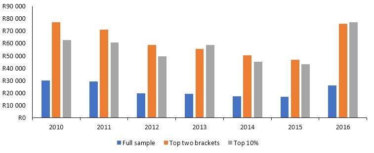
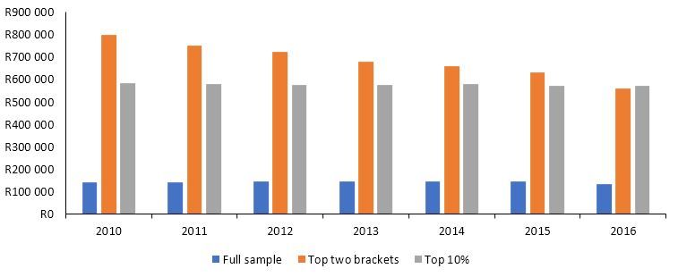
Figure 1 shows the absolute level of taxable (or reported) income over the sample for different income
groupings (expressed in constant 2010 prices). For the full universe of taxpayers, real taxable income
declined by 1 per cent per annum, on average, between 2010 and 2016. For the top two tax brackets, real
reported income declined by 5.8 per cent per annum, while for the top 10 per cent of income earners,
reported income declined by 0.5 per cent on average. While some of the decline in reported income
can be ascribed to the economic malaise experienced in South Africa over this period and its impact on
labour income, indications are that changing behaviour in the face of rising tax rates/burdens also played
an important role.
Figure 1: Taxable income (constant 2010 prices)
Source: author’s compilation, based on data from the National Treasury.
11Figure 2 shows the average tax bracket adjustments together with nominal (broad) income growth for
the top two income tax brackets across the sample period. Nominal income growth was larger than the
legislated adjustment in nominal tax brackets in four out of the six years under investigation, with the
largest divergence falling in 2016. This suggests that individuals in the second-highest tax bracket likely
migrated to a higher tax bracket, facing an increase in their marginal rate, while all taxpayers in the top
two income tax brackets faced significantly higher tax burdens. Additionally, the legislated marginal
tax rates for the top two income tax brackets were increased from 38 and 40 per cent to 39 and 41 per
cent, respectively, in the 2015/16 fiscal year. This likely prompted a behavioural response on the part of
taxpayers.
Figure 2: Bracket adjustment versus nominal income growth
Source: author’s compilation, based on data from the National Treasury and the South African Revenue Service.
This behavioural response is clearly visible when looking at the average level of deductions across the
sample. As mentioned above, the size of behavioural response to changing tax rates depends in large part
on the availability and use of deductions and exemptions. Figure 3 shows the average level of deductions
(expressed in constant 2010 prices) across the sample period.
Figure 3: Average level of deductions (constant 2010 prices)
Source: author’s compilation, based on data from the National Treasury.
The average level of deductions declined for most of the sample. However, there was a sharp increase
in 2016 for both the full sample and, in particular, at the top of the taxable income distribution. This
12corresponds to the smallest adjustment in nominal tax brackets over the sample period—average bracket
adjustments amounted to 2 per cent in the 2016/17 fiscal year, while the top two tax brackets saw no
adjustment. This, combined with a meaningful increase in nominal income, saw a significant increase
in the tax burden across the income distribution. This prompted a strong behavioural response in the
form of the increased use of deductions, reducing the level of reported income and the associated tax
liability.
To further enhance the intuition, it serves to split the sample into two. Table 5 gives elasticity estimates
for the top two income tax brackets and the top 10 per cent of income earners for the full sample, as well
as two sub-samples. The first sub-sample stacks the three-year differences for base year 2010 and 2011,
while the second stacks the three-year differences for base year 2012 and 2013.
Table 5: Elasticity estimates for various sub-samples
Full sample 2010/11 2012/13
Top two tax brackets (using taxable income cuts) 0.937 0.238 1.379
Standard deviation [0.009] [0.204] [0.260]
Top 10 per cent of income earners 0.497 0.126 0.868
Standard deviation [0.009] [0.077] [0.157]
Notes: estimates of 2SLS regressions. Regressions weighted by income. All income ranges based on base year income. All
regressions include log income, polynomials in base year income, and dummy variables for each base year.
Source: author’s compilation, based on data from the National Treasury.
As is clear from Table 5, the estimated elasticities for both the top two tax brackets and the top 10
per cent of income earners are much larger in the latter half of the sample and are also more precisely
estimated. This confirms the fact that changes in the tax structure over this period (including insufficient
bracket adjustment and changes in top marginal tax rates) induced significant behavioural responses on
the part of high-income earners.
The higher elasticity estimates in the latter half of the sample could also be a function of an increase in the
prevalence of tax avoidance and/or evasion. Over this period, the full extent of so-called ‘state capture’
and the deterioration in the efficiency of and trust in SARS had only just begun to make headlines. This
could have prompted an increase in both legal and illegal income shifting and/or avoidance measures.
Additionally, by 2016 the domestic economic situation had deteriorated dramatically, which might have
prompted high-income individuals to shift income offshore.
3.3 Optimal taxation
This section uses the framework described in Saez (2001, 2004) and Saez et al. (2012), summarized in
Giertz (2009) and Diamond and Saez (2011), and applied to South Africa in Kemp (2019) to calculate
the optimal marginal tax rates for high-income earners. The expression for the optimal rate τ ∗ is given
by:13
1−g
τ∗ = (5)
1−g+a·e
m
where a is the so-called Pareto parameter, denoted by zmz−z̄ with z̄ the reported income threshold (used
to split the sample according to income grouping), zm is the average income reported for individuals
earning above z̄, and g is the average marginal value of consumption for those earning more than z̄.
The latter is a complex function of society’s preferences. The parameter e is the estimated elasticity of
taxable or reported income.
13 See Kemp (2019) for details on the derivation.
13Using an ETI estimate of 0.37, and setting g = 0.28 and a = 2.13, Kemp (2019) calculates an optimal
marginal tax rate for the top 10 per cent of income earners in the relevant sample at 48 per cent. This
compares to legislated marginal tax rates of 38 and 40 per cent for the top two tax brackets. However,
as mentioned in Kemp (2019), the actual tax rate that should be compared to the theoretical benchmark
is not simply the legislated personal income tax rate. At a minimum, consumption taxes should also be
taken into consideration. Taking into account average consumption taxes over the sample period, the
corresponding actual effective marginal rates for the top two income tax brackets were 46.8 and 48.5 per
cent, respectively. This is largely in line with the calculated optimal rate.
Turning to the current sample, the Pareto parameter a for the top 10 per cent of income earners for the full
m
sample is calculated as a = zmz−z̄ = 2.09. This estimate compares favourably to others in the literature.14
Following Kiss (2013), g is set equal to the inverse of the ratio of the average income of the respective
income group to overall average income. For the top 10 per cent of income earners in the sample this
implies that g = 0.25. Substituting the values for a and g, as well as the elasticity estimate for the top
10 per cent of income earners, into Equation (5), the optimal marginal tax rate for the top 10 per cent of
income earners is estimated at 42 per cent. This is somewhat lower than the estimate in Kemp (2019),
reflecting the higher elasticity estimate. For the top two income tax brackets, the optimal marginal tax
rate (using the full sample) is estimated at 32 per cent (setting g = 0.21, a = 1.78, and e = 0.94). Again,
the lower estimate reflects the significantly higher ETI estimate for this group of taxpayers.
The marginal rate that should be compared to these theoretical benchmarks is then given by:15
τ = 1 − (1 − τcons ) · (1 − τ pit ) (6)
where τcons is the effective consumption tax rate and τ pit is the applicable marginal tax rate.
For the period 2010–14, consumption taxes averaged 14.7 per cent.16 Setting τcons = 14.7 per cent and
τ pit equal to 38 and 40 per cent produces actual effective marginal rates for the top two income tax
brackets of 47.3 and 49.0 per cent over this period. For the period 2015–16, consumption taxes averaged
15.6 per cent, while the top marginal tax rates were increased to 39 and 41 per cent, respectively. This
produces actual effective marginal rates for the top two income tax brackets of 48.2 and 49.9 per cent,
respectively. These marginal rates are much higher than the optimal rates estimated above, suggesting
that legislated marginal tax rates are significantly higher than the optimal revenue-maximizing level
(given the estimates for e, g, and a). This suggests that any expected revenue response from an increase
in legislated rates would be more than offset by the revenue impact of the behavioural response of
individual taxpayers. This is borne out by the persistent under-performance of total tax revenue relative
to expectations over recent years.
Turning to the different sub-samples, the divergence is even more stark. For the latter half of the sample,
the estimated optimal tax rate for the top 10 per cent of income earners is 29 per cent (with g = 0.25,
a = 2.10, and e = 0.87). For the top two income tax brackets, the optimal marginal tax rate is estimated
at 23 per cent (g = 0.23, a = 1.88, and e = 1.38). This reflects the significant increase in the behavioural
response of high-income earners to changing tax rates over this sub-sample.
14 Steenekamp (2012) estimates a value for a of 2.11 for the top 1 per cent of South African taxpayers, while Kemp (2019)
estimates a value of 2.13 for the top 10 per cent of income earners. This compares with estimates for the top 1 per cent of
income earners of 2.5 for Hungary (Kiss 2013), 1.8 for the United Kingdom (Brewer and Browne 2009), 1.6 for New Zealand
(New Zealand Treasury 2009), and 1.5 for the United States (Saez et al. 2012).
15 See Kemp (2019) for details.
16 See the Appendix for further information on the calculation of the effective consumption tax rates.
144 Conclusion
The paper used an updated dataset and a new sample to calculate updated estimates for the ETI for South
Africa
As in Kemp (2019), in the absence of any large tax reforms over the sample period, the phenomenon of
‘bracket creep’ was used to estimate the ETI. The elasticity for taxable income is estimated at around 0.4,
somewhat higher than the estimate presented in Kemp (2019). The elasticity for broad income is esti-
mated at around 0.2, similar in size to the earlier study. As in Kemp (2019), it was found that behavioural
responses are concentrated in higher-income groups as suggested by the higher elasticity estimates for
individuals in the top two income tax brackets and the top 10 per cent of income earners.
Using these elasticity estimates as an input in an optimal taxation framework, it is shown that current
legislated marginal tax rates for high-income earners are significantly higher than the optimal rate im-
plied by the ETI estimates, particularly with reference to the latter half of the sample. This reflects the
significant increase in the estimated elasticity over this period, precipitated by both insufficient adjust-
ments to the relevant tax brackets (i.e. adjustments did not compensate for nominal income growth) and
increases in legislated marginal tax rates.
The use of ‘bracket creep’ to identify the ETI is useful in the case in which large tax reforms are un-
available. However, the same caveats as discussed in Kemp (2019) apply. First, because ‘bracket creep’
is not a well-publicized legislated tax change, taxpayers may not be fully aware of the marginal tax
increases and thus might not respond to the change. Second, the identification technique does not allow
for the investigation of the anatomy of the behavioural response—that is, how different income sources
respond to tax rates. The current dataset would allow for the study of the possibly different responses of
different income sources (e.g. wage versus business versus interest income). This could provide insight
into which sources are responsible for the behavioural response at the level of taxable income.
In terms of future research, recent reforms to the tax structure, including the increase in the marginal
rates for the top two tax brackets in 2015/16 and the creation of a new top tax bracket with marginal rate
equal to 45 per cent, could conceivably be used to identify and estimate the ETI for high-income earners.
These reforms, in combination with the construction of a detailed microsimulation model, could also be
used to identify and estimate income effects.
References
Atkinson, A.B., and A. Leigh (2008). ‘Top Incomes In New Zealand 1921–2005: Understanding the
Effects of Marginal Tax Rates, Migration Threat, and the Macroeconomy’. Review of Income and
Wealth, 54(2): 149–65.
Auten, G., and R. Carroll (1999). The Effect of Income Taxes on Household Income. Review of Eco-
nomics and Statistics, 81(4): 681–93.
Auten, G., R. Carroll, and G. Gee (2008). ‘The 2001 and 2003 Tax Rate Reductions: An Overview and
Estimate of the Taxable Income Response’. National Tax Journal, 61(3): 345–64.
Brewer, M., and J. Browne (2009). ‘Can More Revenue be Raised by Increasing Income Tax Rates for
the Very Rich?’ IFS Briefing Note BN84. London: Institute for Fiscal Studies.
Brewer, M., E. Saez, and A. Shephard (2010). ‘Means-Testing and Tax Rates on Earnings’. In S. Adam,
T. Besley, R. Blundell, S. Bond, R. Chote, M. Gammie, P. Johnson, G. Myles, and J. Poterba (eds),
Dimensions of Tax Design: The Mirrlees Review, vol. 1. Oxford: Oxford University Press.
15Chetty, R., J.N. Friedman, T. Olsen, and L. Pistaferri (2011). ‘Adjustment Costs, Firm Responses, and
Micro vs. Macro Labor Supply Elasticities: Evidence from Danish Tax Records’. Quarterly Journal
of Economics, 126(2): 749–804.
Creedy, J. (2009). ‘The Elasticity of Taxable Income: An Introduction’. Department of Economics
Working Paper 1085. Melbourne: University of Melbourne.
Diamond, P.A., and E. Saez (2011). ‘The Case for a Progressive Tax: From Basic Research to Policy
Recommendations’. CESifo Working Paper 3548. Munich: CESifo Group.
Ebrahim, A., and C. Axelson (2019). ‘The Creation of an Individual Panel Using Administrative Tax
Microdata in South Africa’. UNU-WIDER Working Paper 2019/27. Helsinki: UNU-WIDER.
Ebrahim, A., R. Gcabo, L. Khumalo, and J. Pirttilä (2019). ‘Tax Research in South Africa’. UNU-
WIDER Working Paper 2019/9. Helsinki: UNU-WIDER.
Feldstein, M. (1995). ‘The Effect of Marginal Tax Rates on Taxable Income: A Panel Study of the 1986
Tax Reform Act’. Journal of Political Economy, 103(3): 551–72.
Giertz, S.H. (2007). ‘The Elasticity of Taxable Income over the 1980s and 1990s’. National Tax Journal,
60(4): 743–68.
Giertz, S.H. (2009). ‘The Elasticity of Taxable Income: Influences on Economic Efficiency and Tax
Revenues, and Implications for Tax Policy’. In A.D. Viard (ed.), Tax Policy Lessons from the 2000s.
Washington, DC: AEI Press.
Gorodnichenko, Y., J. Martinez-Vazquez, and K.S. Peter (2009). ‘Myth and Reality of Flat Tax Re-
form: Micro Estimates of Tax Evasion Response and Welfare Effects in Russia’. Journal of Political
Economy, 117(3): 504–54.
Gottfried, P., and H. Schellhorn (2004). ‘Empirical Evidence on the Effects of Marginal Tax Rates on In-
come: The German Case’. IAW Discussion Paper 15. Tübingen: Institut für Angewandte Wirtschafts-
forschung (IAW).
Gruber, J., and E. Saez (2002). ‘The Elasticity of Taxable Income: Evidence and Implications’. Journal
of Public Economics, 84(1): 1–32.
Hansson, A.A. (2007). ‘Taxpayers’ Responsiveness to Tax Rate Changes and Implications for the Cost
of Taxation in Sweden’. International Tax and Public Finance, 14(5): 563–82.
Kemp, J.H. (2019). ‘The Elasticity of Taxable Income: The Case of South Africa’. South African Journal
of Economics, 87(4): 417–49.
Kiss, A. (2013). ‘The Optimal Top Marginal Tax Rate: Application to Hungary’. European Journal of
Government and Economics, 2(2): 100–18.
Kleven, H.J., and E.A. Schultz (2014). ‘Estimating Taxable Income Responses Using Danish Tax Re-
forms’. American Economic Journal: Economic Policy, 6(4): 271–301.
Kopczuk, W. (2005). ‘Tax Bases, Tax Rates and the Elasticity of Reported Income’. Journal of Public
Economics, 89(11–12): 2093–2119.
Kopczuk, W., J. Friedman, H. Galper, M. Manacorda, E. Saez, D. Silverman, and J. Slemrod (2012).
‘The Polish Business “Flat” Tax and Its Effect on Reported Incomes: A Pareto Improving Tax Re-
form?’ Columbia University Working Paper. New York: Columbia University.
Moffitt, R.A., and M. Wilhelm (2000). ‘Taxation and the Labor Supply: Decisions of the Affluent’.
Working Paper 6621. Cambridge, MA: NBER.
16New Zealand Treasury (2009). ‘Estimating the Distortionary Costs of Income Taxation in
New Zealand.’ Background Paper for Session 5 of the Victoria University of Welling-
ton Tax Working Group. Wellington: Victoria University of Wellington. Available at:
www.victoria.ac.nz/sacl/centres-and-institutes/cagtr/twg/publications/
5-estimating-the-distortionary-costs-of-income-taxation-in-newzealand-treasury.
pdf.
Pieterse, D., E. Gavin, and C.F. Kreuser (2018). ‘Introduction to the South African Revenue Service and
National Treasury Firm-Level Panel’. South African Journal of Economics, 86(S1): 6–39.
Piketty, T. (1999). ‘Les hauts revenus face aux modifications des taux marginaux supérieurs de l’impôt
sur le revenu en France, 1970–1996’. Économie et Prévision, 138(2): 25–60.
Pirttilä, J., and H. Selin (2006). ‘How Successful is the Dual Income Tax? Evidence from the Finnish
Tax Reform of 1993’. CESifo Working Paper 1875. Munich: CESifo Group.
Saez, E. (2001). ‘Using Elasticities to Derive Optimal Income Tax Rates’. Review of Economic Studies,
68(1): 205–29.
Saez, E. (2003). ‘The Effect of Marginal Tax Rates on Income: A Panel Study of “Bracket Creep”’.
Journal of Public Economics, 87(5–6): 1231–58.
Saez, E. (2004). ‘Reported Incomes and Marginal Tax Rates, 1960–2000: Evidence and Policy Implica-
tions’. Working Paper 10273. Cambridge, MA: NBER.
Saez, E. (2010). ‘Do Taxpayers Bunch at Kink Points?’. American Economic Journal: Economic Policy,
2(3): 180–212.
Saez, E., and M.R. Veall (2005). ‘The Evolution of High Incomes in Northern America: Lessons from
Canadian Evidence’. American Economic Review, 95(3): 831–49.
Saez, E., J. Slemrod, and S.H. Giertz (2012). ‘The Elasticity of Taxable Income with Respect to Marginal
Tax Rates: A Critical Review’. Journal of Economic Literature, 50(1): 3–50.
Saez, E., J.B. Slemrod, and S.H. Giertz (2009). ‘The Elasticity of Taxable Income with Respect to
Marginal Tax Rates: A Critical Review’. Working Paper 15012. Cambridge, MA: NBER.
Selén, J. (2002). ‘Taxable Income Responses to Tax Changes: A Panel Analysis of the 1990/91 Swedish
Reform’. Working Paper 177. Stockholm: Trade Union Institute for Economic Research.
Sillamaa, M.-A., and M.R. Veall (2001). ‘The Effect of Marginal Tax Rates on Taxable Income: A Panel
Study of the 1988 Tax Flattening in Canada’. Journal of Public Economics, 80(3): 341–56.
Singleton, P. (2011). ‘The Effect of Taxes on Taxable Earnings: Evidence from the 2001 and Related
U.S. Federal Tax Acts’. National Tax Journal, 64(2): 323–51.
Steenekamp, T. (2012). ‘Taxing the Rich at Higher Rates in South Africa?’. Southern African Business
Review, 16(3): 1–29.
Thoresen, T.O., and Vattø, T.E. (2013). ‘Validation of Structural Labor Supply Model by the Elasticity
of Taxable Income’. Discussion Paper 738. Oslo: Statistics Norway, Research Department.
Van Heerden, Y. (2013). ‘Personal Income Tax Reform to Secure the South African Revenue Base
Using a Micro-simulation Tax Model’. PhD thesis. Pretoria: Faculty of Economic and Management
Sciences, University of Pretoria.
Weber, C.E. (2014). ‘Toward Obtaining a Consistent Estimate of the Elasticity of Taxable Income Using
Difference-in-Differences’. Journal of Public Economics, 117(C): 90–103.
17You can also read