Traffic Flow Prediction with Vehicle Trajectories - wands @ ntu
←
→
Page content transcription
If your browser does not render page correctly, please read the page content below
Traffic Flow Prediction with Vehicle Trajectories
 Mingqian Li,13 * Panrong Tong,12 Mo Li,12 Zhongming Jin,3 Jianqiang Huang,13 Xian-Sheng Hua3
               1
              Alibaba-NTU Singapore Joint Research Institute, Nanyang Technological University, Singapore
                   2
                School of Computer Science and Engineering, Nanyang Technological University, Singapore
                                                  3
                                                    Alibaba Group
      {mingqian001, tong0091, limo}@ntu.edu.sg, {zhongming.jinzm, jianqiang.hjq, xiansheng.hxs}@alibaba-inc.com

                            Abstract
  This paper proposes a spatiotemporal deep learning frame-
  work, Trajectory-based Graph Neural Network (TrGNN), that
                                                                                                                       ?
  mines the underlying causality of flows from historical vehi-
  cle trajectories and incorporates that into road traffic predic-
                                                                                                                     ? ?
  tion. The vehicle trajectory transition patterns are studied to            Regular pattern           Non-recurrent pattern
  explicitly model the spatial traffic demand via graph propa-
  gation along the road network; an attention mechanism is de-                (a) When only flow observations are available
  signed to learn the temporal dependencies based on neighbor-
  hood traffic status; and finally, a fusion of multi-step predic-
  tion is integrated into the graph neural network design. The
  proposed approach is evaluated with a real-world trajectory
  dataset. Experiment results show that the proposed TrGNN
  model achieves over 5% error reduction when compared with
  the state-of-the-art approaches across all metrics for normal             Regular pattern             Non-recurrent pattern
  traffic, and up to 14% for atypical traffic during peak hours or             (b) When vehicle trajectories are available
  abnormal events. The advantage of trajectory transitions es-
  pecially manifest itself in inferring high fluctuation of flows    Figure 1: The challenge in predicting non-recurrent traffic
  as well as non-recurrent flow patterns.                            flows and how vehicle trajectory information may help.

                       1   Introduction
Robust and accurate predictions of future vehicular traf-               According to studies in transportation domain (Skabardo-
fic conditions (e.g., flow, speed, density), either short-term       nis, Varaiya, and Petty 2003), the road traffic contains two
or long-term, is necessary for many transportation services          parts: recurrent traffic, which often arises from periodic traf-
such as traffic control and route planning. The challenge of         fic demand such as daily commuters during morning and
traffic prediction primarily stems from the complex nature           evening rush hours, and non-recurrent traffic, which is trig-
of spatiotemporal interactions among vehicles and the road           gered by unexpected causes such as public transit disrup-
network.                                                             tions or accidents. Existing approaches learn spatiotemporal
   Data driven approaches have been extensively exploited            traffic correlations from patterns that were seen in training
in predicting vehicular traffic on the road network. Early           data from history, and thus are favourable in predicting re-
attempts leverage time series analysis (Williams and Hoel            current traffic. In predicting non-recurrent traffic, however,
2003), which primarily models the temporal correlations of           existing approaches may fail to achieve the same level of
traffic. Conventional machine learning models (Sun, Zhang,           accuracy, mainly due to insufficient observations of similar
and Yu 2006) are applied to learn the spatiotemporal correla-        flow patterns in history. Figure 1(a) illustrates such an is-
tions of traffic from historical data. Latest works apply deep       sue with an example - when only flow observations (i.e., the
learning to traffic prediction, and they typically follow a spa-     number of vehicles passing each road segment) are avail-
tiotemporal framework, e.g., Graph Neural Network (GNN)              able, existing approaches may learn spatiotemporal correla-
(Li et al. 2018), which demonstrates superior capability in          tions of recurrent flow patterns among different road seg-
learning complicated spatiotemporal correlations.                    ments across different time, which cannot effectively reason
    * Mingqian Li is under the joint PhD Program with Al-
                                                                     how a previously unseen part of the traffic is credited to fu-
ibaba Group and Alibaba-NTU Singapore Joint Research Institute,
                                                                     ture road traffic.
Nanyang Technological University, Singapore.                            This paper targets at addressing the current challenge
Copyright © 2021, Association for the Advancement of Artificial      with non-recurrent traffic flow prediction - the challenge that
Intelligence (www.aaai.org). All rights reserved.                    historical flow data cannot provide insights on how non-
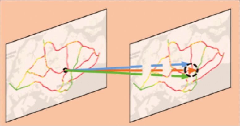
recurrent traffic flows correlate in time and space. Thus,         speed (Li et al. 2018), density (Raj, Bahuleyan, and Vana-
complementary to conventional spatiotemporal modeling              jakshi 2016), accident rate (Sun and Sun 2015), and arrival
using aggregated traffic flow observations, we also exploit        time (Zhou, Zheng, and Li 2012).
intact vehicle trajectories to infer short-term traffic depen-        Early attempts with time series analysis model the tempo-
dency. As suggested in Figure 1(b), trajectory data provide        ral correlations of traffic, such as SARIMA (Williams and
information of how each portion of a traffic flow transits         Hoel 2003) and VAR (Chandra and Al-Deek 2009). Those
from one road segment to another, and thus implies the de-         approaches rely on strong assumptions of linearity and sta-
pendency of upstream and downstream flows. The depen-              tionarity and often ignore the spatial impact from neighbor-
dency embeds knowledge of how downstream traffic are               ing traffic. Another line of research focuses on studies of
caused by upstream traffic and thus may help infer traffic         conventional machine learning models, such as k-NN (Davis
flow patterns that have not been seen before.                      and Nihan 1991), Bayesian network (Sun, Zhang, and Yu
   Incorporating trajectories to traffic flow prediction entails   2006), and SVR (Vanajakshi and Rilett 2004). In those mod-
the following challenges: 1) trajectories are only observed        els, spatiotemporal features are manually designed and ex-
from historical data; 2) traffic patterns at trajectory level      tracted, and the models are often shallow in structure with
need be aggregated properly to reflect the traffic patterns        limited learning capability.
at flow level; and 3) future flows may deviate from ob-               Recent advances in deep learning have motivated its ap-
served patterns due to influence from the environment. To          plication in traffic prediction (Liu et al. 2018). Earlier neu-
address those challenges, this paper proposes a novel model,       ral network architectures include SAEs (Lv et al. 2014) and
Trajectory-based Graph Neural Network (TrGNN), which               DBN (Jia, Wu, and Du 2016). State-of-the-art approaches
learns trajectory transition patterns from historical trajecto-    typically follow a spatiotemporal framework: it models the
ries and incorporates that into a spatiotemporal graph-based       spatial correlations by CNNs (Yu, Yin, and Zhu 2018) view-
deep learning framework. The main contributions of this pa-        ing the map as an image, or by GCNs (Li et al. 2018) view-
per are summarized as follows:                                     ing the road network as a graph; and it models the tem-
                                                                   poral evolution of traffic as a sequence of signals (Zhao
• We identify the challenge of predicting non-recurrent traf-      et al. 2019a). The spatiotemporal framework makes it flex-
  fic flows, and we propose to incorporate vehicle trajectory      ible to embed auxiliary information such as weather con-
  data in traffic flow prediction. To the best of our knowl-       ditions (Yao et al. 2018), accident data (Yu et al. 2017),
  edge, this is the first study that attempts to leverage ve-      map query records (Liao et al. 2018), and POIs (Geng et al.
  hicle trajectory data to mine the underlying causality of        2019). Similar to these works, our model follows a graph-
  flows among roads.                                               based spatiotemporal deep learning framework; in addition,
• We design an end-to-end spatiotemporal graph-based               we incorporate vehicle trajectory data into the design to ad-
  deep learning model to predict traffic flows of the entire       dress the challenge of predicting non-recurrent flows.
  road network. Our model embeds trajectory transition into           Among deep learning approaches, Graph Wavenet (Wu
  graph propagation along the road network to model the            et al. 2019) and SLC (Zhang et al. 2020) mine latent graph
  spatial traffic demand; it learns the temporal dependen-         structures to capture long-range dependencies, and MRes-
  cies with an attention mechanism based on neighborhood           RGNN (Chen et al. 2019) designs a multiple hop scheme
  traffic status; and finally it fuses multi-step predictions.     to capture long-term periodic patterns; the design goals of
                                                                   those methods deviate from our key objective of predicting
• We conduct extensive experiments 1 with real-world vehi-         non-recurrent traffic which is often caused by sudden dis-
  cle trajectory data and the results suggest that our model       ruptions locally. Other methods explore temporal building
  outperforms state-of-the-art approaches in terms of pre-         blocks and combine them with graph convolution, e.g., at-
  diction errors across various scenarios (over 5% error           tention in ASTGCN (Guo et al. 2019) and GMAN (Zheng
  reduction), and is especially superior in predicting non-        et al. 2020), gated recurrent unit in T-GCN (Zhao et al.
  recurrent flow patterns, e.g., during abnormal events (up        2019a), temporal convolution in STGCN (Yu, Yin, and Zhu
  to 14% error reduction).                                         2018). Most of these methods aim at reducing overall predic-
   The rest of the paper is organized as follows. Section 2        tion errors without specific focus on non-recurrent traffic.
discusses related work on vehicular traffic prediction. Sec-          Few existing works leverage trajectory data in traffic flow
tion 3 defines the problem and introduces some preliminary         prediction. Zhang et al. leverages trajectories in traffic state
knowledge. The proposed model TrGNN is introduced in               estimation, only to calibrate the embedding of road intersec-
Section 4, and experimentally evaluated in Section 5. Sec-         tions (2019). In comparison, our work utilizes trajectories to
tion 6 concludes the paper.                                        mine the traffic flow transitions among road segments. Some
                                                                   work leverages trajectories for other purposes such as map
                                                                   generation (Ruan et al. 2020) which is less relevant to the
                    2   Related Work                               topic of our study.
For decades, data driven approaches have been exploited to
predict road traffic conditions, such as flow (Lv et al. 2014),                        3    Preliminaries
                                                                   We first define the problem of traffic flow prediction, and
   1                                                               then introduce some preliminary knowledge of Graph Con-
     Code      and    dummy      data are        available    at
https://github.com/mingqian000/TrGNN.                              volutional Networks (GCNs) and attention mechanism.
3.1   Problem Definition                                              Instead of directly learning θ to fuse different hops of traf-
In traffic flow prediction, the target is to predict future traffic   fic demand, we define an attention mechanism to learn the
flows given historical traffic flows on a static road network.        temporal weights, as illustrated in Section 3.3.
Definition 1 (Road Graph). The road network can be for-
mulated into a directed road graph G = (V, E, A). V =                 3.3   Attention Mechanism
{vi }i=1,2,...,M is a finite set of nodes where each node vi          In learning a weighted sum of values, an attention mecha-
represents a road segment i, and E = {eij } is a set of di-           nism (Vaswani et al. 2017; Veličković et al. 2018) replaces
rected edges where each edge eij = (vi , vj ) indicates that          the weight parameters with a learning module in which the
road segment i is an immediate upstream of road segment j,            same set of parameters (called keys) are shared across all
                M ×M
and A ∈ [0, 1]          represents the weighted road adjacency        values in calculating the weights. A typical formulation of
matrix. Each node vi has a self-loop, i.e., eii ∈ E.                  an attention mechanism given queries Q ∈ RN ×dk , keys
Definition 2 (Traffic Flows). Traffic flow is defined as the          K ∈ RM ×dk and values V ∈ RM ×dv is
number of vehicles passing by a road segment during a spe-
cific time interval. Given a road graph G = (V, E, A), we                     Attention(Q, K, V ) := sof tmax(QK | )V.            (4)
use X ∈ RT ×|V| to represent the time series of traffic flows,        In this paper, we apply the attention mechanism for a more
where for each interval t = 1, 2, ..., T , Xt ∈ R|V| represents       flexible fusion of traffic demand based on traffic status.
the traffic flows of all road segments in the road network dur-
ing time interval t.
                                                                                          4    Methodology
Definition 3 (Trajectory). Given a road graph G =
(V, E, A), we use T = (v1 , v2 , ..., vI ) to represent a tra-        In this section, we introduce our proposed model, TrGNN,
jectory of a vehicle, where each vi ∈ V represents a road             to address the problem of traffic flow prediction (Problem
segment in the trajectory, satisfying (vi , vi+1 ) ∈ E, vi 6=         1). The model follows a spatiotemporal framework, leverag-
vi+1 , ∀i = 1, 2, ..., I − 1.                                         ing trajectory transition patterns. The extraction of trajectory
Problem 1 (Traffic Flow Prediction). Given a road graph               transition is illustrated in Figure 2. An overview of the model
                                                                      architecture is illustrated in Figure 3. We elaborate each part
G = (V, E, A), find a prediction function fˆ with parameter
                                                                      of the architecture in the subsections below.
Θ such that given traffic flows X(t−Tin +1):t within a histor-
ical window period Tin up to time interval t, fˆ estimates the        4.1   Trajectory Transition
most likely traffic flows X̂t+1 for the next time interval t + 1,
i.e.,                                                                 Figure 1 illustrates the extra information gain from historical
                                                                      trajectory data when inferring non-recurrent traffic patterns.
         X̂t+1 := fˆΘ (Xt−Tin +1 , ..., Xt )                          Compared to flows, trajectories provide essential knowledge
                ≈ arg max log p(X |X                    ),     (1)    about drives’ origin and destination (O-D), and help infer
                                     t+1    (t−Tin +1):t
                    Xt+1                                              their choices of routes at road intersections. Figure 1(b)
                                                                      visualizes a contrast between green and dark red trajecto-
3.2   Graph Convolutional Networks (GCNs)                             ries, which indicates that vehicles coming from different up-
To model the spatial traffic demand, we leverage the idea of          stream road segments (or origins) may differ in their dis-
graph propagation from GCNs.                                          tributions of downstream road segments (or destinations).
   A GCN is defined over a graph G = (V, E, A). It ap-                Hence, for non-recurrent traffic patterns, we may infer flows
plies convolutional operations on graph signals in spectral           on a trajectory basis: first obtain the origins of the existing
domain (Kipf and Welling 2017; Defferrard, Bresson, and               vehicles, and then based on their origins, infer the distribu-
Vandergheynst 2016). Given a graph signal X ∈ R|V|×N                  tion of their destinations. In Figure 1(b), for example, we
where N is the number of features, a typical formulation of           may infer that the extra spike of flow is more likely caused
a K-hop graph convolutional layer is                                  by extra vehicle flow of dark red trajectories instead of green
                                     K
                                     X                                trajectories.
           GCNG (X; W, θ) = σ(             θk Lk X)W           (2)       We utilize historical trajectories to explicitly model the
                                     k=0                              transition of flows between upstream and downstream road
                  |V|×|V|                                             segments. Figure 2 illustrates the extraction of trajectory
where L ∈ [0, 1]          is the graph Laplacian, a variant of        transition. We view historical trajectories as Markov pro-
A, to control the graph propagation across nodes; θ ∈ RK              cesses, and by aggregating trajectories of all vehicles, we
controls the fusion of different hops; W ∈ RN ×M (M is                may infer the transition of flows from one road segment to
the output feature dimension) controls the fusion of different        others. The rest of this subsection elaborates the extraction
features; and σ is the activation function.                           of trajectory transition.
   In this paper, to model traffic demand and status, we                 The trajectory generation of a vehicle can be modeled as
adopt graph propagation (GraphProp), a simplified variant             a first-order Markov process, assuming that the transition
of GCN, with one single input feature (i.e., traffic flow) and        probability from each upstream road segment to each down-
thus ignoring the feature-wise parameters W :                         stream road segment is stationary across days. We define a
 GraphP rop(X, A; K) := [XkAXkA2 Xk...kAK X]. (3)                     trajectory transition tensor P ∈ RTd ×|V|×|V| , where each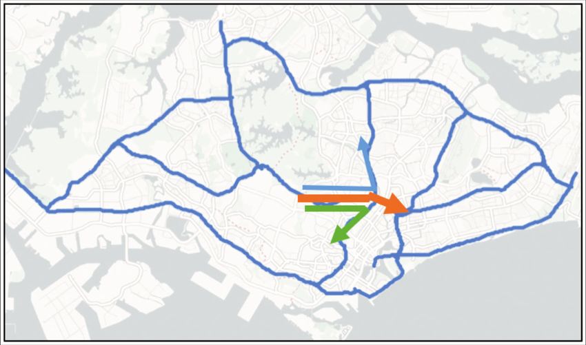
vehicles                 trajectories                                        time

                                                                                                                             !",$,%
                            …
                                                                                                                           !",$,'     !",$,&

           Historical trajectories                                   Trajectory inference                          Trajectory transition !

                                     Figure 2: Learning trajectory transition from historical trajectories.

Pt ∈ R|V|×|V| represents the trajectory transition probabili-                      demand Dt ∈ R|V|×(d+1) via graph propagation:
ties for the tth time interval of the day. The trajectory gener-
ation process can be represented as                                                         Dt = GraphP rop(Xt , Pt| ; d)
                                                                                                                                                   (7)
                                                                                               = [Xt k Pt| Xt k (Pt| )2 Xt k ... k (Pt| )d Xt ],
                 P (T |t) = P ((v1 , v2 , ..., vI )|t)
                                     I−1
                                     Y                                             where k denotes concatenation, ·| denotes matrix transpose,
                          = π(v1 )         P (vi+1 |vi ; t)                        and parameter d stands for demand hop, controlling the far-
                                     i=1                                 (5)       thest possible destination.
                                     I−1
                                     Y                                                The graph propagation simulates the propagation of flows
                          = π(v1 )         Pt,vi ,vi+1 .                           along the road network, and as a result, the traffic demand
                                     i=1                                           D is an aggregation of the short-range and long-range desti-
                                                                                   nations (in different hops) of all vehicles in existing flows.
Alternatively, P can be derived from a higher-order Markov
process, which would require larger sample size and higher
                                                                                   4.3      Temporal Modeling of Traffic Demand based
computational complexity.
   To estimate tensor P, we collect historical trajectories of
                                                                                            on Traffic Status
all vehicles from the training set, and aggregate the cumu-                        The modeling of traffic demand in Section 4.2, however,
lative transition probability with respect to time of day, up-                     does not consider the propagation speed of flows, which
stream road segment, and downstream road segment:                                  should depend on traffic status. Traffic status refers to the
                                                                                   overall traffic volume in the neighboring of each road seg-
                 #vehicles (vi → vj |t) + 1[vj ∈ N(vi )]                           ment. If the traffic status is congested around a road seg-
  P̂t,vi ,vj =                                           , (6)
                     #vehicles(vi |t) + kN(vi )k                                   ment (i.e., high volume of flows in the neighboring road
                                                                                   segments), the propagation of flows along that road segment
where t stands for the tth time interval of day, and N(vi )                        should be slow, and vice versa.
denotes the set of downstream neighbors of road segment                               A temporal module is thus designed to infer how each
vi . To mitigate data sparsity, P̂ is smoothed out by adding a                     hop of traffic demand, from short range to long range, corre-
constant 1 for any pair of consecutive road segments.                              sponds to the future traffic flow in the targeted time interval.
    The trajectory transition tensor P summarizes the proba-                       This is done by assigning a weight to each hop of traffic
bility distribution of drivers’ choices of routes. In a macro-                     demand via an attention mechanism (Section 3.3) based on
scopic view, it approximates the transition of flows from                          traffic status. Thus, we first obtain traffic status, and then
upstream to downstream road segments in near future, and                           build an attention mechanism based on traffic status.
serves as a lookup table in the proposed TrGNN model.                                 For each input time interval t, we obtain traffic status
                                                                                                   s+1
                                                                                   St ∈ R|V|×(2 −1) via graph propagation in s hops from
4.2   Spatial Modeling of Traffic Demand                                           neighboring road segments. The graph propagation is done
Based on trajectory transition, we design a graph propaga-                         via dual random walk to incorporate both upstream and
tion mechanism to infer the traffic demand in the spatial                          downstream traffic:
domain. Traffic demand refers to the short-range and long-
                                                                                      St = GraphP ropdual (Xt , Ã; s)
range destinations of existing vehicles on the road network.                                                                                       (8)
   We leverage graph propagation from Graph Convolu-                                        = [Xt k Ã| Xt k ÃXt k Ã| Ã| Xt k ... k Ãs Xt ],
tional Networks (Section 3.2) to simulate the transition of
vehicles along the road network. We perform graph propa-                           where à is a normalized variant of the weighted road adja-
gation in d hops, resulting in a graph of traffic demand for                       cency matrix A, and parameter s stands for status hop, con-
each hop. For each input time interval t, we can derive traffic                    trolling the radius of the neighborhood.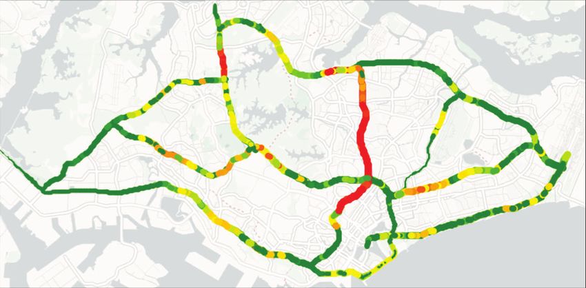
t                        t
                                                                                                           t
                                      Graph Propagation           Traffic demand "#
      Trajectory transition &
        t                                                                                                  Predicted flows !

                                                                                          Road-wise        Multi-step fusion
                                      Graph Propagation                                   Temporal
        Historical flows '                                        Traffic status %#
                                                                                          Attention
                                                                                                          t+1

                                                                                                          Predicted flows $
        Road adjacency (

Figure 3: Trajectory-based Graph Neural Networks (TrGNN). The framework models spatial traffic demand via graph propaga-
tion based on trajectory transition, and models temporal dependencies via attention mechanism based on neighborhood traffic
status. The final prediction is a fusion of multi-step prediction.

   We apply a road-wise attention mechanism (referring to              also depend on new vehicles entering the road network (e.g.,
the dot-product attention in (Vaswani et al. 2017)) param-             entering from the boundary of the region, or entering from
                                 s+1
eterized by keys K ∈ R|V|×(2 −1)×(d+1) , taking traffic                a local road to an arterial road) and existing vehicles leav-
status St as queries and traffic demand Dt as values, to as-           ing the road network, which we call boundary flows. Since
sign weights α ∈ [0, 1]
                        |V|×(d+1)
                                   to different hops in traffic        the boundary flows are strongly associated with drivers’ O-D
demand Dt and take the weighted sum as an initial predic-              demand which is periodic, we embed some periodic features
                                                                       (e.g., time of day, is working day) into the multi-step fusion
tion of flows Ht ∈ R|V| :
                                                                       module to model the boundary flows.
           Ht = Attention(St , Dt ; K)
                    d
                    X                                                                 5    Experimental Evaluation
                =         α:,i   Dt,:,i                                5.1    Dataset Description
                    i=0                                     (9)
                    d
                                                                       We evaluate our model with SG-TAXI, a real-world dataset
                    X                                                  comprising GPS mobility traces from over 20,000 taxis
                =     [sof tmax(St ◦ K)]:,i        Dt,:,i              in Singapore. The dataset is provided by Singapore Land
                    i=0
                                                                       Transport Authority. We collect the GPS readings of all ac-
where sof tmax(·) is applied over the dimension of demand              tive taxis for a period of 8 weeks (14th Mar-8th May 2016).
hop, ◦ denotes road-wise matrix product, and       denotes             Each GPS reading comprises vehicle id, longitude, latitude,
element-wise (or Hadamard) product.                                    and timestamp. The road network comprises 2,404 road seg-
                                                                       ments, covering all expressways in Singapore.
4.4     Multi-Step Fusion
From a sequence of input flows {Xi }i=t−Tin +1,...,t , we ob-          5.2    Data Preprocessing
tain a sequence of initial predictions H ∈ RTin ×|V| . The            We preprocess the SG-TAXI dataset in 4 steps:
final layer of the model is a temporal fusion of H. We adopt
                                                                      1. Road graph formulation. For the road graph G =
a road-wise fully connected layer. For each road segment v,
                                                                         (V, E, A), we calculate the weighted road adjacency ma-
               yv := Xt+1,v                                              trix A as the exponential decay of distance between roads.
                  = F ullyConnected(H:,v ; Θ)            (10)         2. Map matching. We apply the Hidden Markov map
                      |
                  = Θ H:,v .                                             matching algorithm (Newson and Krumm 2009) to cor-
Alternatively, this layer can be replaced by any RNN cell                rect GPS readings to their corresponding road segments.
such as LSTM (Hochreiter and Schmidhuber 1997) or GRU                 3. Trajectory cleansing. Given a sequence of mapped GPS
(Chung et al. 2014)), or sequence modeling (Sutskever,                   points, we cleanse the vehicle’s trajectory as follows: 1)
Vinyals, and Le 2014), for a longer-term prediction.                     eliminate duplicate records; 2) if GPS reading is off for
   As a side note, the conservation of vehicles on the road              over 10 minutes (e.g., the driver turns off the sensing de-
network does not hold in practice. Future flows not only de-             vice), split the trajectory; 3) if driver stays on the same
pend on trajectory transition within the road network, but               road segment for over 2 minutes, split the trajectory; 4) if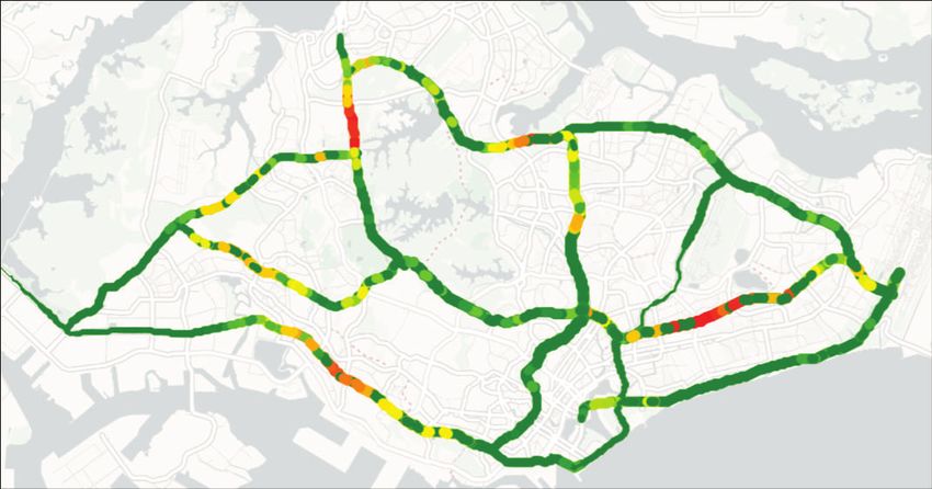
no path exists between two consecutive GPS points (e.g.,         5.5   Evaluation Metrics
   driver drives off the road network), split the trajectory;       We evaluate prediction results by three error metrics: MAE
   and 5) remove GPS points with extreme speed (i.e., speed         (Mean Absolute Error), MAPE (Mean Absolute Percentage
   derived from two consecutive GPS points exceeds 120              Error), and RMSE (Root Mean Squared Error), same as in
   km/hr). Finally, we recover the full trajectory via Dijk-        (Li et al. 2018). Lower errors indicate better performance.
   stra’s algorithm (Dijkstra et al. 1959).
                                                                    5.6   Results and Analysis
4. Flow aggregation. We aggregate trajectories into flows           Table 1 summarizes the evaluation of different approaches
   per road segment per 15-minute interval. We calibrate            for traffic flow prediction on SG-TAXI dataset. The com-
   flows to correct the daily fluctuation in taxi arrangement       parison covers overall testing as well as specific scenarios
   and better represent the overall traffic flows in Singapore.     including peak hours, non-peak hours and MRT breakdown.
                                                                       Overall Performance. According to Table 1, the overall
5.3    Experiment Settings                                          prediction errors of our model TrGNN are 26.43/0.30/38.65
                                                                    vph for MAE/MAPE/RMSE, and TrGNN achieves over 5%
The model is trained on the preprocessed SG-TAXI dataset.           error reduction from baselines across all metrics. The naive
The train-validate-test split is 5-1-2 week. Each data point        baselines generally give high errors, as they consider only
consists of input flows for 4 intervals (i.e., 1 hour) and output   temporal correlations of flows; MA is more accurate than
flows for 1 interval (i.e., 15 minute). Flows are normalized        HA, indicating that near-past flows play a stronger role than
before being input into the model. For hyperparameters, the         periodicity. VAR and RF perform better than the naive base-
demand hop d is set to 75, i.e., the maximum number of road         lines, as they incorporate neighborhood flows to model spa-
segments that a vehicle with a normal speed could traverse          tial correlations; in particular, RF performs better than VAR,
within a 15-minute interval, and the status hop s is set to 3.      implying that flows are not linearly correlated. For deep
   The model is implemented in PyTorch (Paszke et al. 2019)         learning, DCRNN achieves the best results out of all base-
on a single Tesla P100 GPU and is trained using Adam op-            lines, indicating the capability of graph-based deep learning
timizer (Kingma and Ba 2014) to minimize MSE loss. The              in capturing the spatiotemporal correlations. Finally, TrGNN
learning rate is initially set to 0.004 and is halved every 30      outperforms all existing baselines in all metrics, which veri-
epochs. The maximum epochs to train is set to 100. Early            fies the effectiveness of learning spatiotemporal transition of
stopping is applied on validation MAE. The training takes           flows from trajectories.
less than 4GB RAM and less than 1GB GPU memory.                        The line plot in Figure 4 visualizes predicted flows of
                                                                    TrGNN and a few representative baselines. HA fits the worst
                                                                    to the ground truths, implying high variation of flows from
5.4    Baseline Approaches                                          week to week; while TrGNN and DCRNN are more sensi-
                                                                    tive to the real-time fluctuations of flows. If we look further
Our model TrGNN is compared to representative baseline              into the peak hours indicated in the dashed box, TrGNN cap-
methods of each type, including naive methods (HA, MA),             tures the fluctuations of flows slightly earlier than DCRNN.
time series analysis (VAR), conventional machine learn-                Peak hours and non-peak hours. We select two typi-
ing (RF), and deep learning (T-GCN, STGCN, DCRNN).                  cal periods for experiments: peak hours (8-10pm on work-
Specifically, (i) HA (Historical Average) is the average flow       ing days, when public transport services become limited and
of the same time on the same day in the past four weeks;            the demand for taxis increases, thus with high fluctuation of
(ii) MA (Moving Average) is the average flow of the pre-            flows); and non-peak hours (2-4pm on working days when
vious 1 hour; (iii) VAR (Vector Auto-Regression) (Hamil-            people stay at offices and the demand for taxis stabilizes,
ton 1994) models the future flow as a linear combination            thus with low fluctuation of flows). Results are summarized
of historical flows in 5-hop neighborhood, implemented in           in Table 1 (under “Peak hours” and “Non-peak hours” col-
StatsModels (Seabold and Perktold 2010); (iv) RF (Random            umn). In peak hours, absolute errors (MAE/RMSE) are con-
Forest) is a decision-tree-based ensemble method that fits a        sistently higher than in overall testing; while in non-peak
piece-wise function on historical flows in 5-hop neighbor-          hours, the results are the opposite. This meets our expecta-
hood, implemented in Scikit-learn (Pedregosa et al. 2011)           tion, as predicting peak hour flows is more challenging due
with 100 trees; (vi) T-GCN (Temporal Graph Convolutional            to higher fluctuation in traffic demand. In both peak hours
Network) (Zhao et al. 2019a) is a graph-based neural net-           and non-peak hours, TrGNN outperforms all baselines, and
work that integrates GCN with GRU, implemented in Ten-              the error reduction of TrGNN is more significant during
sorflow (Zhao et al. 2019b); (vii) STGCN (Spatio-Temporal           peak hours (6-13% reductions on the performance metrics).
Graph Convolutional Networks) (Yu, Yin, and Zhu 2018) is               Figure 4 visualizes the heatmap snapshots of the predic-
a graph-based neural network that models both spatial and           tion errors of HA, DCRNN and TrGNN on the entire road
temporal dependencies via convolution, implemented in Py-           network during selected peak hours. The color indicates in-
torch (Opolka 2018); and (viii) DCRNN (Diffusion Con-               creasing prediction error from green to red. A comparison of
volutional Recurrent Neural Network) (Li et al. 2018) is a          the heatmap snapshots suggests the robustness of TrGNN in
graph-based neural network that integrates diffusion convo-         capturing the periodic fluctuation of flows in peak hours.
lution on graph with sequence learning, implemented in Py-             Abnormal event: MRT breakdown. We analyze an ab-
Torch (Shah 2019).                                                  normal event in Singapore, an MRT (Mass Rapid Transit)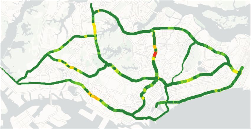
Overall                   Peak hours               Non-peak hours                    MRT breakdown
 Method MAE MAPE RMSE MAE MAPE RMSE MAE MAPE RMSE                                                      MAE MAPE RMSE
 HA         33.74       0.34     52.58 36.83      0.25     55.02 32.53        0.28   48.67             40.07   0.27   59.34
 MA         31.55       0.35     47.69 36.14      0.26     53.18 28.18        0.27   39.41             44.85   0.30   71.43
 VAR        29.27       0.33     43.22 34.23      0.24     49.71 28.10        0.26   39.28             40.68   0.27   64.41
 RF         29.26       0.33     43.38 34.13      0.24     49.75 27.53        0.26   38.53             42.28   0.28   66.53
 T-GCN      31.12       0.35     45.69 36.57      0.27     52.91 30.03        0.29   41.53             42.38   0.30   67.39
 STGCN 29.88            0.33     44.51 34.86      0.24     50.86 27.94        0.27   39.05             42.19   0.28   66.40
 DCRNN 29.01            0.31     43.12 33.74      0.25     48.88 27.75        0.27   38.74             40.39   0.28   64.28
 TrGNN- 27.34           0.31     40.05 31.35      0.23     45.11 26.61        0.26   37.20             38.57   0.27   59.53
 TrGNN 26.43            0.30     38.65 29.81      0.23     42.62 25.65        0.25   35.68             34.56   0.25   54.31
 %diff       -9%        -5%      -10% -12%         -6%     -13%      -7%      -4%     -7%              -14%    -8%     -8%
 Numbers in bold denote the best baseline performance and the best performance.
 %diff denotes the error reduction of TrGNN from the best baseline performance.

                  Table 1: Performance of different approaches for traffic flow prediction on SG-TAXI dataset.

       Non-peak hours Peak hours      Non-peak hours     Peak hours    Abnormal road segments
                                                                       at MRT breakdown

                                                                      Figure 5: Heatmap of abnormal flows in west Singapore due
                       DCRNN
                                                                      to MRT breakdown, and line plots of abnormal flows and
  HA                                             TrGNN
                                                                      predicted flows on a road segment. In heatmap, the color
                                                                      scale indicates the amount of extra flow compared to that of
                                                                      a normal day.
                        Prediction error (vph)

Figure 4: Line plot of predicted flows on the road network            instead of simply memorizing the historical flow patterns.
over a working day, and heatmap snapshots of prediction                  Component analysis: trajectory transition. To analyze
errors during peak hours.                                             the role of trajectory transition, we build a variant of TrGNN,
                                                                      TrGNN-, that replaces trajectory transition by the static road
                                                                      network. Results in Table 1 show that compared to TrGNN-
breakdown, when train services were disrupted due to power            , TrGNN reduces the prediction errors on all metrics in all
fault (Chew 2016). The disruption falls on a Monday night             scenarios, especially in MRT breakdown where MAE drops
lasting for more than one hour, and it affects 52 train stations      from 38.57 vph to 34.56 vph. This verifies the effectiveness
on 4 train lines, covering the whole area of west Singapore.          of trajectory transition in capturing flow dependency.
In Figure 5, the heatmap visualizes the abnormal spike of
flows of the affected region due to the increase in taxi de-                    6     Conclusion and Future Work
mand during the MRT breakdown period, and the line plot               This paper proposes a spatiotemporal deep learning model,
visualizes the predicted flows on a sample abnormal road              Trajectory-based Graph Neural Network (TrGNN), to solve
segment - TrGNN fits the best to the ground truths.                   the traffic flow prediction problem. The architecture lever-
   We select road segments within a 3km neighborhood of               ages historical trajectory transition as an input into the
any affected train station, and summarize their prediction re-        graph-based deep learning framework. TrGNN is evaluated
sults during the breakdown period in Table 1 (under “MRT              on SG-TAXI dataset. Results show that TrGNN outperforms
breakdown” column). Compared to “Overall”, we observe a               state-of-the-art approaches, especially being superior in pre-
significant increase in MAE for all baselines, ranging from           dicting non-recurrent traffic flows such as in MRT break-
19% to 44%, which demonstrates the performance drop in                down event. Potential future work includes expansion to a
predicting abnormal flows. Nevertheless, TrGNN outper-                higher-order Markov model, longer-term prediction, and op-
forms baselines by a significant error reduction of 14%. The          timization of computational complexity in extracting trajec-
result suggests the capability of TrGNN in capturing the spa-         tories. Moreover, our work points out a promising direction
tiotemporal causality even for non-recurrent flow patterns,           in incorporating trajectory data into traffic prediction.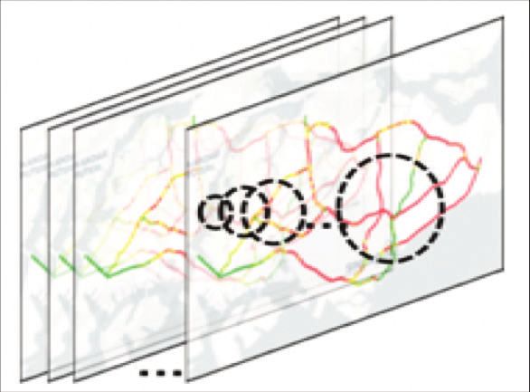
7    Acknowledgments                             Jia, Y.; Wu, J.; and Du, Y. 2016. Traffic Speed Prediction
This research is supported, in part, by NRF Singapore under      Using Deep Learning Method. In 2016 IEEE 19th Inter-
its grant SDSC-2019-001, Alibaba Group through Alibaba           national Conference on Intelligent Transportation Systems
Innovative Research (AIR) Program and Alibaba-NTU Sin-           (ITSC), 1217–1222. IEEE.
gapore Joint Research Institute (JRI), and Singapore MOE         Kingma, D. P.; and Ba, J. 2014. Adam: A Method for
Tier 1 grant RG18/20. Any opinions, findings and conclu-         Stochastic Optimization. arXiv preprint arXiv:1412.6980 .
sions or recommendations expressed in this material are          Kipf, T. N.; and Welling, M. 2017. Semi-Supervised Clas-
those of the author(s) and do not reflect the views of funding   sification with Graph Convolutional Networks. In Interna-
agencies.                                                        tional Conference on Learning Representations (ICLR).
                       References                                Li, Y.; Yu, R.; Shahabi, C.; and Liu, Y. 2018. Diffusion Con-
                                                                 volutional Recurrent Neural Network: Data-Driven Traffic
Chandra, S. R.; and Al-Deek, H. 2009. Predictions of Free-       Forecasting. In International Conference on Learning Rep-
way Traffic Speeds and Volumes Using Vector Autoregres-          resentations (ICLR).
sive Models. Journal of Intelligent Transportation Systems
13(2): 53–72.                                                    Liao, B.; Zhang, J.; Wu, C.; McIlwraith, D.; Chen, T.; Yang,
                                                                 S.; Guo, Y.; and Wu, F. 2018. Deep Sequence Learning with
Chen, C.; Li, K.; Teo, S. G.; Zou, X.; Wang, K.; Wang, J.;       Auxiliary Information for Traffic Prediction. In Proceed-
and Zeng, Z. 2019. Gated Residual Recurrent Graph Neural         ings of the 24th ACM SIGKDD International Conference on
Networks for Traffic Prediction. In Proceedings of the AAAI      Knowledge Discovery & Data Mining, 537–546.
Conference on Artificial Intelligence, volume 33, 485–492.
                                                                 Liu, Z.; Li, Z.; Wu, K.; and Li, M. 2018. Urban Traffic Pre-
Chew, H. M. 2016.          Train Service Disruptions on          diction from Mobility Data Using Deep Learning. IEEE Net-
Three MRT Lines and Bukit Panjang LRT Due                        work 32(4): 40–46.
to Power Fault: SMRT.           The Straits Times URL
https://www.straitstimes.com/singapore/transport/train-          Lv, Y.; Duan, Y.; Kang, W.; Li, Z.; and Wang, F.-Y. 2014.
disruption-on-east-west-line-and-north-south-line-due-to-        Traffic Flow Prediction With Big Data: A Deep Learning
traction-power.                                                  Approach. IEEE Transactions on Intelligent Transportation
                                                                 Systems 16(2): 865–873.
Chung, J.; Gulcehre, C.; Cho, K.; and Bengio, Y. 2014. Em-
pirical Evaluation of Gated Recurrent Neural Networks on         Newson, P.; and Krumm, J. 2009. Hidden Markov Map
Sequence Modeling. arXiv preprint arXiv:1412.3555 .              Matching Through Noise and Sparseness. In Proceedings
                                                                 of the 17th ACM SIGSPATIAL International Conference on
Davis, G. A.; and Nihan, N. L. 1991. Nonparametric Regres-       Advances in Geographic Information Systems, 336–343.
sion and Short-term Freeway Traffic Forecasting. Journal of
Transportation Engineering 117(2): 178–188.                      Opolka, F. 2018. Implementation of Spatio-Temporal Graph
                                                                 Convolutional Network with PyTorch. https://github.com/
Defferrard, M.; Bresson, X.; and Vandergheynst, P. 2016.         FelixOpolka/STGCN-PyTorch.
Convolutional Neural Networks on Graphs with Fast Local-
ized Spectral Filtering. In Lee, D.; Sugiyama, M.; Luxburg,      Paszke, A.; Gross, S.; Massa, F.; Lerer, A.; Bradbury, J.;
U.; Guyon, I.; and Garnett, R., eds., Advances in Neural In-     Chanan, G.; Killeen, T.; Lin, Z.; Gimelshein, N.; Antiga,
formation Processing Systems, volume 29, 3844–3852. Cur-         L.; et al. 2019. PyTorch: An Imperative Style, High-
ran Associates, Inc.                                             Performance Deep Learning Library. In Advances in Neural
                                                                 Information Processing Systems, 8026–8037.
Dijkstra, E. W.; et al. 1959. A Note on Two Problems
                                                                 Pedregosa, F.; Varoquaux, G.; Gramfort, A.; Michel, V.;
in Connexion with Graphs. Numerische Mathematik 1(1):
                                                                 Thirion, B.; Grisel, O.; Blondel, M.; Prettenhofer, P.; Weiss,
269–271.
                                                                 R.; Dubourg, V.; Vanderplas, J.; Passos, A.; Cournapeau, D.;
Geng, X.; Li, Y.; Wang, L.; Zhang, L.; Yang, Q.; Ye, J.; and     Brucher, M.; Perrot, M.; and Duchesnay, E. 2011. Scikit-
Liu, Y. 2019. Spatiotemporal Multi-Graph Convolution Net-        learn: Machine Learning in Python. Journal of Machine
work for Ride-Hailing Demand Forecasting. In Proceed-            Learning Research 12: 2825–2830.
ings of the AAAI Conference on Artificial Intelligence, vol-
                                                                 Raj, J.; Bahuleyan, H.; and Vanajakshi, L. D. 2016. Applica-
ume 33, 3656–3663.
                                                                 tion of Data Mining Techniques for Traffic Density Estima-
Guo, S.; Lin, Y.; Feng, N.; Song, C.; and Wan, H. 2019. At-      tion and Prediction. Transportation Research Procedia 17:
tention Based Spatial-Temporal Graph Convolutional Net-          321–330.
works for Traffic Flow Forecasting. In Proceedings of the
                                                                 Ruan, S.; Long, C.; Bao, J.; Li, C.; Yu, Z.; Li, R.; Liang,
AAAI Conference on Artificial Intelligence, volume 33, 922–
                                                                 Y.; He, T.; and Zheng, Y. 2020. Learning to Generate Maps
929.
                                                                 from Trajectories. Proceedings of the AAAI Conference on
Hamilton, J. D. 1994. Time Series Analysis, volume 2.            Artificial Intelligence 34(01): 890–897.
Princeton University Press Princeton, NJ.                        Seabold, S.; and Perktold, J. 2010. Statsmodels: Economet-
Hochreiter, S.; and Schmidhuber, J. 1997. Long Short-term        ric and Statistical Modeling with Python. In 9th Python in
Memory. Neural computation 9(8): 1735–1780.                      Science Conference.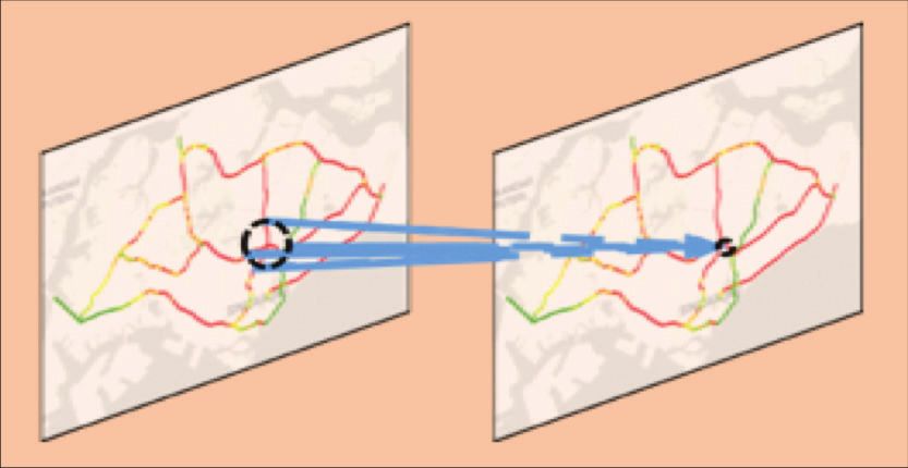
Shah, C. 2019. Diffusion Convolutional Recurrent Neural          Zhao, L.; Song, Y.; Zhang, C.; Liu, Y.; Wang, P.; Lin, T.;
Network Implementation in PyTorch. https://github.com/           Deng, M.; and Li, H. 2019a. T-GCN: A Temporal Graph
chnsh/DCRNN PyTorch.                                             Convolutional Network for Traffic Prediction. IEEE Trans-
Skabardonis, A.; Varaiya, P.; and Petty, K. F. 2003. Measur-     actions on Intelligent Transportation Systems .
ing Recurrent and Nonrecurrent Traffic Congestion. Trans-        Zhao, L.; Song, Y.; Zhang, C.; Liu, Y.; Wang, P.; Lin, T.;
portation Research Record 1856(1): 118–124.                      Deng, M.; and Li, H. 2019b. T-GCN: A Temporal Graph
Sun, J.; and Sun, J. 2015. A Dynamic Bayesian Network            Convolutional Network for Traffic Prediction. https://github.
Model for Real-Time Crash Prediction Using Traffic Speed         com/lehaifeng/T-GCN.
Conditions Data. Transportation Research Part C: Emerg-          Zheng, C.; Fan, X.; Wang, C.; and Qi, J. 2020. GMAN: A
ing Technologies 54: 176–186.                                    Graph Multi-Attention Network for Traffic Prediction. Pro-
Sun, S.; Zhang, C.; and Yu, G. 2006. A Bayesian Network          ceedings of the AAAI Conference on Artificial Intelligence
Approach to Traffic Flow Forecasting. IEEE Transactions          34(01): 1234–1241.
on Intelligent Transportation Systems 7(1): 124–132.             Zhou, P.; Zheng, Y.; and Li, M. 2012. How Long to Wait?
Sutskever, I.; Vinyals, O.; and Le, Q. V. 2014. Sequence to      Predicting Bus Arrival Time With Mobile Phone Based Par-
Sequence Learning with Neural Networks. In Advances in           ticipatory Sensing. In Proceedings of the 10th International
Neural Information Processing Systems.                           Conference on Mobile Systems, Applications, and Services,
Vanajakshi, L.; and Rilett, L. R. 2004. A Comparison of          379–392.
the Performance of aAtificial Neural Networks and Support
Vector Machines for the Prediction of Traffic Speed. In IEEE
Intelligent Vehicles Symposium, 194–199. IEEE.
Vaswani, A.; Shazeer, N.; Parmar, N.; Uszkoreit, J.; Jones,
L.; Gomez, A. N.; Kaiser, Ł.; and Polosukhin, I. 2017. At-
tention Is All You Need. Advances in Neural Information
Processing Systems 30: 5998–6008.
Veličković, P.; Cucurull, G.; Casanova, A.; Romero, A.; Lio,
P.; and Bengio, Y. 2018. Graph Attention Networks. In Inter-
national Conference on Learning Representations (ICLR).
Williams, B. M.; and Hoel, L. A. 2003. Modeling and Fore-
casting Vehicular Traffic Flow as a Seasonal ARIMA Pro-
cess: Theoretical Basis and Empirical Results. Journal of
Transportation Engineering 129(6): 664–672.
Wu, Z.; Pan, S.; Long, G.; Jiang, J.; and Zhang, C. 2019.
Graph WaveNet for Deep Spatial-Temporal Graph Model-
ing. In Proceedings of the 28th International Joint Confer-
ence on Artificial Intelligence (IJCAI), 1907–1913.
Yao, H.; Wu, F.; Ke, J.; Tang, X.; Jia, Y.; Lu, S.; Gong, P.;
Ye, J.; and Zhenhui, L. 2018. Deep Multi-View Spatial-
Temporal Network for Taxi Demand Prediction. In Proceed-
ings of the AAAI Conference on Artificial Intelligence.
Yu, B.; Yin, H.; and Zhu, Z. 2018. Spatio-temporal Graph
Convolutional Networks: A Deep Learning Framework for
Traffic Forecasting. In Proceedings of the 27th International
Joint Conference on Artificial Intelligence (IJCAI).
Yu, R.; Li, Y.; Shahabi, C.; Demiryurek, U.; and Liu, Y.
2017. Deep learning: A Generic Approach for Extreme Con-
dition Traffic Forecasting. In Proceedings of the 2017 SIAM
International Conference on Data Mining, 777–785. SIAM.
Zhang, Q.; Chang, J.; Meng, G.; Xiang, S.; and Pan, C. 2020.
Spatio-Temporal Graph Structure Learning for Traffic Fore-
casting. Proceedings of the AAAI Conference on Artificial
Intelligence 34(01): 1177–1185.
Zhang, X.; Xie, L.; Wang, Z.; and Zhou, J. 2019. Boosted
Trajectory Calibration for Traffic State Estimation. In 2019
IEEE International Conference on Data Mining (ICDM),
866–875. IEEE.
You can also read