SEEN: Sharpening Explanations for Graph Neural Networks using Explanations from Neighborhoods
←
→
Page content transcription
If your browser does not render page correctly, please read the page content below
SEEN: Sharpening Explanations for Graph Neural
                                             Networks using Explanations from Neighborhoods

                                                   Hyeoncheol Cho                       Youngrock Oh∗                 Eunjoo Jeon
                                                    Samsung SDS                             Mobilint                  Samsung SDS
                                               Seoul, Republic of Korea             Seoul, Republic of Korea     Seoul, Republic of Korea
arXiv:2106.08532v1 [cs.LG] 16 Jun 2021

                                             hcheol35.cho@samsung.com                yrock.oh@gmail.com         ej85.jeon@samsung.com

                                                                                         Abstract
                                                     Explaining the foundations for predictions obtained from graph neural networks
                                                     (GNNs) is critical for credible use of GNN models for real-world problems. Owing
                                                     to the rapid growth of GNN applications, recent progress in explaining predictions
                                                     from GNNs, such as sensitivity analysis, perturbation methods, and attribution
                                                     methods, showed great opportunities and possibilities for explaining GNN predic-
                                                     tions. In this study, we propose a method to improve the explanation quality of
                                                     node classification tasks that can be applied in a post hoc manner through aggre-
                                                     gation of auxiliary explanations from important neighboring nodes, named S EEN.
                                                     Applying S EEN does not require modification of a graph and can be used with
                                                     diverse explainability techniques due to its independent mechanism. Experiments
                                                     on matching motif-participating nodes from a given graph show great improvement
                                                     in explanation accuracy of up to 12.71% and demonstrate the correlation between
                                                     the auxiliary explanations and the enhanced explanation accuracy through leverag-
                                                     ing their contributions. S EEN provides a simple but effective method to enhance
                                                     the explanation quality of GNN model outputs, and this method is applicable in
                                                     combination with most explainability techniques.

                                         1       Introduction
                                         Learning and extracting information from graph structures are considered important but challenging,
                                         due to the difficulty of modeling relational information, even extending to long-range interactions
                                         among nodes [1, 2, 3]. Graph neural networks (GNNs), which are specially designed deep neural
                                         network for learning topologies and features from graphs, have revolutionized the field of machine
                                         learning on graph-structured data and achieved state-of-the-art performances [2, 4, 5, 6]. Recent
                                         progression on GNN architecture represented by a message-passing scheme, which recursively
                                         generates, aggregates, and updates node representations based on a local connectivity with neighbor-
                                         hoods, have generalized existing architectures and extended the applicability of GNNs to complex
                                         graph-structured problems [1, 7, 8].
                                         Understanding why such decisions are made by GNNs improves the transparency of the models,
                                         helps to identify the failure modes and provides hints to revise the models. Additionally, providing
                                         human-understandable explanations for GNN predictions is highly important for reliability and
                                         trustworthiness of GNNs, which are essential for critical applications requiring credible predictions,
                                         such as medical uses. However, compared to the rapidly growing success of GNNs on graph-related
                                         tasks, explainability on GNN predictions has been less explored [9, 10]. There have been several
                                         successes on transferring explainability techniques developed for explaining convolutional neural
                                         networks (CNNs) to GNNs with minor modifications [9, 11]. Recently, graph-oriented explainability
                                         methods have also been proposed to explain a prediction by extracting essential subgraphs from the
                                             ∗
                                                 This work was done when the author worked at Samsung SDS.

                                         Preprint. Under review.
input without changing the prediction [12, 13, 14, 15]. Generally, these methods provide explanations
in the form of contribution scores for each component in the input graph for a given decision of a
GNN. Although those methods are designed to highlight important nodes or edges of the input graph
for the target decision, their explanations often require additional models to be trained for generating
graph masks [12, 13].
We propose a method named Sharpening Explanations for graph neural networks using Explanations
from Neighborhoods, abbreviated as S EEN. Given a prediction to be explained and an explainability
method, S EEN enhances the target explanation by aggregating the auxiliary explanations from the
assistant nodes near the target node. Because graphs are used to represent relations between two
nodes, we can assume that there is a strong correlation between the explanation of the target node and
the explanations for its neighbors. Specifically, we conjecture that given a pair of nodes, if the first
node has a significant influence on the prediction of the second node, the explanation of the prediction
of the former would be positively correlated to the target explanation to some extent. In this regard,
S EEN aggregates the auxiliary explanations by determining their importance weights based on the
contribution scores of the corresponding nodes in the target explanation. Since acquiring auxiliary
explanations does not require alteration on neither the input graph nor the trained model, S EEN is
capable of providing sharpened but still intact explanations based on the original model and data.
Moreover, it is worth noting that S EEN can be applied in a post-hoc manner with diverse explainability
techniques on node classification tasks due to its independence in the way that individual explanations
are generated. We evaluated S EEN on widely used synthetic datasets for measuring explanation
accuracy on node classification. Our qualitative and quantitative evaluations demonstrated that
applying S EEN can significantly improve explanation accuracy compared to the original evaluations.

2   Related work

Graph neural networks The foundation of GNNs has been presented by Bruna et al. [4] based on
a spectral graph theory and has been expanded by numerous reports, such as Defferrard et al. [5],
Kipf and Welling [2], and Duvenaud et al. [16]. The message-passing scheme proposed by Gilmer
et al. [7], which generalizes the GNN mechanism in terms of message, update, and readout functions,
represents important progress on GNN formulations. Most modern GNNs fall into the message-
passing formulation, including graph convolutional network (GCN) [2], graph attention network
(GAT) [6], GraphSAGE [1], and graph isomorphism network (GIN) [8], which show outstanding
performance on graph-structured data. Advances in GNN models have made GNNs a favored model
for various graph-related tasks, including node classification [1, 2, 6], graph classification [7, 8, 16],
and link prediction [17, 18]. In our paper, we utilize the GCN architecture as the model system to
be explained when evaluating S EEN, based on its popularity in learning graph-structured data and
expandability to diverse message-passing GNNs without losing generality.

Explainability methods for GNN There has been an increasing number of works that study
explainability methods for deep neural networks, especially CNNs: gradient/feature-based meth-
ods [19, 20, 21, 22], perturbation-based methods [23, 24, 25], and decomposition methods [26, 27].
Inspired by these studies, the interpretability of GNNs has also been addressed by similar ap-
proaches [10]. Gradient/feature-based methods are proposed, including SA [11], Guided BP [11],
CAM [9], and Grad-CAM [9]. Several perturbation-based methods are proposed including GN-
NExplainer [12], PGExplainer [13], ZORRO [28], GraphMask [14], and Causal Screening [29].
Decomposition-based methods are also applied to explain the deep graph neural networks, including
Layerwise Relevance Propagation (LRP) [11], Excitation BP [9] and GNN-LRP [30].
On the other hand, a few papers have proposed methods to enhance explanations of a given ex-
plainability method for CNNs [31, 32]. In general, explanation enhancement methods make copies
of the input image with a small perturbation and incorporate the explanations for them to give a
better explanation for the target prediction. For example, SmoothGrad [31] takes random samples in
the neighborhood of the input and average the explanations of the samples. EVET [32] provides a
visually clear explanation that takes into account geometric transformations of the input image. S EEN
is similar to them in the way that we incorporate the auxiliary explanations to sharpen the target
explanation. However, S EEN do not modify the input graph, instead it gathers neighboring nodes
from the graph and integrates the explanations for them, whereas Smoothgrad and EVET modify the
input image to obtain the auxiliary explanations.

                                                    2
3   Preliminaries

Graph neural networks Define a graph G = (V, E) by a set containing N nodes V = {v1 , ..., vN }
and a set containing M edges E = {e1 , ..., eM }. A GNN model Φ takes a graph G as an input and
performs node-level, graph-level, or edge-level predictions through a series of message-passing layers
and a pooling layer if required. The input graph G can be presented by three matrices, an adjacency
matrix A ∈ {0, 1}N ×N , a node feature matrix Xv ∈ RN ×D , and an optional edge feature matrix
Xe ∈ RN ×N ×K if edge features are provided, where D and K denote the number of features for
nodes and the number of features for edges, respectively.
Each layer of GNNs based on the message-passing scheme can be divided into three steps: mes-
sage generation, neighborhood aggregation, and representation update steps [7]. In the mes-
sage generation step, the message function M ESSAGE takes the node representations hi and
hj of edge (vi , vj ) and its edge representation hij from previous layer and calculates message
mij = M ESSAGE (hi , hj , hij ). The neighborhood aggregation step collects messages through the
aggregate function AGGREGATE from neighboring nodes Ni of vi , generating aggregated message
m0i = AGGREGATE ({mij | vj ∈ Ni }). The representation update step merges aggregated mes-
sage m0i with previous representation hi through the U PDATE function. The updated representation
h0i = U PDATE (hi , m0i ) becomes the node representation for node vi in the current layer and is
propagated to further layers.

Explaining GNN predictions We focus on explaining a node classification model, which is the
target scope of this paper. Given a graph G, a node classification model Φ : G → y, and an target
node vt , an explainability technique estimates an explanation S(vt ) for a model prediction Φ (G, vt ).
An explanation S(vt ) can be either a set of node scores S(vt ) = {sv | v ∈ V } or a set of edge scores
S(vt ) = {se | e ∈ E}, depending on the explainability methods.

4   S EEN: Sharpening Explanations using Explanations from Neighborhoods

In this section, we introduce our explanation sharpening method using neighborhood explanations
for enhancing the explanation quality on node classification tasks. Our method, S EEN, accumulates
auxiliary explanations from assistant nodes of a target node, without modifications on an input graph.
Given the explanation target node vt , our method collects the set of assistant nodes Va = {va | va 6=
vt , va ∈ V } from the input graph G and performs auxiliary explanation for each assistant node va .
Obtained auxiliary explanations are aggregated with the original explanation from the target node,
considering their importance on the target prediction. It should be noted that S EEN is a post hoc
process that is attachable to the original explainability techniques and that S EEN gathers additional
information and updates the original explanation. The overview for the S EEN is depicted in Figure 1.
We begin this section with the detailed process for the auxiliary explanation acquisition (Section 4.1)
and then discuss importance-based explanation aggregation for sharpening the original explanation
with the auxiliary explanations (Section 4.2). The entire process is presented in Algorithm 1. We
discuss the motivation on our explanation sharpening method (Section 4.3).

Figure 1: Schematic for sharpening the explanation with S EEN on node classification. With the
input graph, trained model and explanation target, S EEN performs explanation sharpening through
selecting assistant nodes, generating auxiliary explanations from the assistant nodes, and aggregating
the target and auxiliary explanations.

                                                   3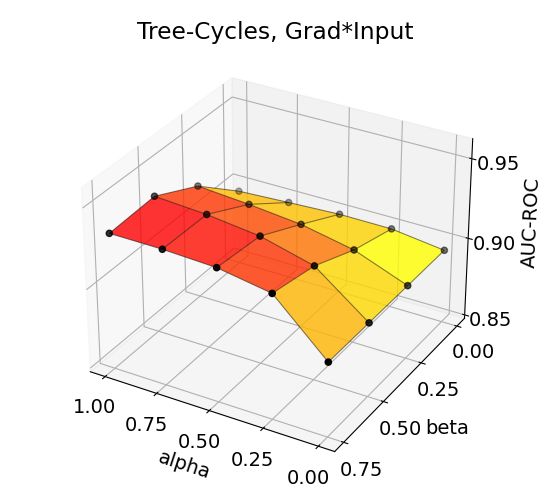
4.1   Auxiliary explanation acquisition

The first step of the auxiliary explanation acquisition is the selection of assistant nodes from which to
collect explanations. Selecting an appropriate set of assistant nodes Va is crucial for obtaining helpful
auxiliary explanations. To collect meaningful and supportive assistant nodes, we set a distance-based
boundary on the assistant node pool. Distance-based boundary methods measure the number of edges
in the shortest path between a candidate node and a target node to exclude unnecessary nodes for
explanation, which acts as a boundary for sampling assistant nodes from an input graph. We filter the
nodes outside of the k-hop neighborhood of the target node vt when k message-passing layers exist
in a model, instead of considering all nodes within the entire graph. The nodes outside of the k-hop
neighborhood have zero influences on the prediction for the target node, which is the main focus to
be explained, and thus, is considered to be inappropriate for collecting auxiliary explanations for the
target.
When the assistant nodes are prepared, the explainability technique is applied to generate explanations
for the assistant nodes. It should be noted that explaining the assistant nodes is not perfectly identical
to explaining the target node. Given the explainability technique E XPLAIN, target node vt , and
model prediction yt , the logit y c with the most probable class label c, is utilized to explain the target
node. On the other hand, to explain the assistant node va , the logit yac with the same class label c is
employed, regardless of the predicted class for va :
                                                                                                c
                S(vt ) = E XPLAIN (G, vt ) = E XPLAIN (G, ytc ) ,              ytc = Φ (G, vt )             (1)
                                                                                                    c
                S(va ) = E XPLAIN (G, va ) = E XPLAIN (G,            yac ) ,   yac   = Φ (G, va )           (2)
                                                                                                        c
where E XPLAIN is the explainability technique, c is the true class label for vt , and Φ(G, v) is the
logit for model prediction on v with class c. Using the logit with the same class label for explanation
allows sharing explanations across the nodes.

4.2   Explanation aggregation

With the explanations S(vt ) and {S(va ) | va ∈ Va } that are obtained from the target node vt and
assistant node Va , respectively, a summarized explanation S̄(vt ) is calculated as a final explanation
for the target node vt . When aggregating explanations, the choice of aggregation formula can be
diverse. Here, we hypothesize that the auxiliary explanation obtained from the important assistant
node would be more influential and supportive for the target explanation. In detail, we assign a
high weight to the auxiliary explanation generated by the assistant node that had high importance
in the original target explanation, whereas a low weight is assigned to the auxiliary explanation
from the low-importance assistant node. To model the importance-based weighted summation of
auxiliary explanations, we design our aggregation formula to incorporate two coefficients, α and
β, for modeling the significance of auxiliary explanations and exponentially decaying weight with
respect to the importance ranking of assistant nodes. It is possible to use an arbitrary decaying series
to model the decaying weights. We chose a simple, exponentially decaying series for our study to
examine the efficacy of our system (Equation 3).
                                                        |Va |
                                                        X
                                 S̄(vt ) = S(vt ) + α           β r−1 S(v (r) )                             (3)
                                                        r=1

where |Va | is the number of assistant nodes within the assistant node set, v (r) is the rth assistant node
by the decreasing importance score from the target explanation S(vt ), α is the weight coefficient for
auxiliary explanations in range [0, 1], and β is the decay coefficient in range [0, 1) for addressing
auxiliary explanations with low importance scores. The coefficients α and β are shared within a
graph in which identical values are applied to explain all nodes for a given dataset and explainability
technique combination.
The equation can be simplified in particular combinations of α and β; for example, when α is set to
0, the equation disregards all auxiliary explanations similar to common explanation techniques. If
α > 0 and β → 1, the equation models equivalent handling of auxiliary explanations regardless of
the importance of its origin node:
                                                        X
                                   S̄(vt ) ≈ S(vt ) + α     S(va )                              (4)
                                                           va ∈Va

                                                    4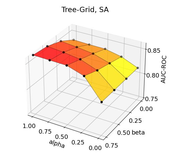
Algorithm 1 Shapening Explanations using S EEN
 1: procedure S EEN(Graph G = (V, E), target node vt , explainability technique E XPLAIN, number
      of message-passing layers k, coefficients α and β)
 2:    S(vt ) ← E XPLAIN(G, vt )                                                             . Eq. (1)
 3:    Update S̄(vt ) ← S(vt )
 4:    for each va ∈ V do
 5:        if 0 < D ISTANCE(vt , va ) ≤ k then                            . Distance-based boundary
 6:             r ← R ANK(S(vt ), va )                                      . Rank va by sa ∈ S(vt )
 7:             S(va ) ← E XPLAIN(G, va )                                                  . Eq. (2)
 8:             Update S̄(vt ) ← S̄(vt ) + αβ r−1 S(va )                                   . Eq. (3)
 9:        end if
10:    end for
11: end procedure

4.3    Motivation

The intuition behind the collection of auxiliary explanations of S EEN is to gather information across
the receptive fields of GNNs and earn a (locally) shared explanation. Each message-passing layer of
a GNN transfers information from each node to their neighboring nodes, expanding the receptive
field by one hop. With a k-layered GNN, the receptive field corresponds to the k-hop neighborhood
of the prediction target. Because all nodes within the k-hop contribute to the prediction for a target
node, a bounding assistant node pool is needed in the k-hop neighborhood.
Within the receptive field, S EEN aggregates auxiliary explanations in order of their node impor-
tance from the target explanation S(vt ) to refine explanations through overlaying neighborhood
explanations. In terms of a community detection problem that predicts each node to certain classes,
predicting the class for a node near the community boundary would suffer from ambiguity of the
boundary criteria. Neighborhoods of the node that partially share the criteria can help to sharpen
the boundary to decide to which community the target belongs, due to the local proximity between
the target node and neighborhoods. Accumulating and overlaying the boundary criteria within the
local neighborhoods would refine the original criteria and can be extended to sharpening explanations
for the predictions. Based on this idea, we conjecture that the explanation could be sharpened by
accumulation of auxiliary explanations from neighboring nodes that have a nonzero contribution to
the target prediction.

5     Experiments

To assess the effectiveness of our conjecture, we conducted a series of experiments on explaining
predictions from graph neural networks in node classification tasks. First, we describe datasets
(Section 5.1) and the model employed for training and explaining graph neural networks (Section 5.2).
Second we present explainability techniques to be examined (Section 5.3) and evaluation criteria
(Section 5.4) for measuring the performance of S EEN. Through qualitative and quantitative analyses,
we demonstrate that our method can improve the explanation accuracy to a maximum of 12.71%
in the best performing case, without losing accuracy in the least-performing cases. Screening the
aggregation coefficients α and β shows that our conjecture, which seeks sharpening explanations
through accumulation of explanations from neighborhoods, is valid. Moreover, the screening process
also reveals that a certain trend exists for coefficient-performance relation and assigning appropriate
values is highly important for maximizing the sharpening effect of S EEN.

5.1    Datasets

We utilize four widely used public synthetic datasets for evaluating explainability techniques on
node classification tasks constructed by Ying et al. [12]: BA-Shapes, BA-Community, Tree-Cycles,
and Tree-Grid. All datasets pursue the classification of each node into their role in attached motifs,
including not-participating positions. The BA-Shapes dataset contains Barabasi-Albert (BA) graphs
decorated with house-structured motifs in random positions. Nodes are numbered 0 to 3 for not-
participating, located on the top, middle, and bottom of the motif. The BA-Community dataset is a

                                                  5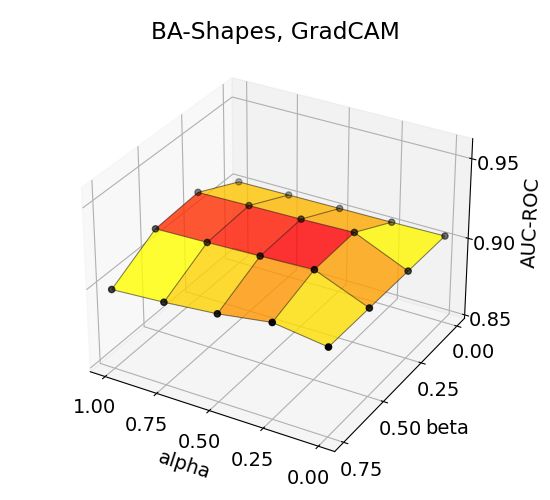
set of graphs made by a combination of two graphs from the BA-Shapes dataset with doubled node
classes. Each node in the BA-Shapes subgraph is given with the node feature based on its community
membership. The Tree-Cycles dataset contains an 8-level tree with randomly attached hexagonal
cycle motifs. The task is to binary classify each node regardless of whether it participates in cycle
motifs. The Tree-Grid dataset is a replacement of the cycle motifs into 3-by-3 grid motifs from the
Tree-Cycles dataset. No node features are provided for any datasets, except for the BA-Community
dataset. Data splits for each dataset are taken from the code by Luo et al. [13], which divides the
dataset into 80%, 10%, and 10% portions for training, validation, and testing, respectively.

5.2   Model

All of experiments are conducted with a GCN model [2] for node classification with three message-
passing layers. The GCN model is trained with cross-entropy loss for ten different random seed
values to generate ten individually trained models. The trained models are then frozen and shared by
all explanation experiments. Detailed architecture, training hyperparameters, and averaged model
accuracies for the GCN model are provided in Appendix.

5.3   Explainability methods

To evaluate the explanation sharpening performance of S EEN, we adopt the following three GNN
explainability techniques, which are compatible with explaining node classification tasks: sensitivity
analysis (SA) [9, 11, 19], Grad*Input [27, 33], and GradCAM [9, 21, 33]. Explainability methods
based on gradients and features are particularly well-suited for S EEN due to their fast and no-
training-required characteristics. However, we would like to emphasize that S EEN is not associated
with specific techniques for the enhancement target. When calculating gradients was required for
explaining assistant nodes, we measured te gradient of the logit that belongs to the same class as the
target node is predicted to be, as previously mentioned in Equation 2 in Section 4.1.

Sensitivity Analysis We utilize the basic SA method [19], which calculates the gradient of the
prediction with respect to the features and generates scores by taking the absolute value of the
gradient. SA measures the influence of each input value on the final prediction through the gradient
and assumes that higher absolute gradient values indicate the higher importance. Due to its simplicity,
transferring SA to GNNs can be easily done by calculating the gradient with respect to the node
features instead of pixels [9, 11]. It is possible to apply SA on explaining predictions with scoring
both nodes and feature elements, we focus on scoring each node in this paper.

Grad*Input Similar to the SA on GNNs, Grad*Input [27, 33] on GNNs calculates the explanation
through element-wise multiplication of node features and their gradient over the prediction and the
consequent summation over the feature dimension to generate node scores. Compared to the SA, the
gradient from Grad*Input is directly multiplied to the input, and the absolute value is obtained after
the multiplication.

GradCAM GradCAM [21] generalizes the class activation map (CAM) method [20], which
requires a global average pooling layer in the model architecture, with gradients from each layer.
Node representations from intermediate message-passing layers are element-wisely multiplied with
their gradients over prediction and summed into a single score value. A detailed formulation for
applying GradCAM on GNNs varies from reported papers [9, 33], such as the selection of the target
layer, averaging the gradients node-wisely or taking the absolute value; we take an approach similar
to the GradCAM(all) method applied by Sanchez-Lengeling et al. [33], which multiplies the gradient
and features element-wisely and averages the scores from each layer. Absolute values are obtained at
the final stage of the explanation.

5.4   Evaluation

We perform experiments with all combinations of the aforementioned four datasets and three explain-
ability techniques to quantify the explanation sharpening ability of S EEN. Since the ground-truth
explanation (the binary labels whether each node is motif-participating) is available for the datasets
due to their synthetic nature, we measure the area under the receiver operation characteristic curve
(AUC-ROC) between the ground-truth and the obtained explanations, similar to Ying et al. [12] and

                                                  6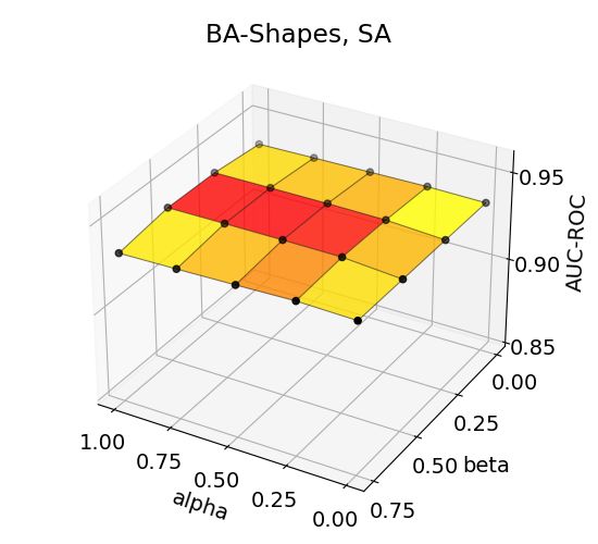
Sanchez-Lengeling et al. [33]. Based on the measure, we calculate the difference in the explanation
accuracy with or without S EEN on each combination.
It should be noted that a modification is made on the test set of the datasets when compared to the
original protocol by Ying et al. Originally, an evaluation is conducted only for the set of selected
nodes, one node per one motif. Instead, we perform an evaluation for all nodes participating in the
motifs instead of using the selected node set. For example, all five nodes that construct a house-
structured motif in the BA datasets are accounted for in the evaluation target, rather than utilizing
only the left top node of each house-structured motif.

5.5   Results

Evaluation on explanation sharpening Table 1 shows the change in the explanation accuracy
when S EEN is applied to different pairs of datasets and explainability techniques. The significance of
the difference is analyzed with a one-sided paired t-test or a one-sided Wilcoxon signed-rank test
based on the normality test results. Statistical analyses show that S EEN significantly increases the
accuracy on providing motif-participating nodes as an explanation for the predictions, to a maximum
of 12.71% on the BA-Community dataset. In the least-performing cases, the measured explanation
accuracy is equivalent to the original explanation when statistically analyzed. An extended table with
the standard deviations, p-values, and aggregation coefficients is included in Appendix. These results
indicate that S EEN successfully generates a sharpened explanation with higher accuracies through
collecting supportive auxiliary explanations around the target node.

Table 1: Explanation accuracies (AUC-ROC) before and after applying S EEN. The best performing
accuracies among the combinations of α and β are listed for each dataset and explainability technique.
Differences that are not significant by statistical analyses are marked as n.s.
      Explainability Methods      BA-Shapes      BA-Community         Tree-Cycles     Tree-Grid
      SA                             0.935             0.625             0.886           0.814
      SA + S EEN                     0.938             0.637             0.900           0.866
      Improvement                     n.s.             1.85%              n.s.            n.s.
      Grad*Input                     0.925             0.614             0.894           0.722
      Grad*Input + S EEN             0.936             0.618             0.934           0.800
      Improvement                    1.18%             0.52%             4.46%          10.77%
      GradCAM                        0.904             0.573             0.750           0.757
      GradCAM + S EEN                0.918             0.645             0.756           0.785
      Improvement                    1.62%            12.71%              n.s.            n.s.

Analysis on explanation aggregation coefficients Our aggregation design leverages the amount
of auxiliary explanation to be incorporated with the target explanation through two coefficients, α and
β. To understand the performance trend with respect to the coefficients, we perform a grid scan over
the coefficients by a 0.25 increment within [0, 1] for α and [0, 1) for β and measure the explanation
accuracy. The β = 1 configurations are additionally tested but excluded from the results for visual
clarity due to the dramatic decrease in performance compared to the other configurations (data not
shown). The low performance for β = 1 suggests that equivalently taking into account all auxiliary
explanations is not beneficial for sharpening the explanation. Thus, assigning an appropriate series of
decreasing weights when aggregating explanations is necessary for accuracy enhancement.
The accuracy trends for BA-Community and Tree-Grid datasets (Figure 2) show that maximum
performance is achieved in high α and medium-to-high β, indicating the helpfulness of auxiliary
explanations toward the target explanation. The performance trends for all combinations are depicted
in Appendix. Moreover, a similar performance trend is observed in other datasets, proving that our
hypothesis on sharpening an explanation with importance-ranked neighborhood explanations. Note
that accuracies change even up to 0.1 in the AUC-ROC upon the choice of α and β. We recommend
conducting a parameter scan to obtain a higher performance increase with S EEN.
An interesting observation is that GradCAM shows distinctive performance patterns and that the
maximum performance is obtained in low α and medium β, compared to other methods that generally

                                                  7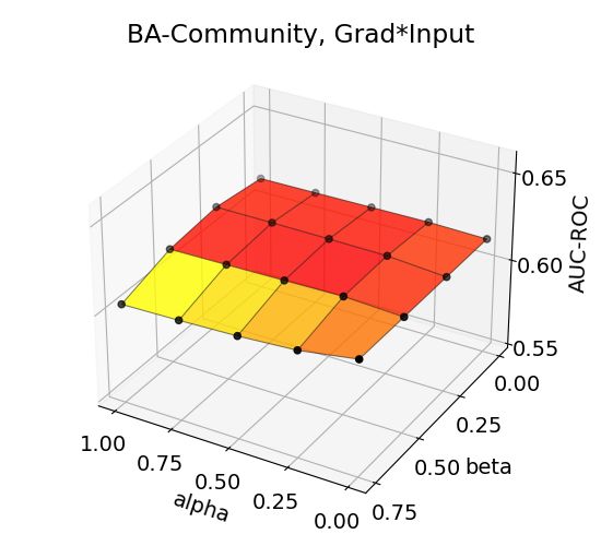
reach their maximum at high α and high β. We assume that the difference may be attributable to the
difference in handling explanation-hop relations; GradCAM collects explanations from each and all
message-passing layers/hops of GNN, whereas SA and Grad*Input generate explanation within the
input layer, which is basically 0-hop. The performances for GradCAM with α = 0.25 are still shown
to be higher than those with α = 0, suggesting that auxiliary explanations are supportive in all cases.

    (a) BA-Community, SA            (b) BA-Community, Grad*Input        (c) BA-Community, GradCAM

       (d) Tree-Grid, SA               (e) Tree-Grid, Grad*Input           (f) Tree-Grid, GradCAM
Figure 2: Effects of aggregation coefficients on explanation accuracy for BA-Community and Tree-
Grid datasets. The results for the remaining combinations are listed in the Appendix.

6   Limitations
Before finishing, we describe limitations of our work in three aspects: applicable task, dataset, and
explainability method. Fundamental mechanism of S EEN, which acquires additional explanations
from assistant nodes, limits the applicable scope of S EEN to node-level prediction tasks. The graph-
level prediction tasks are not applicable due to the inability of collecting multiple explanations from
neighborhoods. Next, our experiments are conducted with synthetic datasets. It is worth noting that
"correct" explanations on graphs are considered to be more ambiguous compared to images, that
synthetic dataset with ground-truth explanation is necessary for evalaution. Still, applying S EEN on
real-world data may have different aspects and trends from the empirical results presented in this
paper. Finally, the employed explainability methods in our paper are gradient/feature-based methods.
Recent methods involving graph masks are compatible with S EEN, but investigation on assigning
importance-based weights is necessary due to their edge-based scoring mechanism.

7   Conclusion
In this paper, we propose S EEN, an explanation sharpening method using auxiliary explanations
obtained from neighboring nodes. Through aggregation of auxiliary explanations with importance-
based weights, S EEN generates a neighborhood-shared explanation without a modification of the
data or an extra model training for explanation enhancement. Our experiments show that our simple
method can significantly increase the explanation accuracy, in conjunction with the open choice for
the explainability technique. Moreover, accuracy trends of aggregation coefficients confirm that
our strategy to assign high weights on important nodes is suitable for sharpening explanations by
overlaying auxiliary explanations. We expect that our approach would improve the reliability of GNN
predictions and expand the scope of the explainability technique to various GNN applications.

                                                  8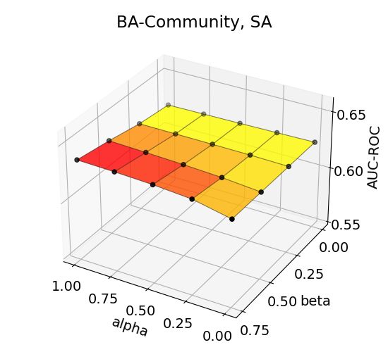
Broader Impact
Explaining predictions from graph neural networks are becoming more important, with the expanding
use of the GNN model on graph-structured data. Explainability techniques help users to obtain
hints on why such a prediction is made and allow them to revise the model. This paper proposed
an explanation sharpening method that utilizes auxiliary explanations from neighborhoods and
demonstrated the efficacy on increasing the explanation accuracy. Moreover, the post hoc attachable
manner of the method allows application on numerous situations across data and explainability
techniques. Because there is still no perfect explainability method, a careful interpretation of
explanations would be required for real-world data. Overreliance on the explanations may mislead
decisions and be vulnerable to biases. We hope that our work will benefit GNN applications by
improving the transparency of GNN models, which is highly important for critical uses requiring
credibility and fairness, such as drug discovery, medical care, and social communication.

Acknowledgments and Disclosure of Funding
We thank Taehee Lee for his helpful comments. Funding in direct support of this work was obtained
from Samsung SDS.

References
 [1] William L Hamilton, Rex Ying, and Jure Leskovec. Inductive representation learning on large
     graphs. In NeurIPS, pages 1025–1035, 2017.

 [2] Thomas N Kipf and Max Welling. Semi-supervised classification with graph convolutional
     networks. In ICLR, 2017.

 [3] Dongkuan Xu, Wei Cheng, Dongsheng Luo, Xiao Liu, and Xiang Zhang. Spatio-temporal
     attentive rnn for node classification in temporal attributed graphs. In IJCAI, pages 3947–3953,
     2019.

 [4] Joan Bruna, Wojciech Zaremba, Arthur Szlam, and Yann LeCun. Spectral networks and deep
     locally connected networks on graphs. In ICLR, 2014.

 [5] Michaël Defferrard, Xavier Bresson, and Pierre Vandergheynst. Convolutional neural networks
     on graphs with fast localized spectral filtering. In NeurIPS, pages 3844–3852, 2016.

 [6] Petar Veličković, Guillem Cucurull, Arantxa Casanova, Adriana Romero, Pietro Lio, and Yoshua
     Bengio. Graph attention networks. In ICLR, 2018.

 [7] Justin Gilmer, Samuel S Schoenholz, Patrick F Riley, Oriol Vinyals, and George E Dahl. Neural
     message passing for quantum chemistry. In ICML, pages 1263–1272, 2017.

 [8] Keyulu Xu, Weihua Hu, Jure Leskovec, and Stefanie Jegelka. How powerful are graph neural
     networks? In ICLR, 2019.

 [9] Phillip E Pope, Soheil Kolouri, Mohammad Rostami, Charles E Martin, and Heiko Hoffmann.
     Explainability methods for graph convolutional neural networks. In CVPR, pages 10772–10781,
     2019.

[10] Hao Yuan, Haiyang Yu, Shurui Gui, and Shuiwang Ji. Explainability in graph neural networks:
     A taxonomic survey. arXiv preprint arXiv:2012.15445, 2021.

[11] Federico Baldassarre and Hossein Azizpour. Explainability techniques for graph convolutional
     networks. In ICML Workshop on Learning and Reasoning with Graph-Structured Representa-
     tions, 2019.

[12] Rex Ying, Dylan Bourgeois, Jiaxuan You, Marinka Zitnik, and Jure Leskovec. Gnnexplainer:
     Generating explanations for graph neural networks. In NeurIPS, 2019.

                                                 9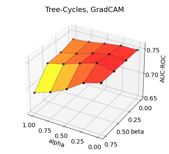
[13] Dongsheng Luo, Wei Cheng, Dongkuan Xu, Wenchao Yu, Bo Zong, Haifeng Chen, and Xiang
     Zhang. Parameterized explainer for graph neural network. In NeurIPS, pages 19620–19631,
     2020.
[14] Michael Sejr Schlichtkrull, Nicola De Cao, and Ivan Titov. Interpreting graph neural networks
     for nlp with differentiable edge masking. arXiv preprint arXiv:2010.00577, 2020.
[15] Minh Vu and My T Thai. Pgm-explainer: Probabilistic graphical model explanations for graph
     neural networks. In NeurIPS, pages 12225–12235, 2020.
[16] David Duvenaud, Dougal Maclaurin, Jorge Aguilera-Iparraguirre, Rafael Gómez-Bombarelli,
     Timothy Hirzel, Alán Aspuru-Guzik, and Ryan P Adams. Convolutional networks on graphs
     for learning molecular fingerprints. In NeurIPS, pages 2224–2232, 2015.
[17] Muhan Zhang and Yixin Chen. Link prediction based on graph neural networks. In NeurIPS,
     pages 5171–5181, 2018.
[18] Seyed Mehran Kazemi and David Poole. Simple embedding for link prediction in knowledge
     graphs. In NeurIPS, pages 4289–4300, 2018.
[19] Karen Simonyan, Andrea Vedaldi, and Andrew Zisserman. Deep inside convolutional networks:
     Visualising image classification models and saliency maps. arXiv preprint arXiv:1312.6034,
     2013.
[20] Bolei Zhou, Aditya Khosla, Agata Lapedriza, Aude Oliva, and Antonio Torralba. Learning deep
     features for discriminative localization. In CVPR, pages 2921–2929, 2016.
[21] Ramprasaath R Selvaraju, Michael Cogswell, Abhishek Das, Ramakrishna Vedantam, Devi
     Parikh, and Dhruv Batra. Grad-cam: Visual explanations from deep networks via gradient-based
     localization. In ICCV, pages 618–626, 2017.
[22] Aditya Chattopadhay, Anirban Sarkar, Prantik Howlader, and Vineeth N Balasubramanian.
     Grad-cam++: Generalized gradient-based visual explanations for deep convolutional networks.
     In WACV, pages 839–847, 2018.
[23] Luisa M Zintgraf, Taco S Cohen, Tameem Adel, and Max Welling. Visualizing deep neural
     network decisions: Prediction difference analysis. In ICLR, 2017.
[24] Ruth C Fong and Andrea Vedaldi. Interpretable explanations of black boxes by meaningful
     perturbation. In ICCV, pages 3429–3437, 2017.
[25] Ruth Fong, Mandela Patrick, and Andrea Vedaldi. Understanding deep networks via extremal
     perturbations and smooth masks. In ICCV, pages 2950–2958, 2019.
[26] Sebastian Bach, Alexander Binder, Grégoire Montavon, Frederick Klauschen, Klaus-Robert
     Müller, and Wojciech Samek. On pixel-wise explanations for non-linear classifier decisions by
     layer-wise relevance propagation. PLOS ONE, 10(7):1–46, 2015.
[27] Avanti Shrikumar, Peyton Greenside, and Anshul Kundaje. Learning important features through
     propagating activation differences. In ICML, pages 3145–3153, 2017.
[28] Thorben Funke, Megha Khosla, and Avishek Anand. Hard masking for explaining graph neural
     networks, 2021. URL https://openreview.net/forum?id=uDN8pRAdsoC.
[29] Xiang Wang, Yingxin Wu, An Zhang, Xiangnan He, and Tat-seng Chua. Causal screen-
     ing to interpret graph neural networks, 2021. URL https://openreview.net/forum?id=
     nzKv5vxZfge.
[30] Thomas Schnake, Oliver Eberle, Jonas Lederer, Shinichi Nakajima, Kristof T Schütt, Klaus-
     Robert Müller, and Grégoire Montavon. Higher-order explanations of graph neural networks
     via relevant walks. arXiv preprint arXiv:2006.03589, 2020.
[31] Daniel Smilkov, Nikhil Thorat, Been Kim, Fernanda Viégas, and Martin Wattenberg. Smooth-
     grad: removing noise by adding noise. arXiv preprint arXiv:1706.03825, 2017.

                                               10
[32] Youngrock Oh, Hyungsik Jung, Jeonghyung Park, and Min Soo Kim. Evet: Enhancing visual
explanations of deep neural networks using image transformations. In WACV, pages 3579–3587,
2021.
[33] Benjamin Sanchez-Lengeling, Jennifer Wei, Brian Lee, Emily Reif, Peter Wang, Wesley Wei
Qian, Kevin McCloskey, Lucy Colwell, and Alexander Wiltschko. Evaluating attribution for
graph neural networks. In NeurIPS, pages 5898–5910, 2020.
[34] Adam Paszke, Sam Gross, Francisco Massa, Adam Lerer, James Bradbury, Gregory Chanan,
Trevor Killeen, Zeming Lin, Natalia Gimelshein, Luca Antiga, Alban Desmaison, Andreas
Kopf, Edward Yang, Zachary DeVito, Martin Raison, Alykhan Tejani, Sasank Chilamkurthy,
Benoit Steiner, Lu Fang, Junjie Bai, and Soumith Chintala. Pytorch: An imperative style,
high-performance deep learning library. In NeurIPS, pages 8024–8035, 2019.
[35] Matthias Fey and Jan E Lenssen. Fast graph representation learning with pytorch geometric. In
ICLR Workshop on Representation Learning on Graphs and Manifolds, 2019.
Checklist
1. For all authors...
(a) Do the main claims made in the abstract and introduction accurately reflect the paper’s
contributions and scope? [Yes] Our claims are described in Introduction section and
summarized in the abstract.
(b) Did you describe the limitations of your work? [Yes] Limitations of our work in three
aspects are listed in Limitation section.
(c) Did you discuss any potential negative societal impacts of your work? [Yes] Discussion
on the potential negative impacts are described in Broader Impact section.
(d) Have you read the ethics review guidelines and ensured that your paper conforms to
them? [Yes] Authors have read and checked the paper based on the ethics review
guidelines.
2. If you are including theoretical results...
(a) Did you state the full set of assumptions of all theoretical results? [Yes] We describe
our conjecture on aggregating explanations in Section 4.3.
(b) Did you include complete proofs of all theoretical results? [N/A] We do not include
theoretical results require proofs.
3. If you ran experiments...
(a) Did you include the code, data, and instructions needed to reproduce the main ex-
perimental results (either in the supplemental material or as a URL)? [Yes] Detailed
experimental information are listed either in Section 5 and Appendix. Code for the
experiments are to be made public in near future.
(b) Did you specify all the training details (e.g., data splits, hyperparameters, how they
were chosen)? [Yes] See Section 5.1 and Appendix for details on data. Training
hyperparameters are listed in Appendix. Detailed model information can be found in
Section 5.2 and Appendix.
(c) Did you report error bars (e.g., with respect to the random seed after running experi-
ments multiple times)? [Yes] For the standard deviations by the ten-fold experiments,
see extended table in Appendix.
(d) Did you include the total amount of compute and the type of resources used (e.g., type
of GPUs, internal cluster, or cloud provider)? [Yes] Hardware details for experiments
are listed in Appendix.
4. If you are using existing assets (e.g., code, data, models) or curating/releasing new assets...
(a) If your work uses existing assets, did you cite the creators? [Yes] We adopt synthetic
datasets constructed by Ying et al. and data splits from Luo et al.. Citations are added
at their occurance (see Section 5.1 and Appendix).
(b) Did you mention the license of the assets? [Yes] We mention the license of used
datasets in Appedix with corresponding citation.
11(c) Did you include any new assets either in the supplemental material or as a URL? [N/A]
We do not include new assets in our experiments.
(d) Did you discuss whether and how consent was obtained from people whose data you’re
using/curating? [Yes] The dataset is open publically via official Github repository of
Ying et al. [12] under Apache License 2.0. We cite the dataset and the constructors in
Section 5.1 and Appendix.
(e) Did you discuss whether the data you are using/curating contains personally identifiable
information or offensive content? [N/A] Data used in our research are synthetic and
abstract graph datasets, which do not include personal information.
5. If you used crowdsourcing or conducted research with human subjects...
(a) Did you include the full text of instructions given to participants and screenshots,
if applicable? [N/A] Our work does not include experiments/research with human
subjects.
(b) Did you describe any potential participant risks, with links to Institutional Review Board
(IRB) approvals, if applicable? [N/A] Our work does not include experiments/research
requiring IRB approvals.
(c) Did you include the estimated hourly wage paid to participants and the total amount
spent on participant compensation? [N/A] Our work does not include experi-
ments/research with human subjects.
12A Experimental details
A.1 Hardware and environment
Experiments are conducted on a Ubuntu 16.04 server with four RTX Titan GPUs with 24GB memory
each. Python 3.6.10 environment with CUDA version 10.1 and NVIDIA driver version 418.39 is used.
All models are implemented with Pytorch [34] version 1.6.0 and Pytorch Geometric [35] version
1.6.1.
A.2 Model architecture and training
We use basic graph convolutional network (GCN) [2] model for all experiments. Three-layered GCN
model with node feature concatenation and fully connected layer is used. Entire network architecture
with detailed information is listed in Table 2. Adam optimizer with learning rate 0.001 and L2 weight
decay 0.001 is adopted for all datasets, except for Tree-Grid dataset which utilized 0.002 for the
weight decay. Each model for BA-shapes, Tree-Cycles, and Tree-Grid datasets is trained for 10000
epochs, whereas models for BA-Community dataset are trained for 5000 epochs.
Table 2: Model architecture and hyperparameters.
Layer Type Parameter Value
1 Graph convolution Input shapes #Nodes×#Node features
Output shapes #Nodes×20
Activation ReLU
2 Graph convolution Input shapes #Nodes×20
Output shapes #Nodes×20
Activation ReLU
3 Graph convolution Input shapes #Nodes×20
Output shapes #Nodes×20
Activation ReLU
4 Concatenation Input shapes Three #Nodes×20 from Layer 1, 2, 3
Output shapes #Nodes×60
5 Fully connected Input shapes #Nodes×60
Output shapes #Nodes×#Classes
Activation None
A.3 Dataset
Datasets are taken from GNNExplainer paper [12] under Apache License 2.0. Dataset split is taken
from the PGExplainer code by Luo et al. [13], which splits train/validation/test sets by 80/10/10%.
Averaged prediction accuracies with standard deviations for the trained models are listed in Table 3.
Accuracies for the datasets are considered to be high enough for explanation experiments and no
further hyperparameter scan is conducted.
Table 3: Prediction accuracies (AUC-ROC) for the trained models.
Data split BA-Shapes BA-Community Tree-Cycles Tree-Grid
Training 0.966±0.029 0.999±0.000 0.944±0.005 0.902±0.005
Validation 0.973±0.021 0.794±0.023 0.951±0.005 0.935±0.023
Test 0.964±0.038 0.805±0.024 0.947±0.011 0.934±0.011
13B Supplementary results
B.1 Explanation accuracy
All explanation-generating experiments are conducted in ten-fold with the ten aforementioned trained
models for each dataset. Extended accuracy table with standard deviations and p-values corresponding
to the Table 1 is shown in Table 4. For statistical analysis, each result is first assessed with normality
test to check their distribution. For pairs with at least one p < 0.05 in normality test, one-sided
Wilcoxon signed-rank test is used for analysis. For the rest, one-sided Student’s T-test is used.
Table 4: Explanation accuracies (AUC-ROC) before and after applying S EEN with standard deviations,
p-values, and their best performing α and β values.
Explainer BA-Shapes BA-Community Tree-Cycles Tree-Grid
SA 0.935±0.009 0.625±0.020 0.886±0.050 0.814±0.112
SA + S EEN 0.938±0.005 0.637±0.018 0.900±0.035 0.866±0.136
p-value 6.5×10⁻² 9.4×10⁻³ 1.4×10⁻¹ 5.2×10⁻²
(α, β) (0.5, 0.5) (1.0, 0.75) (1.0, 0.5) (1.0, 0.75)
Grad*Input 0.925±0.011 0.614±0.015 0.894±0.051 0.722±0.143
Grad*Input + S EEN 0.936±0.056 0.718±0.015 0.934±0.033 0.800±0.124
p-value 9.8×10⁻⁴ 1.5×10⁻² 9.8×10⁻⁴ 2.1×10⁻²
(α, β) (1.0, 0.5) (1.0, 0.25) (1.0, 0.5) (1.0, 0.5)
GradCAM 0.904±0.055 0.573±0.001 0.750±0.041 0.757±0.029
GradCAM + S EEN 0.918±0.000 0.645±0.024 0.756±0.071 0.785±0.060
p-value 1.6×10⁻⁴ 2.8×10⁻⁶ 1.4×10⁻¹ 5.2×10⁻²
(α, β) (0.25, 0.25) (1.0, 0.25) (0.25, 0.5) (0.25, 0.5)
B.2 Aggregation coefficients
Performance scan over aggregation coefficients is conducted within [0, 1] for α and [0, 1) for β with
0.25-increament. Note that performances for varying β with α = 0 are identical, depicted as the right
bottom line of each plot in Figure 3.
14Figure 3: Effects of aggregation coefficients on explanation accuracy for BA-Shapes, BA-Community,
Tree-Cycles, and Tree-Grid datasets.
15You can also read