A route pruning algorithm for an automated geographic location graph construction
←
→
Page content transcription
If your browser does not render page correctly, please read the page content below
www.nature.com/scientificreports
OPEN A route pruning algorithm
for an automated geographic
location graph construction
Christoph Schweimer1, Bernhard C. Geiger1*, Meizhu Wang1, Sergiy Gogolenko2,
Imran Mahmood3, Alireza Jahani3, Diana Suleimenova3* & Derek Groen3,4
Automated construction of location graphs is instrumental but challenging, particularly in logistics
optimisation problems and agent-based movement simulations. Hence, we propose an algorithm for
automated construction of location graphs, in which vertices correspond to geographic locations of
interest and edges to direct travelling routes between them. Our approach involves two steps. In the
first step, we use a routing service to compute distances between all pairs of L locations, resulting in a
complete graph. In the second step, we prune this graph by removing edges corresponding to indirect
routes, identified using the triangle inequality. The computational complexity of this second step is
O(L3 ), which enables the computation of location graphs for all towns and cities on the road network
of an entire continent. To illustrate the utility of our algorithm in an application, we constructed
location graphs for four regions of different size and road infrastructures and compared them to
manually created ground truths. Our algorithm simultaneously achieved precision and recall values
around 0.9 for a wide range of the single hyperparameter, suggesting that it is a valid approach to
create large location graphs for which a manual creation is infeasible.
Geographic information systems (GIS) and web mapping have evolved over the past three decades as techno-
logical advances enable the developments in geospatial data and mapping u sage1. Consequently, web mapping
services, such as Google Maps, Bing Maps and OpenStreetMap (OSM), have emerged with various functionalities
to inspect, visualise, analyse and model geospatial information. These commonly known services are available
and accessible by everyone through interactive and visual interfaces, as well as provide an interface to download
geographic information, including lists of cities or other points-of-interest within a geographic region, and routes
between pairs of locations (if the service also provides routing capabilities).
However, these interfaces have functional limitations, which do not allow the automatic generation of highly
customised geographic information. In this work, we consider a relevant subclass of such customised geographic
information: location graphs, in which locations of interest are connected by edges if there exists a direct route
between them. Such location graphs are a prerequisite for many real-life problems, for example, route optimisa-
tion, load optimisation in electrical and transportation networks, and many others. Location graphs are also
needed for agent-based modelling applications such as transportation of g oods2, evacuation m odels3,4, traffic
simulations5, disease transmission6, movement of p eople7, and migration s imulation8.
Previously, these location graphs were created manually. For example, for the migration study of Suleimenova
et al.8, the length of a link (in km) was estimated using the OSM route planner for cars. In cases where obvious
shorter routes are visible, the mapping marker was dragged to force the routing machine to calculate these shorter
routes. Yet, such manual creation of location graphs is a time-consuming and error-prone procedure, and can
only be accomplished for small sets of locations.
We propose an automated approach for the construction of location graphs for given lists of locations. This
approach relies on a two-step procedure. In the first step, we utilise interfaces provided by mapping services,
such as the Open Source Routing Machine (OSRM) from OSM, to compute route distances between all pairs of
locations, essentially corresponding to a fully connected location graph. In the second step, edges are pruned
from this fully connected location graph that correspond to indirect routes, i.e., to routes between two locations
that pass through a third location in the location graph. Since the first step yields only a matrix of distances but
no further information about the routes, finding these indirect routes is nontrivial. We approach this problem
by making use of the triangle inequality: if the route between two locations has a distance similar to the sum of
1
Know-Center GmbH, Graz, Austria. 2High Performance Computing Center Stuttgart, Stuttgart,
Germany. 3Department of Computer Science, Brunel University London, London, UK. 4Centre for Computational
Science, University College London, London, UK. *email: geiger@ieee.org; diana.suleimenova@brunel.ac.uk
Scientific Reports | (2021) 11:11547 | https://doi.org/10.1038/s41598-021-90943-8 1
Vol.:(0123456789)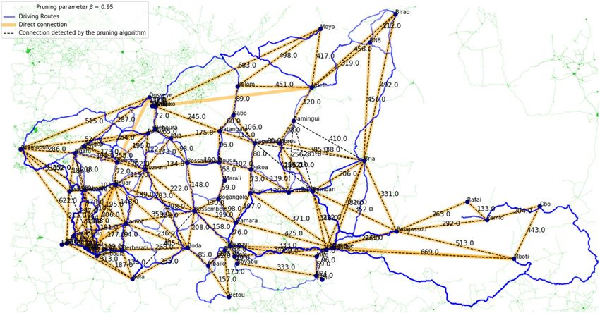
www.nature.com/scientificreports/
distances of routes between these locations and a common third location, then it is probable that the considered
route is indirect. While the first step of our procedure relies on existing algorithms for finding shortest paths
in graphs, the second step presents our first contribution in the area of edge pruning algorithms (see “Related
work” section).
As our second contribution, we add a real-valued parameter β to our pruning algorithm that extends the flex-
ibility of our approach and allows to control the quality of pruning. Specifically, when deciding whether a route
shall be pruned, we compare the route distance between two locations to the sum of distances between these loca-
tions and a third one, multiplied by β. Thus, if β > 1, the resulting pruned graph may not be completely pruned,
but may rather be redundant by retaining edges corresponding to sub-optimal routes (i.e., with longer distances).
If instead 0 < β < 1, then the resulting graph is lossy in the sense that not all shortest paths are retained. Thus,
the parameter β allows trading between the quality (in terms of redundancy and path quality) and complexity
(in terms of edge set size) of the simplified graph. As a consequence, our approach complements and extends the
work of Zhou et al.9,10, who approached graph simplification by pruning a given number of edges such that path
quality is maximised while we control the quality of the lossy pruning by the relaxation parameter 0 < β ≤ 1.
Our third contribution is to validate the applicability of our approach and investigate its limitations by apply-
ing it to four different scenarios. We constructed location graphs for two small regions in Europe and for two
large regions in Africa, respectively, and compared the results to manually created ground truths. In three of the
four regions, we achieved an F1-score (see “Results” section for a definition) exceeding 0.9 for the same value
of the single parameter of our method. We furthermore showed that our approach scales well to larger location
sets, thus enabling the creation of location graphs with tens of thousands of locations. The implementation of
our method is available at https://github.com/djgroen/ExtractMap.
Related work
The shortest path algorithms for route planning can be categorised into static, dynamic, time-dependent, sto-
chastic, parametric, alternative and weighted region shortest-path a lgorithms11,12. These algorithms establish the
algorithmic basis for state-of-the-art route planning engines such as Google Maps, Bing Maps, or OSRM. The
static category includes single-source and all-pairs shortest-path algorithms that differ in terms of a given edge
to other edges or all-pairs to other edges in the graph. One of the most known shortest-path algorithms was
proposed by D ijkstra13. It finds a shortest path between two vertices in a graph. Dijkstra’s algorithm has numer-
ous variations that are commonly applied to speed-up computing and tackle diverse problems of general and
complex graphs11,14. Dynamic algorithms consider insertion and deletion of edges, as well as a computation of
the distances between single-source or all-pairs edges in the graph. Other categories refer to changes over time,
uncertainty in edges, specific parameter values, avoiding given edges and weighted subdivision edges. In this
work, we focus our interest on the category of batched shortest path algorithms which are commonly used for
computing distance matrices in route planning engines12.
State-of-the-art route planning engines implement an API for finding travel distances and journey duration
of fastest routes between all pairs of supplied origins using a given mode of travel. Examples of these include
Distance Matrix Service of Google Maps, Distance Matrix API of Bing Maps, and Table Service of OSRM. Online
routing services impose different constraints on the size and quantity of such API queries. In particular, Bing
API allows up to 2500 origins-destinations pairs, while Google API establishes pricing per origin-destination
pair in the Distance Matrix queries. Moreover, online services usually have a limited uncustomizable set of travel
modes, which prevents tailoring models for speed of traveller movement on different terrains and road types.
Being a free open-source off-line tool, OSRM relaxes these l imitations15.
OSRM implements multilevel Dijkstra’s (MLD) and contraction hierarchies (CH) algorithms for r outing15.
Both methods consist of preprocessing and query phases. The preprocessing phase attempts to annotate and
simplify the complicated route network in order to drastically reduce duration of further shortest-path and
batched shortest-path queries. MLD belongs to the family of separator-based shortest-path t echniques11,12. Con-
ceptually, it differs from the celebrated customizable route planning (CRP) a lgorithm16,17 only by the hierarchical
partitioning approach used in the preprocessing phase: canonical CRP applies patented graph partitioning with
natural cuts (PUNCH) approach, while MLD opts for inertial flow approach18. Contraction hierarchies is a classic
hierarchical shortest-path a lgorithm11,12, widely discussed in the l iterature19,20.
Network simplification by edge pruning emerged in various contexts and has been addressed under differ-
ent names by a number of a uthors9,10,21–25. Specifically, the authors propose and study a generic path-oriented
framework for graph s implification9,10,25. This framework targets to simplify a graph by reducing the number of
edges while preserving the maximum path quality metric for any pair of vertices in the graph. It covers a broad
class of optimisation problems for probabilistic graphs, flow graphs, and distance graphs. Distance graph pruning,
as it is investigated in this work, can be viewed as a special case of the path-oriented graph simplification where
the inverse of the path length serves as a path quality metric. Toivonen et al.25 introduce four generic strategies
for lossless path-oriented graph simplification, where the term lossless in the context of distance graphs implies
that all fastest routes between pairs of locations are preserved in the pruned graph. Later this approach was
extended to a lossy graph pruning with a given number of edges to r emove9,10.
Our pruning approach based on the triangle inequality closely relates to the Static-Triangle strategy from
Toivonen et al.25 which has a time complexity of O (L · R), where L and R are the number of locations and routes
in the original graph, respectively. For general (potentially sparse) graphs, this strategy is sub-optimal in the
sense that the obtained graph may contain redundant routes, and the authors thus also propose an alternative,
optimal strategy (called Iterative-Global) with a higher time complexity of O (R(R + L) log L). However, for a
complete location graph in which route distances satisfy the triangle inequality and ignoring the effect of ties,
the Static-Triangle strategy and our own approach can be shown to be optimal in the sense of eliminating all
Scientific Reports | (2021) 11:11547 | https://doi.org/10.1038/s41598-021-90943-8 2
Vol:.(1234567890)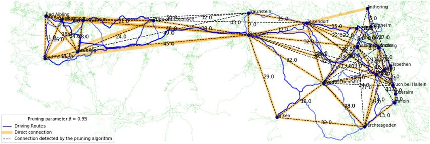
www.nature.com/scientificreports/
redundant routes. In this case, since R = L2, the time complexity of our approach is O (L3 ), which compares
favourably with the time complexity of O (L4 log L) of the optimal Iterative-Global s trategy25. Since the first step
of our two-step approach results with a complete location graph where the route distances satisfy the triangle
inequality, we can reap the benefits of this reduced time complexity without loss of optimality.
Methods
We are given a set of L locations L = {l1 , . . . , lL } in a geographical region. We are interested in a weighted graph
G = (L , E, D) with vertices L, edges E corresponding to direct routes between locations, and edge weights D
corresponding to route distances that keeps only fastest (or shortest) paths between all pairs of vertices from L.
The problem of finding an optimal location graph can be formalised as follows. We assume a weighted,
potentially directed route graph G = (LG , EG ) with LG vertices is given. Each edge e := (u, v) ∈ EG
corresponds to a route connecting two locations u and v from LG and has a positive-valued weight
dG (e) ∈ R+ that corresponds to the route distance between u and v. A path P is a sequence of edges, e.g.
G
P = ((u1 , u2 ), (u2 , u3 ), . . . , (uk−1 , uk )) =: [u1 − u2 − · · · − uk ]. We denote by u1 uk the set of all feasible
paths between u1 and uk in G. The length of the shortest path between u and v is thus defined as
Q(u, v; G) = min dG (e) . (1)
G
P∈u v e∈P
For the given subset of locations L ⊆ LG , our goal is to find a weighted graph G = (L , E) with a minimum
number of edges such that Q(u, v; G ) = Q(u, v; G) for all {u, v} ⊆ L. For the sake of brevity, we limit further
discussion to the undirected graphs. Nevertheless, our approach straightforwardly extends to the directed graphs.
To create the graph G , we propose a two-step procedure. In the first step, we use a routing service to find
route distances between all pairs of locations. Assuming that the distances are symmetric, we terminate with an
undirected fully connected graph G ∗ = (L , [L ]2 , D∗ ), where [L ]2 is the set of two-element subsets of L and
where D∗ = [di,j∗ ] is the matrix of distances between locations with d ∗ = d ∗ ({l , l }). Many of the distances
i,j G i j
computed by the route planner will correspond to indirect routes, as a route between two locations in L may pass
through another location in L. Therefore, in a second step, we use the distance matrix D∗ to identify edges in
G ∗ that correspond to redundant routes, and remove them to obtain G. In this section, we will give an overview
of this two-step procedure.
Step 1: Creating a fully connected graph via route planning. For route planning, we rely on map
data from OSM, together with the C++ routing machine from the OSRM Project (http://project-osrm.org), i.e.,
we work with locally downloaded map data and a C++ wrapper for OSRM, allowing requests for large sets of
locations L. However, any other routing service can be used, including online services for smaller sets of loca-
tions. In our experiments, we obtained pairwise distances between up to L = 18000 locations. The result is a dis-
tance matrix D∗ = [di,j ∗ ], with d ∗ being the distance between locations l and l . If there is no route between l and
i,j i j i
lj , then the respective distance is set to ∞. Throughout this work and in pruning algorithm implementation, we
assume that the matrix D∗ is symmetric and has an all-zero main diagonal, i.e., L(L − 1)/2 degrees of freedom.
Step 2: Algorithm for pruning redundant routes. Of the L(L − 1)/2 route distances obtained in the
previous step, a significant portion will represent indirect routes. For example, suppose that locations l1, l2, and
l3 lie on the same road in a geographical region, with location l2 lying between the other two. The road network
has an edge from l1 to l2 and an edge from l2 to l3, but no direct edge from l1 to l3. Thus, for the construction of
the weight matrix D = [di,j ] in our desired graph G, we need to set d1,3 = d3,1 = ∞ and ensure that the edge
{l1 , l3 } �∈ E.
In order to detect indirect routes, we make use of the following reasoning. If l2 lies on the same road and
between l1 and l3, then one may expect that d1,2 ∗ + d ∗ ≈ d ∗ . In fact, in most cases we will have d ∗ + d ∗ > d ∗ ,
2,3 1,3 1,2 2,3 1,3
because l2 may not lie directly on the route between l1 and l3. At the same time, if l2 lies on the same road and
between l1 and l3, then d1,3 ∗ will be the longest of the three routes, i.e., d ∗ ≥ max{d ∗ , d ∗ }. Thus, if in a triangle of
1,3 1,2 2,3
locations li , lj , and lk with distances di,j
∗ , d ∗ , and d ∗ , the largest distance is larger than the sum of the two smaller
i,k j,k
distances, then it is very likely that the largest distance corresponds to an indirect route, which subsequently is
removed from G ∗ to arrive at G.
Scientific Reports | (2021) 11:11547 | https://doi.org/10.1038/s41598-021-90943-8 3
Vol.:(0123456789)www.nature.com/scientificreports/
The pseudocode in Algorithm 1 summarises these ideas. Note that, by the restriction that i < j < k in line 2,
it only operates on the upper triangle of D∗, since we assume that the matrix D∗ is symmetric. Since the algo-
rithm iterates over all L(L − 1)(L − 2)/6 possible triples of locations, the computational complexity is O (L3 ).
It is important to highlight that Algorithm 1 executes route pruning on a copy of the fully connected graph
(see line 1) while checking the pruning condition on the input graph G ∗ (see line 5). Otherwise, the triplets order
may impact the results of pruning and lead to incorrect conclusions. In particular, Fig. 1 illustrates an example
when the natural lexicographic order of triangle traversal leads to incorrect pruning (Fig. 1b), whereas a slightly
modified order produces the right answer (Fig. 1c).
As can be seen in line 5 of Algorithm 1, we added a parameter β in order to relax the condition posed by
the triangle inequality. A value β < 1 allows removing the longest side of a triangular route even if it is slightly
shorter than the sum of the two remaining routes. This makes sense if three locations lie along a road, but getting
to these locations requires a short detour (e.g. getting off the highway and to the city centre before getting back
on the highway). The larger β , the more conservative is our pruning algorithm. Rather than such a multiplica-
tive relaxation, allowing the largest distance to exceed the sum of the other two distances by some percentage,
an additive relaxation is possible as well, or a combination thereof (e.g. by replacing the condition in line 5 by
∗ > min{d ∗ /β, d ∗ + δ}, where δ is a tunable parameter corresponding to an absolute distance).
s − da,b a,b a,b
The idea of triangular pruning extends naturally to sparse or directed input graphs G ∗ = (L , E ∗ , D∗ ). If the
graph is directed, then E is a subset of L 2 and D∗ need not be symmetric anymore. Such a situation can occur
∗
in cases in which distances between locations depend on the direction between them, e.g. caused by one-way
streets. If the graph is sparse, then E ∗ is a proper subset of L 2 (in the directed case) or [L ]2 (in the undirected
case). This can be caused by prior information on the road network, for example, or by adjustments made in
Step 1 of our approach.
We close this section by showing that Algorithm 1 terminates with a completely pruned graph also in settings
different from the one considered here. For general graphs G ∗, an edge {l1 , lk } is redundant if and only if there is
a path P = [l1 − l2 − · · · − lk ] that is shorter than d1,k
∗ . This consideration is the motivation behind the “Global”
strategies of Toivonen et al.25 Now suppose that the graph G ∗ is complete and satisfies the triangle inequality.
In other words, if P = [l1 − l2 − · · · − lk ] is a path in this graph, then for every vertex lj , j ∈ {2, 3, . . . , k − 1},
we have that the length of P in G ∗ is at least d1,j ∗ + d ∗ (such as in the graph that we obtain in step 1). Then, it
j,k
is apparent that the edge {l1 , lk } is redundant if and only if there is a location lj such that d1,j
∗ + d ∗ < d ∗ . This
j,k 1,k
shows that for these types of graphs the “Triangle” strategies of Toivonen et al.25 and our Algorithm 1 are optimal.
Results
To validate our route pruning approach, understand its limitations and its dependence on the parameter β ,
we tested it in four geographical regions, namely the federal state of Styria in Austria, a region at the German-
Austrian border, the Central African Republic and South Sudan countries.
For Step 1 of our approach we relied on OSM map data downloaded from https://download.geofabrik.de and
applied an offline version of OSRM to compute route distances (shortest driving time) between several location
types, e.g. established cities, small towns and (temporary) refugee camps, in the four considered geographical
regions. We subsequently applied Algorithm 1 for Step 2 to obtain the pruned location graph G.
The accuracy of Algorithm 1 w.r.t. a manually created ground truth of direct driving routes is measured in
terms of Precision, Recall and F1-score. To calculate these three performance indicators, the number of True
Positives (TP), False Positives (FP) and False Negatives (FN) is needed. In our study, a TP is a route that is part
of the ground truth and that is also detected by the pruning algorithm, a FP is a route that is not part of the
ground truth, but is labelled as a direct route by the pruning algorithm, and a FN is a route that is part of the
ground truth, but pruned from the fully connected graph by the algorithm. From these, Precision, Recall, and
F1-score are calculated as follows:
TP TP Precision − Recall
Precision = Recall = F1 - score = 2 ·
TP + FP TP + FN Precision + Recall
In addition to computing quantitative performance measures, we visualised our results in Figs. 2, 3 and 4 (see
also Supplementary Figure S1). These figures were generated using the OSMnx Python package, which is based
etworks26.
on OSM to create, analyse, and visualise street n
Scientific Reports | (2021) 11:11547 | https://doi.org/10.1038/s41598-021-90943-8 4
Vol:.(1234567890)www.nature.com/scientificreports/
Figure 1. Impact of triplets order on pruning results.
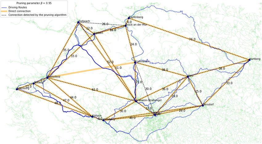
Figure 2. Connections of 15 locations in the federal state of Styria, Austria with β = 0.95.
Creation of the ground truth. We created the ground truth of direct driving connections for each of the
four regions with OSM by inspecting if the fastest route (shortest time) between each location pair is direct. A
connection between two locations is labelled direct if there is no other location on or nearby the fastest route. In
most cases it was clear if a direct driving route between two locations exists, but there are also ambiguous situa-
tions (e.g., route from l1 to l2 is direct, but indirect from l2 to l1) and potential sources of error (e.g., small locations
or refugee camps, especially in large regions, might not be marked explicitly in OSM), such that the creation of
the ground truth was not straightforward (see Supplementary Note 1 for details). Even if the ground truth is
created to the best of our knowledge, some uncertainty remains. Thus, the reported performance measures have
to be interpreted accordingly.
Federal state of Styria, Austria. For the region in the federal state of Styria in Austria, we extracted
towns and cities within a rectangle with the geographic coordinates N47.0 − N47.5 and E14.6 − E16.0 from
OSM. The OSM Overpass A PI27 returned 15 locations within this area, 14 towns and one bigger city, Graz.
Therefore, the fully connected graph of this region contains 105 driving routes connecting the 15 locations. We
obtained 29 direct driving routes between the 15 locations as the ground truth.
Scientific Reports | (2021) 11:11547 | https://doi.org/10.1038/s41598-021-90943-8 5
Vol.:(0123456789)www.nature.com/scientificreports/
Figure 3. Connections of 23 locations in the border region between Germany and Austria with β = 0.95.
Figure 4. Connections of 62 locations in the Central African Republic with β = 0.95.
β Ground truth routes Routes after pruning TP FP FN Precision Recall F1-score
0.900 29 26 26 0 3 1.00 0.90 0.95
0.925 29 27 27 0 2 1.00 0.93 0.96
0.950 29 30 28 2 1 0.93 0.97 0.95
0.975 29 39 29 10 0 0.74 1.00 0.85
Table 1. Results for the triangle inequality pruned graph in Styria, Austria with 15 locations.
The fully connected graph was pruned with Algorithm 1, “Route Pruning for General Undirected Graphs” for
several values of the pruning parameter β. Table 1 contains the results for the pruning parameters 0.9, 0.925, 0.95,
and 0.975. For β ∈ [0.9, 0.95], Precision, Recall and F1-Score are all above 0.9. Figure 2 visualises the results for
β = 0.95 with the established ground truth and pruned connections as well as the suggested fastest driving routes.
For β = 0.95, the pruning algorithm returns 30 direct driving routes between the 15 locations. 28 of the 29
ground truth routes are detected, it prunes one route that is part of the ground truth and declares two routes as
direct connections that are not part of the ground truth. The route [Frohnleiten – Knittelfeld] in the central part
of the region is 69 km long and is pruned from the fully connected graph, but is part of the ground truth. The
Scientific Reports | (2021) 11:11547 | https://doi.org/10.1038/s41598-021-90943-8 6
Vol:.(1234567890)www.nature.com/scientificreports/
β Ground truth routes Routes after pruning TP FP FN Precision Recall F1-score
0.90 57 53 39 14 18 0.73 0.68 0.71
0.91 57 53 39 14 18 0.73 0.68 0.71
0.92 57 57 42 15 15 0.74 0.74 0.74
0.93 57 61 44 17 13 0.72 0.77 0.75
0.94 57 62 44 18 13 0.71 0.77 0.74
0.95 57 71 47 24 10 0.66 0.82 0.73
Table 2. Results for the triangle inequality pruned graph in the border region between Germany and Austria
with 23 locations.
β Ground truth routes Routes after pruning TP FP FN Precision Recall F1-score
0.80 146 104 104 0 42 1.00 0.71 0.83
0.85 146 116 115 1 31 0.99 0.79 0.88
0.90 146 126 124 2 22 0.98 0.85 0.91
0.95 146 149 138 11 8 0.93 0.95 0.94
0.99 146 193 146 47 0 0.76 1.00 0.86
Table 3. Results for the triangle inequality pruned graph for the Central African Republic with 62 locations.
algorithm detects the route [Frohnleiten - Leoben - Knittelfeld], which totals 72 km, and the route [Frohnleiten
- Bruck an der Mur - Knittelfeld] which totals 71 km. As 72 · 0.95 = 68.4 < 69, the route [Frohnleiten - Knit-
telfeld] is pruned from the fully connected graph.
For this β, the algorithm also keeps two routes of the fully connected graph that are not part of the established
ground truth. The first one is the route [Frohnleiten - Graz] in the southern part which passes by the location
Gratwein-Straßengel on a highway, but not directly through the location. For this route, one could argue that it
is direct because it does not go through the location, but we decided to not include it in the ground truth as the
highway passes Gratwein-Straßengel very close by. The second route that the algorithm labels as direct, but that
is not part of the ground truth, is the connection [Bruck an der Mur - Trofaiach] in the north. It is 26 km long
and goes directly through Leoben, but not through the marked OSM position of Leoben. The distances of the
respective single routes [Bruck an der Mur - Leoben] and [Leoben - Trofaiach] are 16 km and 12 km and add
up to a total distance of 28 km. As 28 · 0.95 = 26.6 > 26, the algorithm declares the route [Bruck an der Mur -
Trofaiach] as a direct one for β = 0.95.
Border region between Germany and Austria. For the region around the German-Austrian border
near Salzburg, we extracted towns and cities within a rectangular region that has the geographic coordinates
N47.6 − N47.9 and E12.0 − E13.1 with the OSM Overpass API. This region has 23 locations, 22 towns and
one bigger city, Salzburg. 12 locations are in Germany and 11 are in Austria. We computed the driving distance
between each pair of locations with OSRM, which resulted in 253 driving routes, and established 57 direct
routes connecting the 23 locations as the ground truth. The results for the pruning parameters between 0.90
and 0.95 are listed in Table 2 and the region is visualised for β = 0.95 in Fig. 3. The best F1-score is obtained
with β = 0.93, while the best balance between Precision and Recall is obtained with β = 0.92. In terms of the
F1-score, the results for smaller and larger values of β are still similar.
The area around the location Rosenheim in the western part of the region causes problems. The locations are
connected via the fastest driving route (shortest time) and therefore they are often connected via the highway
“Autobahn A8”. Using this road is the fastest connection between two locations in terms of time, but it is not the
shortest route in terms of distance. For instance, the fastest route between the two locations Kolbermoor (west
of Rosenheim) and Prien am Chiemsee (east of Rosenheim) is 33 km long and it takes 30 min via the Autobahn
A8 according to OSM. An alternative route that takes more time uses the shortest distance between the two
locations and passes directly through Rosenheim. The first intermediary route [Kolbermoor - Rosenheim] is
a 6.1 km long country road that takes 11 min to drive. The second intermediary route [Rosenheim - Prien am
Chiemsee] is a 21 km long country road that takes 22 min. Adding the two intermediary distances and driving
times equals 27.1 km and 33 min, respectively, compared to the fastest driving route with 33 km and 30 min. The
route [Kolbermoor - Prien am Chiemsee] will therefore always be removed from the fully connected graph by the
route pruning algorithm, independent of the pruning parameter β < 1, even though a direct, faster route exists.
Central African Republic and neighbouring locations. As a third region, we chose a conflict scenario
in the Central African Republic (CAR) which includes cities, towns and several refugee camps in CAR and
in neighbouring countries. The 62 locations of this region are within the geographic coordinates N2 − N10.5
and E13 − E27, and the fully connected graph consists of 62 nodes and 1891 edges. For the ground truth, we
detected 146 direct routes connecting the 62 locations. Table 3 summarises the results for the pruning param-
Scientific Reports | (2021) 11:11547 | https://doi.org/10.1038/s41598-021-90943-8 7
Vol.:(0123456789)www.nature.com/scientificreports/
β Ground truth routes Routes after pruning TP FP FN Precision Recall F1-score
0.80 178 134 134 0 44 1.00 0.75 0.86
0.85 178 149 146 3 32 0.98 0.82 0.89
0.90 178 162 156 6 22 0.96 0.88 0.92
0.95 178 197 169 28 9 0.86 0.95 0.90
0.99 178 326 175 151 3 0.53 0.98 0.69
Table 4. Results for the triangle inequality pruned graph for the South Sudan case study with 93 locations.
eters 0.80, 0.85, 0.90, 0.95, and 0.99. The pruning parameter β = 0.95 (see Fig. 4) returned the best result for this
region with Precision, Recall and F1-score all above 0.9. After applying the route pruning algorithm on the fully
connected graph, 149 routes are labelled as direct connections. 138 routes that are part of the ground truth are
detected by the algorithm, 8 routes that are in the ground truth are not labelled as direct routes and 11 routes that
are not part of the ground truth are labelled as direct routes by the algorithm.
In 3 of the 8 direct routes that were not detected by the algorithm, the location Mbile in the southwestern
part of the region is involved, which is only 11 km away from the location Lolo. For instance, the route [Baboua
- Mbile] is direct with a distance of 299 km. Adding up the distances of the routes [Baboua - Lolo] with 295
km and [Lolo - Mbile] with 11 km results in a total distance of 306 km. As 306 · 0.95 = 290.7 < 299, the route
between Baboua and Mbile is pruned by the algorithm. For two other undetected direct routes, the distance
is over 600 km. In the remaining three cases, direct connections between the two locations exist, but there are
indirect routes that are only slightly longer.
For 5 of the 11 FPs, the routes go through the location Mbres, which is in the eastern part. The geographic
coordinates of this location are off such that the five routes go through the location itself, but not the marked
position in OSM. In the other 6 cases, the actual driving route is very close to other locations, such that they
were not labelled as direct driving routes for the ground truth.
South Sudan, Africa and locations in neighbouring countries. The fourth examined region is a
conflict scenario in South Sudan, Africa, including several locations in neighbouring countries. The geographic
coordinates of this region are approximately N1 − N16 and E25 − E35 and the fully connected graph has a
total of 93 locations which are connected by 4278 edges. The ground truth of direct driving connections was
created in two steps. In the first step, we obtained 142 direct routes connecting the 93 locations. There were
several potential sources of error in the creation of the ground truth, especially for a region with many locations
and several small refugee camps that are not marked explicitly in OSM. Thus, after considering the results of
our automated location graph construction approach, this initial version of a ground truth was revisited. In this
second pass, we discovered 178 direct routes between the locations and updated the ground truth by adding 46
direct routes and removing 10 routes that were found to be indirect.
In Table 4, we summarise the results for the pruning parameters 0.8, 0.85, 0.9, 0.95 and 0.99 with the updated
ground truth. The pruning parameter β = 0.95 returned an F1-score over 0.9 with precision 0.86 and recall 0.95.
After applying the route pruning algorithm on the fully connected graph, 197 routes were labelled as direct
connections, of which 169 routes are also in the ground truth. 9 routes in the ground truth were missed by the
pruning algorithm (see Supplementary Figure S1).
For 9 of the 28 FPs, the route between the locations goes directly through another location in OSM. In most
of these cases, the route does not go through the marked position of the intermediate location, but through the
location itself such that these routes were labelled as indirect. The offset of the position marker adds enough
distance to get a different result when applying Algorithm 1. For 17 connections, there is a third location nearby
the route that is suggested by OSM such that they were not labelled as direct for the ground truth. The distance
between locations is sometimes relatively big with more than 300 km. In such a case, if there was a location near
the road (which, for these large distances can still be several kilometres), we declared this route as indirect. We
might have been too conservative in the creation of the ground truth by labelling these routes as indirect. Thus,
some of these 17 routes are worth discussing and could potentially also be part of the ground truth. For the
remaining two connections, it was not perfectly clear if the routes are direct or indirect, as both involve a region
where three refugee camps are within a small area (eastern part of the region). In both cases it was decided to
label the routes as indirect, since they have a third location nearby the road that is taken, but one can also argue
that they are actually direct.
Besides the 28 FPs, there are also 9 FNs. This could on the one side be due to some wrong entries in the ground
truth (routes added that should not be in the ground truth) or due to the large distance between most of the
locations pairs. For 7 instances, the distance between the locations is more than 700 km. In these cases another
location could be relatively far off the route, but the pruning algorithm will eliminate it. One of these 7 routes
is the connection [Rubkona - South_Darfur], which is 1434 km long in our records. It is therefore sufficient to
find a third intermediary location that increases the total distance to less than 1509 km to not label it as a direct
route with β = 0.95. Here, the location East_Darfur is causing the issue. The distance [Rubkona - East_Darfur]
is 471 km and [East_Darfur - South_Darfur] is 954 km. Adding up those two gives a total distance of 1425 km,
which is smaller than 1509 km such that the connection is removed. The remaining 2 routes were pruned because
there is another location nearby the route.
Scientific Reports | (2021) 11:11547 | https://doi.org/10.1038/s41598-021-90943-8 8
Vol:.(1234567890)www.nature.com/scientificreports/
Pruning
Region Number of locations Routing Serial 128 cores
South Sudan (all settlements) 1783 3.15 s 1.74 s 43.38 ms
Africa (cities/towns) 9807 130.01 s 585.89 s 62.22 s
Australia & Oceania (cities/towns) 1693 119.38 s – 49.78 ms
Europe (cities/towns) 18,091 5.01 h – 316.36 s
North America (cities/towns) 9959 3.06 h – 72.78 s
South America (cities/towns) 8591 29.38 m – 71.72 s
Central America (cities/towns) 1948 66.303 s – 41.12 ms
Table 5. Performance of the triangular pruning for the undirected routing table.
Runtime. To evaluate the performance of our approach, we benchmarked the multi-threaded C++ imple-
mentation of Algorithm 1 with naïve round-robin parallelization on a single Hewlett Packard Enterprise’s (HPE)
Apollo node. The HPE Apollo system is equipped with two 64-core AMD EPYC 7742 CPUs and 256GB DRAM.
The codes are available at https://github.com/djgroen/ExtractMap. In this benchmark, they were compiled with
GCC 9.3 and linked against the latest version of OSRM C++ library, available from the master branch in the
official GitHub repository of OSRM back-end. The distance matrix is calculated with the contraction hierarchies
(CH) algorithm. The benchmark is performed on input OSM maps, downloaded from https://download.geofa
brik.de. Locations correspond to the settlements from the OSM maps tagged with place equal to city, town, or
village.
In Table 5, we summarise results of the benchmark on the level of countries and continents. Despite cubic
complexity, Algorithm 1 performs well on the real world applications. We also demonstrate that our implemen-
tation of Algorithm 1 in Table 5 allows to construct location graphs for ∼10k locations on the route networks of
the entire continents in reasonable time. In all benchmarks, the multi-core implementation of the pruning step
takes order of magnitude less time than the construction of the distance matrix where we used highly optimized
multi-threaded OSRM library.
Note that, similar to Floyd-Warshall all-pairs shortest path algorithm28, Algorithm 1 enables applying cache-
oblivious29 and communication-avoiding30 speed-up techniques to give better cache locality and reduce com-
munication complexity of the basic algorithm. Moreover, since in contrast to Floyd-Warshall, Algorithm 1 is
embarrassingly parallel in terms of triangle traversal, it has higher potential for improving cache locality and
reducing communication costs.
Discussion and limitations
In this work, we produce optimal location graphs by proposing a computationally efficient two-step approach: in
the first step, pairwise distances between locations of interest are computed with state-of-the-art batched shortest
path algorithms, such as MLD or CH in a time complexity of O ((|EG | + LG log LG )L). In the second step, these
pairwise paths are then pruned with Algorithm 1 in a time complexity of O (L3 ).
Introducing the parameter β to Algorithm 1 further adds flexibility to our approach, making it applicable to
both lossy edge pruning (0 < β < 1) in the spirit of Zhou et al.9,10 or the creation of location graphs with addi-
tional indirect routes (β > 1). As our results show, the location graphs constructed using our two-step approach
agree well with manually created location graphs. In three of the four case studies we achieved F1-scores exceed-
ing 0.9, and the runtime of the pruning algorithm is still acceptable even for thousands of locations, for which
a manual creation of the location graph would be infeasible.
We have made the general observation that small values of β lead to strong pruning, i.e., large Precision and,
if direct routes are removed, small Recall. In contrast, large values of β imply conservative pruning, resulting
in large Recall and, if too many indirect routes are kept, small Precision (this will continue to hold naturally if
β exceeds 1). While we have observed that the highest F1-scores are achieved for β ∈ [0.9, 0.95] in all four sce-
narios, the optimal value depends not only on the geographical region (and the degree to which a road network
is established), but also on the type of locations (major cities vs. small villages). This dependence on the general
road infrastructure is also reflected in the runtime experiments (in Table 5), which show vastly different routing
times for Africa, South America, and North America despite similar numbers of locations.
We have observed that, even with careful tuning of β , the resulting location graph may still differ from a
manually created ground truth. Especially for routes with a long distance between a location pair, the multiplica-
tive factor β may result in pruned direct routes if a third location is close to this direct route. We have seen such
examples in the CAR and the South Sudan case studies. We believe that similar considerations will hold for routes
with short distances if the multiplicative factor is replaced by an additive factor, as suggested at the end of the
Methods section. Therefore, the selection of these hyperparameters always has to be guided by the application
setup (structure of the road network and distribution of locations), application requirements (sparse and lossy
or dense and redundant location graphs), and by results from cross-validation.
However, we believe that such inaccuracies do not appear as roadblocks in many of the applications for
which location graphs are required. Considering the example of forced migration simulation with agent-based
models from Suleimenova et al.8, the existence of indirect routes in G is less problematic than missing routes,
ensuring that the location graph is connected. Moreover, considering the multi-graph nature of the actual road
Scientific Reports | (2021) 11:11547 | https://doi.org/10.1038/s41598-021-90943-8 9
Vol.:(0123456789)www.nature.com/scientificreports/
network and the fact that the algorithm may prune direct routes when locations are close to each other or close
to a direct connection, we argue that these errors are acceptable as long as the path distance between a set of
locations in G is within a reasonable range to the actual road distance between these locations, cf. Eq. (1). Since
some of the mentioned limitations are also shared by other graph pruning algorithms9,10,25, we are convinced that
the improved computational complexity, the added flexibility due to the hyperparameter β , and the remarkable
performance of our approach as confirmed in our experimental study present a valid contribution.
Received: 21 January 2021; Accepted: 17 May 2021
References
1. Veenendaal, B. Eras of web mapping developments: Past, present and future. International Archives of the Photogrammetry, Remote
Sensing and Spatial Information Sciences, Vol. XLI-B4, 247–252 (2016).
2. Démare, T., Bertelle, C., Dutot, A. & Lévêque, L. Modeling logistic systems with an agent-based model and dynamic graphs. J.
Transp. Geogr. 62, 51–65 (2017).
3. Carver, S. & Quincey, D. A conceptual design of spatio-temporal agent-based model for volcanic evacuation. Systems 5, 53 (2017).
4. Zhu, Y., Xie, K., Ozbay, K. & Yang, H. Hurricane evacuation modeling using behavior models and scenario-driven agent-based
simulations. Procedia Comput. Sci. 130, 836–843 (2018).
5. Zhao, B., Kumar, K., Casey, G. & Soga, K. Agent-based model (ABM) for city-scale traffic simulation: A case study on San Francisco.
In International Conference on Smart Infrastructure and Construction (ICSIC) Driving data-informed decision-making, 203–212
(ICE Publishing, 2019).
6. Mahmood, I. et al. FACS: A geospatial agent-based simulator for analysing COVID-19 spread and public health measures on local
regions. J. Simul. 1–19 (2020).
7. Kerridge, J., Hine, J. & Wigan, M. Agent-based modelling of pedestrian movements: The questions that need to be asked and
answered. Environ. Plan. B Plan. Des. 28, 327–341 (2001).
8. Suleimenova, D., Bell, D. & Groen, D. A generalized simulation development approach for predicting refugee destinations. Sci.
Rep. 7, 13377 (2017).
9. Zhou, F., Malher, S. & Toivonen, H. Network simplification with minimal loss of connectivity. In 2010 IEEE International Confer-
ence on Data Mining, 659–668 (2010).
10. Zhou, F., Mahler, S. & Toivonen, H. Simplification of networks by edge pruning. In Bisociative Knowledge Discovery: An Introduc-
tion to Concept, Algorithms, Tools, and Applications (ed. Berthold M. R.) 179–198 (Springer, 2012).
11. Madkour, A., Aref, W. G., Rehman, F., Rahman, M. A. & Basalamah, S. A survey of shortest-path algorithms. Available at https://
arxiv.org/abs/1705.02044 (2017).
12. Bast, H. et al. Route planning in transportation networks. In Algorithm Engineering: Selected Results and Surveys (eds Kliemann,
L. & Sanders, P.) 19–80 (Springer International Publishing, 2016).
13. Dijkstra, E. W. A note on two problems in connection with graphs. Numerische mathematik 1, 269–271 (1959).
14. Holzer, M., Schulz, F., Wagner, D. & Willhalm, T. Combining speed-up techniques for shortest-path computations. J. Exp. Algorithm.
10, 2–5 (2005).
15. Luxen, D. & Vetter, C. Real-time routing with OpenStreetMap data. In Proceedings of the 19th ACM SIGSPATIAL International
Conference on Advances in Geographic Information Systems, 513–516 (Association for Computing Machinery, 2011).
16. Delling, D. & Werneck, R. F. Patent US 2013/0231862 A1: Customizable route planning. Available at https://patents.google.com/
patent/US20130231862A1/ (2013).
17. Delling, D., Goldberg, A. V., Pajor, T. & Werneck, R. F. Customizable route planning in road networks. Transp. Sci. 51, 566–591
(2017).
18. Schild, A. & Sommer, C. On balanced separators in road networks. In Experimental Algorithms (ed. Bampis, E.) 286–297 (Springer
International Publishing, 2015).
19. Geisberger, R., Sanders, P., Schultes, D. & Delling, D. Contraction hierarchies: Faster and simpler hierarchical routing in road
networks. In Experimental Algorithms (ed. McGeoch, C. C.) 319–333 (Springer, 2008).
20. Geisberger, R., Sanders, P., Schultes, D. & Vetter, C. Exact routing in large road networks using contraction hierarchies. Transp.
Sci. 46, 388–404 (2012).
21. Ruan, N., Jin, R. & Huang, Y. Distance preserving graph simplification. In 2011 IEEE 11th International Conference on Data Mining,
1200–1205 (2011).
22. Mengiste, S. A., Aertsen, A. & Kumar, A. Effect of edge pruning on structural controllability and observability of complex networks.
Sci. Rep. 5, 18145 (2015).
23. Sumith, N., Annappa, B. & Bhattacharya, S. Social network pruning for building optimal social network: A user perspective.
Knowl.-Based Syst. 117, 101–110 (2017).
24. Reza, T., Ripeanu, M., Tripoul, N., Sanders, G. & Pearce, R. PruneJuice: Pruning trillion-edge graphs to a precise pattern-matching
solution. In Proceedings of the International Conference for High Performance Computing, Networking, Storage, and Analysis, Vol. 21,
1–17 (IEEE Press, 2018).
25. Toivonen, H., Mahler, S. & Zhou, F. A framework for path-oriented network simplification. In Advances in Intelligent Data Analysis
IX (eds Cohen, P. R. et al.) 220–231 (Springer, 2010).
26. Boeing, G. OSMnx: New methods for acquiring, constructing, analyzing, and visualizing complex street networks. Comput. Environ.
Urban Syst. 65, 126–139 (2017).
27. OpenStreetMap. Available at https://www.openstreetmap.org.
28. Floyd, R. W. Algorithm 97: Shortest path. Commun. ACM 5, 345 (1962).
29. Park, J. S., Penner, M. & Prasanna, V. K. Optimizing graph algorithms for improved cache performance. IEEE Trans. Parallel Distrib.
Syst. 15, 769–782 (2004).
30. Solomonik, E., Buluc, A. & Demmel, J. Minimizing communication in all-pairs shortest paths. In Proceedings of the 2013 IEEE
27th International Symposium on Parallel and Distributed Processing, 548–559 (IEEE Computer Society, 2013).
Acknowledgements
The presented work was developed in the project HPC and Big Data Technologies for Global Systems
(HiDALGO), under grant agreement No.824115. The Know-Center is funded within the Austrian COMET
Program—Competence Centers for Excellent Technologies—under the auspices of the Austrian Federal Ministry
for Climate Action, Environment, Energy, Mobility, Innovation and Technology, the Austrian Federal Ministry
Scientific Reports | (2021) 11:11547 | https://doi.org/10.1038/s41598-021-90943-8 10
Vol:.(1234567890)www.nature.com/scientificreports/
for Digital and Economic Affairs and by the State of Styria. COMET is managed by the Austrian Research Pro-
motion Agency FFG.
Map data copyrighted OpenStreetMap contributors and available from https://www.openstreetmap.org.
Author contributions
C.S. and B.C.G. conceived the algorithm, conducted experiments, analysed the results and wrote the manuscript.
M.W. and S.G. prepared the source code. S.G. also conducted performance measurements, formalised the prob-
lem and wrote the manuscript. D.S. coordinated the study and wrote the manuscript. I.M. and A.J. contributed
to discussions and reviewed the manuscript. D.G. assessed the manuscript and participated in its thorough
revision. All authors reviewed the manuscript.
Competing interests
The authors declare no competing interests.
Additional information
Supplementary Information The online version contains supplementary material available at https://doi.org/
10.1038/s41598-021-90943-8.
Correspondence and requests for materials should be addressed to B.C.G. or D.S.
Reprints and permissions information is available at www.nature.com/reprints.
Publisher’s note Springer Nature remains neutral with regard to jurisdictional claims in published maps and
institutional affiliations.
Open Access This article is licensed under a Creative Commons Attribution 4.0 International
License, which permits use, sharing, adaptation, distribution and reproduction in any medium or
format, as long as you give appropriate credit to the original author(s) and the source, provide a link to the
Creative Commons licence, and indicate if changes were made. The images or other third party material in this
article are included in the article’s Creative Commons licence, unless indicated otherwise in a credit line to the
material. If material is not included in the article’s Creative Commons licence and your intended use is not
permitted by statutory regulation or exceeds the permitted use, you will need to obtain permission directly from
the copyright holder. To view a copy of this licence, visit http://creativecommons.org/licenses/by/4.0/.
© The Author(s) 2021
Scientific Reports | (2021) 11:11547 | https://doi.org/10.1038/s41598-021-90943-8 11
Vol.:(0123456789)You can also read