Research on Mount Wilson Magnetic Classification Based on Deep Learning

Hindawi
Advances in Astronomy
Volume 2021, Article ID 5529383, 15 pages
https://doi.org/10.1155/2021/5529383

Research Article
Research on Mount Wilson Magnetic Classification Based on
Deep Learning

 Yuanbo He,1 Yunfei Yang ,1,2 Xianyong Bai,2 Song Feng,1 Bo Liang,1 and Wei Dai1
 1
 Faculty of Information Engineering and Automation, Yunnan Key Laboratory of Computer Technology Application,
 Kunming University of Science and Technology, Kunming 650500, Yunnan, China
 2
 CAS Key Laboratory of Solar Activity, National Astronomical Observatories, Beijing 100012, China

 Correspondence should be addressed to Yunfei Yang; yangyf@kust.edu.cn

 Received 8 January 2021; Accepted 24 May 2021; Published 7 June 2021

 Academic Editor: Fernando Aguado Agelet

 Copyright © 2021 Yuanbo He et al. This is an open access article distributed under the Creative Commons Attribution License,
 which permits unrestricted use, distribution, and reproduction in any medium, provided the original work is properly cited.
 The Mount Wilson magnetic classification of sunspot groups is thought to be meaningful to forecast flares’ eruptions. In this
 paper, we adopt a deep learning method, CornerNet-Saccade, to perform the Mount Wilson magnetic classification of sunspot
 groups. It includes three stages, generating object locations, detecting objects, and merging detections. The key technologies
 consist of the backbone as Hourglass-54, the attention mechanism, and the key points’ mechanism including the top-left corners
 and the bottom-right corners of the object by corner pooling layers. These technologies improve the efficiency of detecting the
 objects without sacrificing accuracy. A dataset is built by a total of 2486 composited images which are composited with the
 continuum images and the corresponding magnetograms from HMI and MDI. After training the network, the sunspot groups in a
 composited solar full image are detected and classified in 3 seconds on average. The test results show that this method has a good
 performance, with the accuracy, precision, recall, and mAP as 0.94, 0.93, 0.94, and 0.90, respectively. Moreover, the flare
 productivities of different types of sunspot groups from 2011 to 2020 are calculated. As Itot ≥ 1, the flare productivities of
 α, β, βc, βδ, and βcδ sunspot groups are 0.14, 0.28, 0.61, 0.71, and 0.87, respectively. As Itot ≥ 10, the flare productivities are 0.02,
 0.07, 0.27, 0.45, and 0.65, respectively. It means that the βc, βδ, and βcδ types are indeed very closely related to the eruption of solar
 flares, especially the βcδ type. Based on the reliability of this method, the sunspot groups of the HMI solar full images from 2011 to
 2020 are detected and classified, and the detailed data are shared on the website (https://61.166.157.71/MWMCSG.html).

1. Introduction Typically, three classification schemes have been successively
 proposed: Zurich, McIntosh, and Mount Wilson magnetic
Sunspots are the typical manifestation of the strong mag- classification. The Zurich sunspot classification was pro-
netic fields on the solar surface. They are closely associated posed to classify the sunspots into nine classes, A to J,
with solar activities, such as solar flares and coronal mass comprising almost all stages of sunspots occurring mainly
ejections [1–8]. These activities will disrupt the atmosphere [9, 10]. Later, the Zurich classification was modified and
of space and Earth, affect the ground short wave radio expanded to the McIntosh classification, by adding size,
communication, and produce hazards such as magnetic stability, and complexity that appeared to correlate with
storm [5]. flares [11, 12]. The form was expanded as Zpc, where Z is the
 Sunspots tend to appear in magnetically bipolar groups. modified Zurich class, p is the type of principal spot, and c is
Even a unipolar spot group really has dual polarity; the the degree of compactness in the interior of the group. They
magnetic field strength of the other polarity is not intense present that the correlations with flares are excel with earlier
enough to cause a visible spot. With the evolving of sunspot Zurich classification, especially the larger flares correlating
groups, they show various morphologies and complex with types Dki and Eki [12]. Both the Zurich classification
magnetic polarities. Therefore, some classification schemes and the McIntosh classification mainly depend on the
were proposed to describe the generality of sunspot groups. morphology of sunspots, which require only white-light

2 Advances in Astronomy

observations. The Mount Wilson magnetic classification was The main organizational structure of this paper is as
proposed earlier [13]. The scheme classifies sunspot groups follows. Section 2 introduces the Mount Wilson magnetic
into eight classes based on their morphological and magnetic classification scheme briefly. Section 3 describes the data
properties together (for the detailed please, see Section 2). source and how to build the dataset. In Section 4, the method
Therefore, both white-light observations and magnetograms including the main steps is listed. Section 5 details the ex-
are needed. Most M-class and X-class flares are found to be periments, results, and evaluation of the method. Sections 6
erupting above the complex sunspot groups, just like the βc, and 7 discuss and summarize the results, respectively.
βδ, and βcδ sunspots groups [14]. In particular, the βcδ
sunspot groups have very high probabilities of flares [15].
Whichever classification schemes indicate that the more
 2. Mount Wilson Magnetic Classification of
complex the morphological structure and the magnetic Sunspot Groups
polarity of a sunspot group is, the higher the probability of The Mount Wilson Observatory regards the bipolar sunspot
the flare is [16, 17]. group as the basic type and other types as the deformations
 Previous authors have presented some methods for the of the bipolar sunspot group according to the polarities of
above three classification schemes. For instance, Nguyen the magnetic fields [13]. Following the classification scheme,
et al. [18] used machine learning techniques, including α is a unipolar sunspot group, and β is a distinct bipolar
decision trees, rough sets, hierarchical clustering, and lay- sunspot group with opposite polarities. c is a complex
ered learning methods, to classify sunspot groups into seven- sunspot group with irregular polarities. δ is a sunspot group
class modified Zurich classes. Abd et al. [19] employed with umbra which have opposite polarities and are separated
support vector machines to achieve modified Zurich clas- by less than 2∘ within one penumbra. βc is a bipolar sunspot
sification. Colak and Qahwaji [20] adopted the traditional group with more than one continuous line. Besides that, if
image processing algorithm to detect sunspots, such as the sunspot groups contain one or more δ spots, δ spots shall
morphological operator, thresholding, and region growing; be added to the corresponding types. This classification is
the features of sunspot groups, like length, height, and area, also called Hale class. The detailed description of the clas-
were then extracted; the McIntosh classification was de- sification is as follows:
termined finally by a decision tree using the extracted fea-
tures. Hong et al. [21] performed the Mount Wilson (i) α is a unipolar sunspot group
magnetic classification according to features such as plus (ii) β is a bipolar sunspot group, with the simple and
polarity, minus polarity, and magnetic neutral line, which distinct division between opposite polarities
are extracted from the continuum images and magneto-
 (iii) c is a complex sunspot group with irregular
grams after doing morphological operations and threshold
 polarities
methods. Padinhatteeri et al. [22] proposed an algorithm
called SMART-DF to detect the δ type. They also adopted the (iv) δ is a sunspot group with umbra having opposite
threshold method to identify the umbra and penumbra, and polarities within a penumbra and spans less then 2∘
then the pairs with a distance less than 2∘ are reserved, where (v) cδ is a c sunspot group containing one or more δ
the distance is between each possible pairing of opposite- sunspots
polarity umbrae. Finally, the pairs of opposite-polarity spots (vi) βc is a bipolar sunspot group with more than one
that pass several conditions involving the areas of umbra and continuous polarity reversal line
penumbra are marked as δ type. Recently, Fang et al. [23]
 (vii) βδ is a β sunspot group containing one or more δ
used a deep learning method based on Lenet-5 [24, 25] to
 sunspots
classify the sunspot groups into α, β, and β-x types, where the
sunspot type falls into three categories based on the Mount (viii) βcδ is a βc sunspot group containing one or more δ
Wilson classification. However, the automatic method for sunspots
the whole Mount Wilson classification in sunspot groups is
still lacking. 3. Data
 In recent years, deep learning methods use various
machine learning algorithms based on multilayer neural The data used in this paper come from the Helioseismic and
networks to solve problems [26], such as image detection Magnetic Imager (HMI) of the Solar Dynamics Observatory
and classification [27, 28]. The core of these methods is deep (SDO) [34] satellite and Michelson Doppler Imager (MDI)
feature learning, which acquires hierarchical feature infor- of the Solar and Heliospheric Observatory (SOHO) [35]. We
mation through hierarchical networks. CornerNet-Saccade used the continuum images and magnetograms, where the
[29] is a new object detection algorithm, whose detection HMI data span from June 2010 to April 2020, and the MDI
scheme based on the attention mechanism [30] and the key data span from July 2000 to September 2001. Both of them
points [31–33] make it have advanced performance in the are selected with 12-hour interval.
fields of object detection. This paper proposes a method for Since the Mount Wilson magnetic classification needs to
the Mount Wilson magnetic classification of sunspot groups take into account the morphological structures and mag-
based on CornerNet-Saccade. It obtains a good performance netic properties of the sunspot groups, we first composited
with the accuracy, precision, recall, and mAP, which all are the sunspot morphological structure information from the
above 0.90. continuum image and the magnetic properties information

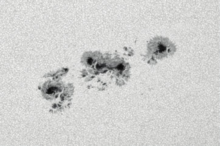
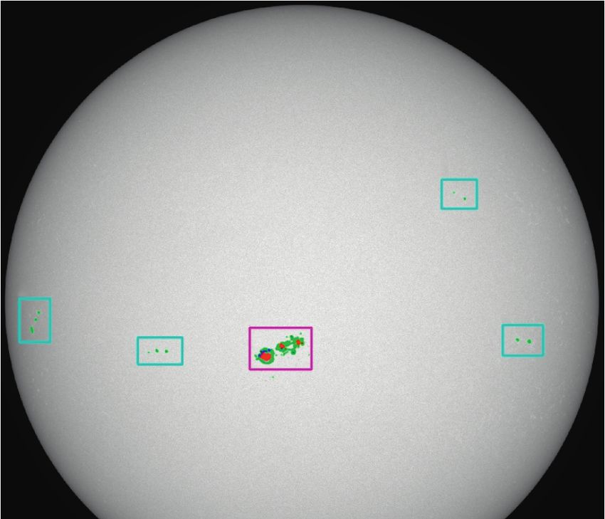
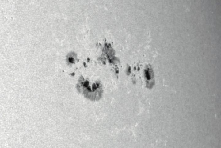
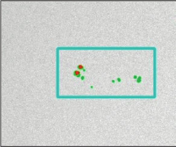
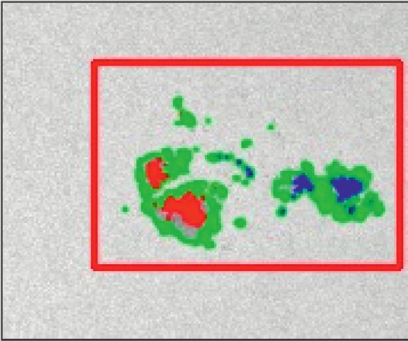
Advances in Astronomy 3

from the magnetogram into one image. The main steps are as numbers of samples differ greatly, which is due to the quite
follows (Figure 1): difference in occurrences of different types of sunspot
 groups. For example, the β type appears frequently, while the
 (1) The continuum image and the cotemporal magne-
 c type appears rarely. We had tried to solve the problem of
 togram are smoothed and normalized separately.
 the unbalanced numbers of the samples by oversampling.
 (2) The penumbra boundaries and umbra regions of the However, the experimental results show that the classifi-
 continuum image are extracted by the threshold cation effect is not significantly improved. Therefore, this
 method [22]. They are represented by A and B, re- paper does not do anything to balance the samples of various
 spectively. The positive and negative polar regions of types of sunspot groups.
 the magnetogram are extracted, which are repre-
 sented by C and D, respectively.
 (3) E � B ∩ C and F � B ∩ D, where E is the positive
 4. Method
 region of the umbra, and F is the negative region. ∩ We adopted a new deep learning model, CornerNet-Sac-
 is the intersection operation. cade, to implement the Mount Wilson magnetic classifi-
 (4) The penumbra boundaries corresponding to A in the cation of sunspot groups. It mainly includes three stages,
 continuum image are contoured with green; the generating object locations, detecting objects, and merging
 positive regions of the umbra corresponding to E are detections. The main flow of the method is shown in Fig-
 filled with red; and the negative regions of the umbra ure 2. The stage of generating object locations is plotted in
 corresponding to F are filled with blue. Figure 1 blue, which is to find approximate locations and rough sizes
 shows an example. Figure 1(a) is the continuum of the sunspot groups on the solar full images. The stage of
 image, Figure 1(b) is the magnetogram, and detecting objects is plotted in orange, which is to further
 Figure 1(c) is the composited image. determine the specific locations of the sunspot groups on the
 basis of the first stage and give the classification and con-
 A total of 2486 composited images were used to build the
 fidence score of the sunspot groups. The third stage of
Mount Wilson magnetic classification datasets. The training
 merging detections is plotted in red, which is to merge the
set is used to train the deep learning network model, which
 detections for eliminating the redundant boxes.
consists of 1886 composited images. The test set is used to
 The deep learning method needs training the network by
test the performance of the model, which consists of 600
 the samples in the training set first, which is to adjust the
composited images. The HMI data observed daily at 08:00:00
 parameters of networks by executing the feedforward
UT and 20:00:00 UT from 1 June 2010 to 31 December 2016
 propagation and back propagation in iterations. The
were mainly used for building the training set, and the data
 propagation algorithm performs a series of operations such
from 1 January 2017 to 30 April 2020 were used for the test
 as convolution and pooling to obtain the classification
set. All the samples were selected from them representa-
 probability and bounding box of the objects. The loss value
tively. The MDI data which were observed in July 2000
 of the loss function, which is used to evaluate the error
(NOAA 9601) and September 2001 (NOAA 9087) were
 between the estimated value and the true value, is then fed
supplements because there were no c and cδ types occurring
 back to the entire network by the back propagation algo-
from 2010 until April 2020 according to the Solar Region
 rithm; that is, the gradient of each layer of the networks is
Summary (SRS) text file (https://www.swpc.noaa.gov/). The
 calculated using the gradient descent algorithm to contin-
c and cδ types only appeared in NOAA 9601 and NOAA
 uously adjust the weight of each parameter to minimize the
9087 from 1996 until April 2020. Therefore, all the scarce
 loss. The training procedure is iterated until the loss value
data including c and cδ types were added to the training set
 converges steadily. The main steps, seen in Figure 2, are
and the test set without intersection. Besides that, some data
 detailed in the following (Figure 3).
including the βδ and βcδ types from 2010 to 2016 were
moved from the training set to the test set because these two (1) Downsizing the composited images for reducing
types have been relatively lacking since 2017. It should be inference time under limited memory.
noted that, from 1996 until now, the SRS file has not re- (2) Inputting the downsized images to the backbone
ported δ type. Therefore, the remainder of this paper no network, Hourglass-54 [37]. The Hourglass-54 net-
longer involves δ type. work is composed of three hourglass modules, which
 LabelMe tool [36] was used to label the samples of the has a total depth of 54 layers. Each hourglass is a
dataset. Each sample, a sunspot group, was given a label modular network with a symmetrical structure (see
according to the combination of the definition of Mount Figure 3). The hourglass network first applies three
Wilson magnetic classification [13] and the label of the SRS stages of convolution and downsampling layers to
file. If the label of a sunspot group from the SRS was reduce the size of the input feature maps and then
doubtful, then the label was mainly decided by the definition upsamples the features back to the original resolu-
of Mount Wilson magnetic classification. A total of 10,286 tion by three stages of convolution and upsampling
samples were labeled in the datasets, including 7805 samples layers, combining features across scales. Down-
in the training set and 2433 samples in the testing set. Table 1 sampling is achieved by convolution with stride of 2,
lists the numbers and proportions of all samples for various and upsampling is achieved by nearest neighbour
types of sunspot groups in the datasets. It can be seen that the interpolate [38]. One residual unit [39] is applied

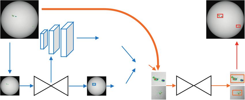
4 Advances in Astronomy

 2014.06.08

 (a) (b) (c)

Figure 1: An example of compositing the morphological structure information of sunspots from the continuum image and the magnetic
properties’ information from the magnetogram. The time is 20:00:00 UT on 8 June 2014. (a) The continuum image. (b) The magnetogram.
(c) The composited image, in which the penumbra boundaries of the sunspot groups are contoured with green, and the positive umbra
and the negative umbra are filled with red and blue, respectively.

Table 1: The numbers and proportions of the samples of various generates bounding boxes for the detected objects in
types. the downsized image. The bounding boxes are ob-
Type α β c cδ βc βδ βcδ tained by detecting the two key points, the top-left
 corners and the bottom-right corners of the object,
Number 2953 5086 13 28 1470 135 601
Proportion (%) 28.71 49.45 0.13 0.27 14.29 1.31 5.84 through corner pooling layers [33]. If the Intersec-
 tion over Union (IoU, Rezatofighi et al. [41]), the
 ratio of intersection and union of the bounding box
 after each downsampling layer and upsampling and ground truth, is greater than a threshold (set as
 layers, which corresponds to each box in Figure 3. 0.3 in this work), the bounding box is reserved
 Each residual unit is composed of two parts, three because it is more likely to contain the targets. So far,
 weight layers, and one identity mapping (or shortcut the approximate locations and sizes of the objects
 connections). Each weight layer is used to obtain from the attention maps and bounding boxes are
 deep-level information, which is designed as con- obtained separately.
 volutions and following ReLU (Conv-ReLU). The (4) the downsampled image at each possible location to
 identity mapping is used to retain the original in- find the locations of the objects more accurately. For
 formation, which is designed as a 1 × 1 convolution the locations obtained from the attention maps, the
 for matching dimensions with the output of the zoom ratios of small, medium, and large objects are
 weight layer. There are ten residual units in the commonly set as 4, 2, and 1, respectively. For the
 hourglass module, which better solves the vanishing locations obtained from the bounding boxes, the
 degradation problem of deep neural networks and downsized image is enlarged according to the size of
 improves the network performance. A total of three the bounding box.
 hourglass modules together allow for repeated bot- (5) the enlarged image back to the original image and
 tom-up, top-down inference across scales, which then cropping the regions by taking the locations as
 capture and consolidate information across all scales the center points.
 of the image. The outputs of Hourglass-54 are a set of
 feature maps. (6) the regions according to the scores and then picking
 up the top k locations with the highest scores.
 (3) Applying 3 × 3 Conv-ReLU module and a 1 × 1
 Conv-Sigmoid module on each feature map to (7) the possible objects in each region through the
 predict attention maps by the attention mechanism. second Hourglass-54. The bounding boxes of the
 The attention mechanism is derived from the sac- objects are fine adjusted by detecting the two key
 cades mechanism, which refers to a sequence of rapid points, the top-left corners and the bottom-right
 eye movements to fixate different image regions corners of the object, through the corner pooling
 [40].The feature maps at finer scales are used for layers.
 smaller objects and the ones at coarser scales are for (8) Training the network. The loss function of the model
 larger objects. A total of three size scales of attention consists of four losses with different weights [33]: a
 maps are predicted, corresponding to small, me- variant of focal loss, Ldet [42], the smooth L1 loss at
 dium, and large objects, respectively. The attention ground-truth corner locations, Loff [43], the loss of
 map indicates the approximate locations and rough grouping the corners, Lpull [44], and the loss of
 sizes of the object. Meanwhile, Hourglass-54 also separating the corners, Lpush [44].

Advances in Astronomy 5

 Attention maps

 Cropping regions
 Object locations
 (x0, y0)
 (x1, y1)

 Downsizing NMS
 (x2, y2)
 Attention (x0, y0)
 mechanism (x1, y1)

 Corner Ranking Corner
 (x2, y2) and picking
 pooling pooling
 Hourglass-54 Hourglass-54

Figure 2: The main flow of the network. The first stage of generating object locations is plotted in blue, which is to find approximate
locations and rough sizes of the sunspot groups on the solar full images. The second stage of detecting objects is plotted in orange, which is to
further determine the specific locations of the sunspot groups on the basis of the first stage and give the classification and confidence score of
the sunspot groups. The third stage of merging detection is plotted in red, which is to merge the detections for eliminating the redundant
boxes.

 Size

 Size/2

 Size/4

 Input Subsam. Subsam. Subsam. Upsam. Upsam. Upsam. Output
 Res. Res. Res.
 Res. Res.

 3 × 3, 384 3 × 3, 256 3 × 3, 256
 ReLU ReLU ReLU

 1 × 1, 256

Figure 3: An illustration of a single “hourglass” module. Each hourglass is a modular network with a symmetrical structure. Each box
represents a single residual module.

 (9) Testing the network. The feedforward propagation is maximum value and suppress nonlocal maximum
 performed only once with the flow of Figure 2, except values for each class, which aims to eliminate the
 for back propagation with loss functions. Besides redundant boxes of each class. This work modifies
 that, all detected bounding boxes are merged in the the typical NMS as eliminating the redundant boxes
 solar full image, where the redundant bounding for all bounding boxes as a whole, not repeating for
 boxes are eliminated based on Nonmaximum Sup- each class. On average, it takes about three seconds to
 pression (NMS) [45]. The typical NMS is to find local process one image.

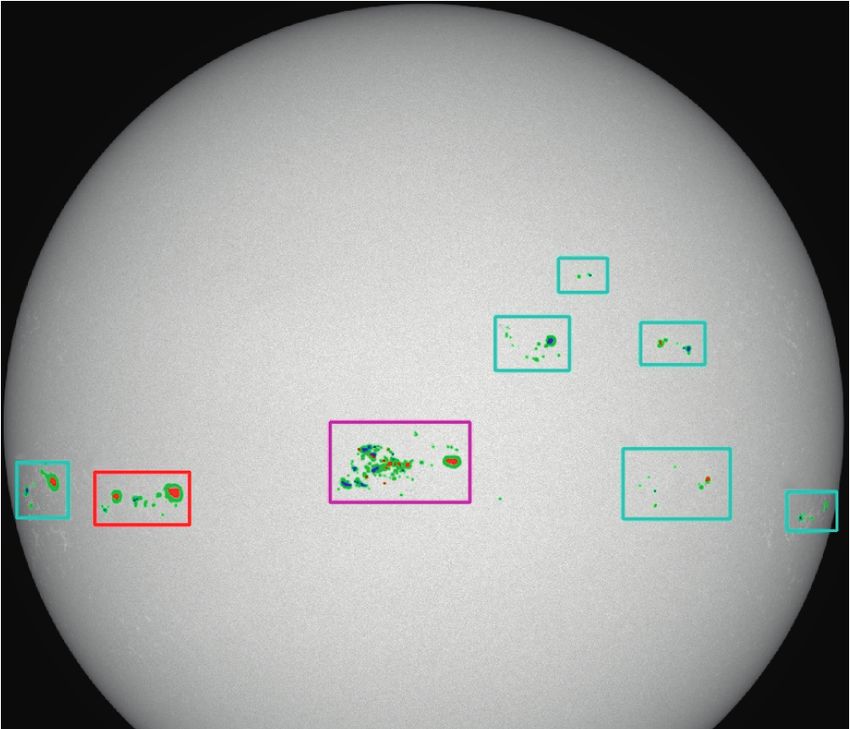
6 Advances in Astronomy

 The experiments were performed on a personal computer where N is the total number of samples. The true positive,
equipped with a GeForce RTXTM 2080 graphics card. The TP, is the number of items correctly labeled as belonging to
main programs deployed were Python 3.7, PyTorch 1.2, the positive class. The false positive, FP, is the number of
CUDA 10.1, GCC 7.4, etc. Adam [46] was chosen to optimize items incorrectly labeled as belonging to the class. The false
both losses for the attention maps and object detections. After negative, FN, is the number of items which are not labeled as
repeated experiments, the hyperparameters such as the belonging to the positive class but should have been. The
learning_rate, decay_rate, batch_size, and IoU of the network average precision, AP, is a typical performance metric of
model were set to 0.000025, 10, 8, and 0.01, respectively. The combination of precision and recall, which is calculated as
loss value of the network converges stably after 335,000 it- the precision averaged across all recall values between 0 and
erations of training, which takes about 110 hours. 1.
 Table 2 lists the metrics of the test set. Note that c and cδ
 are not taken into account in Table 2, because there are few c
5. Results and cδ types of sunspot groups in the training set and the test
5.1. Instance. Figure 4 shows two cases. The sunspot groups set. It is meaningless to evaluate their corresponding per-
with solid line boxes are detected by our method, where the formances. The mean accuracy, precision, recall, and mean
classification results are displayed at the upper left of each AP (mAP) are all above 0.90. There are three types in which
box. The active region (AR) number and classification of the the AP values reach up to 0.90, namely, β, βc, and βcδ. On
sunspot groups given by NOAA are manually labeled to the the other hand, the APs of α and βδ types are a little lower
box below. Note that the reports of NOAA are issued on than 0.90. We found that some small sunspots belonging to α
today using data from yesterday. We marked them by using type are easily confused with the background, which results
the correct reports. in false detections and missed detections. The βδ type has
 It can be seen in Figure 4(a) that our method detects five some characteristics confused with β, βc, and βcδ, so there
sunspot groups. A total of three sunspot groups are marked are a few false detections.
by NOAA: NOAA 12299, NOAA 12297, and NOAA 12298.
Our classification results are consistent with them, where the
 5.3. Statistics. Based on the satisfactory results of this
three sunspot groups are classified into β, βcδ, and β, re-
 method, the solar full images of HMI from January 2011 to
spectively. Besides that, two other sunspot groups (red ar-
 April 2020 were fed to the trained network for the Mount
rows 1 and 2) are detected by our method, and both of them
 Wilson magnetic classification of sunspot groups. A total of
are classified into β type.
 3086 composited images are available; most of them are at
 In Figure 4(b), eight sunspot groups are detected by our 20:00:00 UT and a few of them are near 20:00:00 UT. As a
method, while seven are marked by NOAA. There are six result, a total of 11, 681 sunspot groups are detected and
sunspot groups that are the same by NOAA and by our classified. Note that only five types of sunspot groups
method. NOAA 11971 (red arrow 3) is classified as β type by appeared in this decade. They are α, β, βc, βδ, and βcδ, where
our method; however, it is classified as α type by NOAA. By the numbers are 3951, 6094, 1158, 110, and 368, respectively.
analyzing the continuum image and the corresponding Therefore, only these five types are analyzed in this section.
magnetogram, this sunspot group is a bipolar group, where Detailed data are shared on the website (https://61.166.157.
there is no mixed polarity and no umbra of opposite polarity 71/MWMCSG.html).
in the same penumbra region. Therefore, the sunspot group We summarized the total number for each type of
ought to be β type. Besides that, there is a visible sunspot sunspot group in months in Figure 5. The x-axis represents
group above NOAA 11973 (red arrow 4). Our method detects time in months, and the y-axis represents the number of
the sunspot group and classifies it into β type correctly. sunspot groups. Because no data are provided in some days,
 we fill the missed data by averaging the previous day and the
 next day in order to plot the lines continuously in the figure.
5.2. Evaluation Metrics. We evaluated the performance of The number of sunspot groups belonging to the same
our method by four metrics: accuracy, precision, recall, and type varies greatly over time. For α type, the highest
AP [47]. The definitions are as follows: number is 106 in December 2014; the lowest number falls to
 1 in February 2020. The difference between the maximum
 TP value and minimum value reaches up to 105. For β type,
 accuracy � ,
 N there are two months with the highest number of 144,
 including November 2011 and May 2013. On the other
 TP hand, the lowest number is 0 in October 2019. Besides that,
 precision � ,
 TP + FP the other types are relatively rare. The highest numbers of
 (1) βc and βδ are 49 and 12, respectively, which occur in
 TP
 recall � , February 2014 and November 2014, respectively. For βcδ
 TP + FN type, there are two months with the highest number of 18:
 1 July 2012 and October 2013. For βc, βδ, and βcδ, there are
 AP � P(r)dr, 24, 63, and 54 months with the lowest numbers of 0,
 0
 respectively.

Advances in Astronomy 7

 4
 β β

 β β
 2

 NOAA 11973: β NOAA 11978: β
 β βγδ
 β
 βγδ β β
 β βγ
 β
 NOAA 12299: β
 NOAA 12298: β NOAA 11974: βγδ
 NOAA 12297: βγδ NOAA 11977: β NOAA 11971: α
 1 NOAA 11976: βγ NOAA 11975: β
 3

 2015.03.12 2014.02.11

 (a) (b)

Figure 4: Two cases. The sunspot groups with solid-line boxes are detected by our method, where the classification results are displayed at
the upper left of each box. The AR number and classification given by NOAA are manually labeled at the box below. The times of (a) and (b)
are 20:00:00 UT on 12 March 2015 and 20:00:00 UT on 11 February 2014, respectively.

 Table 2: The metrics of the test set.
Type Accuracy Recall Precision AP
α 0.90 0.92 0.90 0.89
β 0.95 0.94 0.95 0.93
βc 0.94 0.92 0.94 0.90
βδ 0.93 0.91 0.93 0.87
βcδ 0.96 0.95 0.96 0.93
Mean 0.94 0.93 0.94 0.90

 Solar activity level is closely related to three types of 5.4. The Relationship between Magnetic Classification and
sunspot groups, such as α, β, and βc. From 2011 to 2016, Solar Flares. Solar flares are closely related to the magnetic
there are a great number of α, β, and βc types. In particular, α classification of sunspot groups. The solar flare productivity
and β types have hundreds of numbers monthly, where the is used to quantify the relationship, which is calculated by
sun is relatively active during this period. Since 2016, these the total number of flares divided by the number of sunspot
types of sunspot groups have gradually decreased, even groups. According to the peak fluxes of soft X-ray, flares are
down to single digits, where the solar activities decrease. On usually classified into four levels: B, C, M, and X. Within a
the contrary, the numbers of βδ and βcδ types have a little certain time interval, the total importance, Itot , is presented
change, where the monthly amounts are only 12 and 18 at as [48, 49]
the peak, respectively.
 The numbers of various types differ significantly in the Itot � 0.1 × B + 1.0 × C + 10 × M + 100 × X.
same period of time, especially during the solar active pe- (2)
riod. For example, in November 2011 (the left-dashed
vertical line), the numbers of α, β, βc, βδ, and βcδ are 76, The flare productivity with Itot ≥ 1, which is equivalent
144, 29, 5, and 7, respectively. The maximum difference to a C1.0 flare, is analyzed. The occurrence of flares in an AR
(between β and βδ) is up to 139. But, with the solar activity described in this paper is within 48 hours. The solar flare data
weakening, the difference becomes smaller. For example, in come from the NOAA website (https://www.solarmonitor.
February 2020 (the right vertical line), the number of α, β, org/). The number of sunspot groups and the corresponding
βc, βδ, and βcδ are 1, 1, 0, 0, and 0, respectively. The flare productivity from January 2011 to April 2020 are listed
maximum difference (between β and βδ) is only 1. in Table 3. They are also plotted in Figure 6 in order to make

8 Advances in Astronomy

 200
 190
 180
 170
 160
 150
 140
 130
 120
 110
 Number

 100
 90
 80
 70
 60
 50
 40
 30
 20
 10
 0
 2011 2012 2013 2014 2015 2016 2017 2018 2019 2020 2021
 Month
 α βδ
 β βγδ
 βγ
Figure 5: The total number for each type of sunspot groups in months from January 2011 to April 2020. The left dashed vertical line
(November 2011) represents that the numbers of various types differ significantly, where the maximum difference is up to 139. The right
dashed vertical line (February 2020) represents the numbers of various types that are very close, where the maximum difference is only 1.

 Table 3: The number of various types of the sunspot groups and the corresponding flare productivity from 2011 to 2020 (Itot ≥ 1).
 Numbers of Numbers of C- Numbers of M- Numbers of X- Productivity of C- Productivity of M- Productivity of X-
Type
 sunspot groups class flares class flares class flares class flares class flares class flares
α 649 91 15 0 0.14 0.02 0
β 1044 297 71 5 0.28 0.07 0.01
βc 336 206 91 7 0.61 0.27 0.02
βδ 49 35 22 5 0.71 0.45 0.10
βcδ 105 91 68 23 0.87 0.65 0.22
Total 2183 720 267 40 0.33 0.12 0.02

 1

 0.8

 0.6

 0.4

 0.2

 0
 α β βγ βδ βγδ
 C-class
 M-class
 X-class
Figure 6: Productivity of C-class, M-class, and X-class flares of various types of the sunspot groups from January 2011 to April 2020
(Itot ≥ 1).

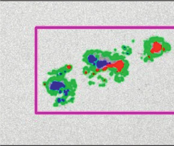
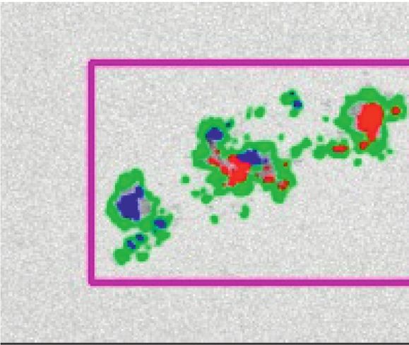
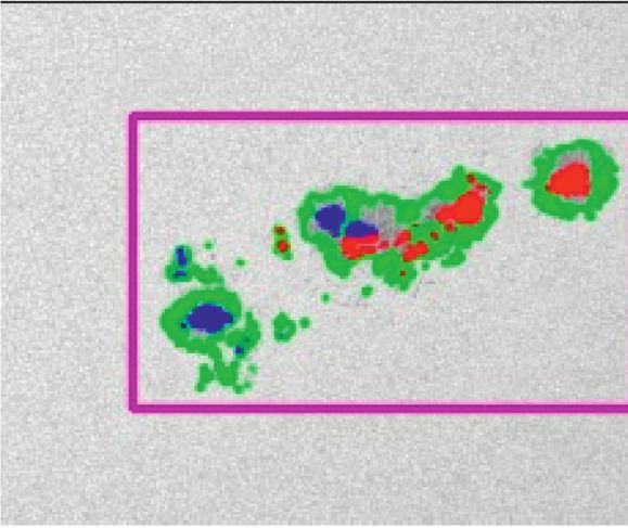
Advances in Astronomy 9

the relationship between magnetic classification of sunspot in this year are very abundant. There are a few sunspots in
groups and flare productivities more intuitive. some days and very big sunspots in other days. Importantly,
 It is found that the more complex the sunspot group is, a lot of different levels of flares erupted in that year.
the higher the corresponding flare productivity is. For in- Therefore, it is a typical year that we chose for analyzing the
stance, the flare productivities of C, M, and X belonging to magnetic classification of sunspot groups day by day. The x-
the α type are all lower than those belonging to the β types axis represents the classification of sunspot groups, and the
(including β and βc types), and those of the β types are all y-axis represents the number of each type. Our results are
lower than those of the δ types (including βδ and βcδ types). very similar to those of NOAA. The total numbers detected
In detail, the flare productivities of C-class, M-class, and by our method and NOAA are 2254 and 2073, respectively.
X-class belonging to α are 0.14, 0.02, and 0, respectively; and In detail, there are 654 sunspot groups belonging to α type by
those belonging to β are 0.28, 0.07, and 0.01, respectively. our method, 57 more than NOAA; 1155 β sunspot groups,
The flare productivities of these two types of sunspot groups 129 more than NOAA; 302 βc sunspot groups, 8 less than
are relatively low; in particular, X-class is almost zero. It NOAA; 23 βδ sunspot groups, 4 more than NOAA; and 120
means that these two types of sunspot groups with simple βcδ sunspot groups, 1 less than NOAA. The main reason
structures are difficult to produce large flares. On the other why there are more α and β types by our method than those
hand, the flare productivities of βc, βδ, and βcδ are relatively by NOAA is that our method detects more of small α and β
high. The values for C-class flares reach up to 0.61, 0.71, and sunspot groups. On the other hand, the sum of the βc, βδ,
0.87, respectively, and those for M-class flares are 0.27, 0.45, and βcδ sunspot groups detected by our method is 445, and
and 0.65, respectively. The X-class flares are very rare, as only that by NOAA is 450. The total difference is very small, and
forty occurred in the last ten years. The corresponding flare the difference of every type is also very small. We found that
productivities of βc, βδ, and βcδ are 0.02, 0.10, and 0.22, the difference is mainly caused by the somewhat similar
respectively. Especially, for a total of 105 βcδ, there erupted features of these types during the evolution of sunspot
23 X-class flares. That means βc, βδ, and βcδ have much groups (see Figure 7). Note that the statistical results are
higher probabilities of flare eruption than the other types, obtained by 313 days in 2014 due to missed data.
especially βcδ. In additional, X-class flares basically occur Figure 10 shows the flare productivities by our method
above the δ or c types. and NOAA in 2014. Here, the total flare level, Itot , is set to 10
 The above results show that the Mount Wilson magnetic or greater, which is equivalent to an M1.0 flare. The flares
classification of sunspot groups is indeed closely related to productivities of α, β, βc, βδ, and βcδ detected by our method
solar flares. Therefore, the magnetic classification can be are 0.03, 0.10, 0.37, 0.60, and 0.64, respectively. They are 0.05,
used as a major factor to predict the flare eruptions. 0.15, 0.37, 0.40, and 0.48 by NOAA, respectively. The general
 trends of the flare productivities of different types by our
6. Discussion method and NOAA are similar. The more complex the
 sunspot group is, the higher its flare productivity is. In other
6.1. Comparison with NOAA. We compared our results with words, the flare productivities of βcδ, βδ, and βc are both
NOAA carefully. Figure 7 shows the evolving procedure and higher than that of β, and that of β is higher than that of α. If
classification results of NOAA 11158 from 13 to 15 February we have to say something different, NOAA obtains higher
2011. flare productivities of α and β compared to our method; our
 It can be seen that the sunspot group during the three method has the same flare productivity as NOAA for βc; for
days is mixed in polarity, with opposite polarity within the βδ and βcδ that are most closely related to flares, the flare
same penumbra and no more than 2∘ separation of the productivities of our method are higher than those of NOAA.
umbra in the continuum image and the corresponding Note that the numbers of sunspot groups are counted
magnetogram. According to the description of Mount somewhat differently in Figures 9 and 10. The number of
Wilson magnetic classification, the sunspot group should be sunspot groups in Figure 9 is the number of occurrences of
βcδ. The results obtained by our method are all βcδ, while sunspot groups in days, but in Figure 10, it is the number of
NOAA gives βc on the 13th and the 14th and βcδ on the different types of sunspot groups in their evolutions. For
15th. X-class large flares erupted above NOAA 11158 on the example, NOAA 11946 appeared on 5 January 2014 and
14th. Our method classifies it into βcδ two days earlier than disappeared on the 12th. It belongs to β in three days and to
NOAA and one day earlier than the eruption of this large βc in five days. The numbers of β and βc in Figure 9 are 3 and
flare. 5, respectively, while both are 1 in Figure 10.
 Figure 8 shows the evolving procedure and classification In summary, the multilevel features of various types of
results of NOAA 12260 from 8 to 10 January 2015. There is sunspot groups are extracted effectively using the deep
an AR visible at the lower right corner of NOAA 12258 on 8 learning method. This leads to a good performance in the
January 2015. Our method detects the AR and classifies it magnetic classification of sunspot groups. Moreover, the
into β in time. This AR is marked as NOAA 12260 and complex sunspot groups including βc, βδ, and βcδ have
classified into β by NOAA on the 9th. Our method detects higher flare productivities, especially βcδ. Most X-class solar
the AR one day earlier than NOAA. flares erupt above the complex sunspot groups. The Mount
 Moreover, we counted the numbers of various types of Wilson magnetic classification of the sunspot groups can
sunspot groups detected by our method and NOAA in 2014 indeed be used as an important predictor to predict the
separately, as shown in Figure 9. The types of sunspot groups eruption of solar flares.

10 Advances in Astronomy

 βγδ

 NOAA 11158: βγ
 2011.02.13
 (a) (b) (c)

 βγδ

 NOAA 11158: βγ
 2011.02.14
 (d) (e) (f )

 βγδ

 NOAA 11158: βγδ
 2011.02.15
 (g) (h) (i)

Figure 7: The classifications of NOAA 11158 given by our method and NOAA. The columns from left to right are the continuum image,
magnetogram, and the classification result. The rows are the evolving procedure, which is on the 13th, 14th, and 15th of February 2011,
respectively. All the times are 20:00:00 UT. The sunspot groups with solid-line boxes are detected by our method, where the classification
results are displayed at the upper left of each box. The AR number and classification given by NOAA are manually labeled at the box below.

6.2. Some Problems. Although our method has achieved a 2012, respectively. In Figure 12(a), the sunspot group is
good performance in the Mount Wilson magnetic classifi- about to disappear from the solar surface. On the other hand,
cation of sunspot groups, there are still some problems. the sunspot group in Figure 12(b) just appears on the solar
 Some small spots are difficult to be affirmed because they surface. Both of them are classified into α type by our
are very similar to background. Figure 11(a) shows the result method. However, the characteristics of these sunspot
by our method on 2 August 2011. A total of four sunspot groups are not fully shown. It is difficult to judge whether it
groups are detected and classified. Two regions with red is true. For such situations, it is not easy to classify them
circle labeled as 1 and 2 are zoomed in panels 11(b) and accurately even by hand.
11(c). Neither our method nor NOAA detects Region 1 as an Moreover, some sunspot groups are difficult to be
AR, but both of them detect Region 2 as an AR (NOAA classified during their evolution according to the definition
11264). The difference is that our method classifies Region 2 of the Mount Wilson magnetic classification of sunspot
into α, while NOAA does not give a classification result. It is groups. Figure 13 shows one common example, NOAA
not difficult to see that these two small spots are very similar. 12257, from 9 to 11 January 2015. The sunspot group is
The main reason for miss-detected Region 1 is its envi- judged as βc by our method but as βδ by NOAA on 9 January
ronment. The reason is possibly due to the downsized images 2015. We think that it should not be δ because of the umbra
in order to reduce memory consumption. We believe this with the same polarity in the same penumbra. However,
problem can be solved if the hardware conditions can whether it belongs to β or βc is not easy to distinguish
support the high-resolution image without downsizing for clearly. The main reason is that there are some unclear words
deep learning operations. in the definition, such as simple, complex, and irregular. For
 Some sunspot groups are difficult to be judged when they instance, β is a bipolar sunspot group, with the simple and
are located at the edge of the solar surface. Figures 12(a) and obvious division between polarities; c is a complex sunspot
12(b) are subregions observed on May 10 2012 and 6 August group with irregular polarity; βc is a bipolar sunspot group

Advances in Astronomy 11

 β

 2015.01.08
 (a) (b) (c)

 β

 NOAA 12260: β

 2015.01.09
 (d) (e) (f )

 β

 NOAA 12260: β

 2015.01.10
 (g) (h) (i)

Figure 8: The classifications of NOAA 12660 given by our method and NOAA. The columns from left to right are the continuum image,
magnetogram, and the classification result. The rows are the evolving procedure, which is on the 8th, 9th, and 10th of January 2015,
respectively. All the times are 20:00:00 UT. The active region appeared on 8 January 2015. Our method detects the active region and classifies
it into β in time. This AR is marked as NOAA 12260 and is classified into β on the 9th by NOAA.

 2500

 2000

 1500

 1000

 500

 0
 α β βγ βδ βγδ Sum
 NOAA
 Our method
 Figure 9: The numbers of various types of sunspot groups detected by our method and NOAA in 2014.

but with more than one continuous polarity reversal line. Here, it is judged by our method to be βc. Now, in the second
What level is simple or complex especially in the transitional row that follows, it is judged as δ because of the umbra with
period from one type into another type during its evolution? opposite polarity appear in the same penumbra, which are

12 Advances in Astronomy

 0.7

 0.6

 0.5

 0.4

 0.3

 0.2

 0.1

 0
 α β βγ βδ βγδ
 NOAA
 Our method
 Figure 10: The flare productivities of various types of sunspot groups detected by our method and NOAA in 2014 (Itot ≥ 10).

 α

 2
 1

 β
 βγδ βγδ
 1
 NOAA 11264

 α
 2

 2011.08.02

 (a) (b) (c)

Figure 11: Detection results by our method at 20:00:00 UT on 2 August 2011. (a) The detection results of the composited solar full image.
The region with a red circle labeled as 1 is not detected, which is zoomed in (b). The region labeled as 2 is detected, which is zoomed in (c).

 α α

 2012.05.10 2012.08.06

 (a) (b)

Figure 12: (a, b) Subregions at the edges of the solar surface observed at 20:00:00 UT on 10 May 2012 and at 20:00:00 UT on 6 August 2012,
respectively.

Advances in Astronomy 13

 βγ

 NOAA 12257: βδ
 2015.01.09
 (a) (b) (c)

 βγδ

 NOAA 12257: βδ
 2015.01.10
 (d) (e) (f )

 βγδ

 NOAA 12257: βγδ
 2015.01.11
 (g) (h) (i)

Figure 13: The classifications of NOAA 12257 given by our method and NOAA. The columns from left to right are the continuum image,
magnetogram, and the detection result, respectively. The rows show the evolving procedure, which is on the 9th, 10th, and 11th of January
2015, respectively. All the times are 20:00:00 UT. The sunspot groups with solid-line boxes are detected by our method, where the
classification results are displayed at the upper left of each box. The AR numbers and classification given by NOAA are manually labeled at
the box below.

coincident by both methods. Whether it belongs to β or βc is classification, which are divided into a training set and a test
also a problem. We think that the sunspot group is inclined set at a ratio of 3 : 1.
to be βcδ for its complex sunspot group with irregular A deep learning model, CornerNet-Saccade, is adopted
polarity here. In the third row, both methods obtain the to detect and classify the sunspot groups. It mainly includes
same results, βcδ. three stages, generating object locations, detecting objects,
 and merging detections. The first stage is to find approximate
7. Conclusion locations and rough sizes of the sunspot groups on the solar
 full images. The backbone of the method is Hourglass-54,
This paper proposes a deep learning method for the Mount which consists of 3 hourglass modules with a total depth of
Wilson magnetic classification of sunspot groups. The 54 layers. Each hourglass module is a symmetrical structure,
continuum images and the magnetograms from HMI which downsamples to a very low resolution and then
spanning from June 2010 to April 2020 and MDI spanning upsamples and combines features across multiple resolu-
from July 2000 to September 2001 are employed to build the tions. The multiple hourglass modules together allow for
dataset. We first composite the morphological structures of repeated bottom-up, top-down inference across scales,
sunspot groups from the continuum image and the magnetic which capture and consolidate information across all scales
properties from the cotemporal magnetogram into one of the image. A total of three size scales of attention maps are
image. A total of 2486 composited images are then labeled to predicted using the feature maps gotten from Hourglass-54
build the dataset of the Mount Wilson magnetic by the attention mechanism, corresponding to small,

14 Advances in Astronomy

medium, and large objects. Meanwhile, the bounding boxes downloaded from https://jsoc.stanford.edu/. The SRS text
are generated by detecting the two key points, the top-left files can be downloaded from the NOAA/SWPC website
corners and the bottom-right corners of the object, through https://www.swpc.noaa.gov/. The training set and test set
corner pooling layers. The second stage is to further de- data for deep learning of this study are available from the
termine the specific locations and bounding boxes of the corresponding author upon request.
sunspot groups. The locations gotten from the first stage are
ranked by their scores, and then the top ones are picked up.
They are fine-adjusted by corner pooling layers using the
 Conflicts of Interest
feature maps through the second Hourglass-54. The third The authors declare that there are no conflicts of interest
stage is to merge the detections by NMS for eliminating the regarding the publication of this paper.
redundant boxes. These key technologies improve the effi-
ciency of the deep learning method without sacrificing
accuracy. Acknowledgments
 The model is trained on a personal computer equipped
 The authors are grateful for the support received from the
with a GeForce RTXTM 2080 graphics card. After 335,000
 National Natural Science Foundation of China (nos. 11763004,
iterations, the loss value converges stably. It takes about 3
 11573012, 11803085, 12063003, and U1931107) and the Open
seconds to detect and classify the sunspot groups in a
 Research Program of the Key Laboratory of Solar Activity of
composited solar full image. The experimental results show
 the Chinese Academy of Sciences (no. KLSA202019). This
that this method has an excellent performance in the de-
 work was also supported by the National Key Research and
tection and classification. The accuracy, precision, recall, and
 Development Program of China (2018YFA0404603), Yunnan
mAP reach up to 0.94, 0.93, 0.94, and 0.90, respectively.
 Key Research and Development Program (2018IA054), and
 Based on the reliable performance of our method, the
 Yunnan Applied Basic Research Project (2018FB103). The
classifications of sunspot groups in the past 10 years from
 continuum images and magnetograms used in this study were
January 2011 to April 2020 are analyzed, which are shared on
 kindly provided by SDO and SOHO. The text files were kindly
the website (https://61.166.157.71/MWMCSG.html). In ad-
 provided by NOAA/SWPC. The authors thank them for
dition, we calculate the flare productivities of various types
 maintaining and providing the data.
of sunspot groups from January 2011 to April 2020 in order
to describe the relationship between the magnetic classifi-
cation of sunspot groups and solar flares. If Itot is set to References
greater than or equal to 1, the flare productivities of α, β, βc,
βδ, and βcδ sunspot groups are 0.14, 0.28, 0.61, 0.71, and [1] K. Sakurai, “Motion of sunspot magnetic fields and its relation
0.87, respectively. If Itot is set to greater than or equal to 10, to solar flares,” Solar Physics, vol. 47, no. 1, pp. 261–266, 1976.
 [2] P. O. Taylor, “The relationship between sunspot and solar flare
they are 0.02, 0.07, 0.27, 0.45, and 0.65, respectively. Among
 activities for the period 1974–1987,” Journal of the American
them, the flare productivities of βc, βδ, and βcδ reach up to Association of Variable Star Observers, vol. 17, pp. 20-21, 1988.
0.60 with Itot ≥ 1. The productivities of βδ and βcδ reach up [3] Z. Shi and J. Wang, “Delta-sunspots and X-class flares,” Solar
to 0.45 even with Itot ≥ 10. This means that βc, βδ, and βcδ Physics, vol. 149, no. 1, pp. 105–118, 1994.
sunspot groups are indeed very closely related to solar flare [4] M. Hahn, S. Gaard, P. Jibben, R. C. Canfield, and D. Nandy,
eruptions, especially the βcδ sunspot groups. “Spatial relationship between twist in active region magnetic
 We also compare the classifications of sunspot groups fields and solar flares,” The Astrophysical Journal, vol. 629,
with NOAA using the data in 2014. The results show that our no. 2, pp. 1135–1140, 2005.
method detects more α and β sunspot groups which are [5] Y. Cui, R. Li, H. Wang, and H. He, “Correlation between solar
small and faint; therefore, the numbers of α and β are 654 flare productivity and photospheric magnetic field properties
 II. Magnetic gradient and magnetic shear,” Solar Physics,
and 1155, respectively, 57 and 129 more than those of
 vol. 242, no. 1-2, pp. 1–8, 2007.
NOAA, respectively. Our method is good at distinguishing [6] Y. Zhang, J. Liu, and H. Zhang, “Relationship between ro-
the more complex sunspot groups including βc, βδ, and βcδ tating sunspots and flares,” Solar Physics, vol. 247, no. 1,
classes, owing to the features of different types learned by the pp. 39–52, 2008.
deep learning networks, where the detection schemes of [7] A. G. Emslie, B. R. Dennis, A. Y. Shih et al., “Global energetics
CornerNet-Saccade, such as Hourglass-54, key points, and of thirty-eight large solar eruptive events,” The Astrophysical
the attention map mechanism, make the features of the Journal, vol. 759, no. 1, p. 71, 2012.
multiple levels fused available. [8] M. Zhao, J. Chen, and Y. Liu, “Statistical analysis of sunspot
 In the future, we plan to use the Mount Wilson magnetic groups and flares for solar maximum and minimum,” Scientia
classification of sunspot groups as the main predictor to Sinica Physica, Mechanica & Astronomica, vol. 44, pp. 109–
establish a more reasonable solar flare prediction model. 120, 2014.
 [9] K. O. Kiepenheuer, “Solar activity,” in The Sun, p. 322, 1953.
 [10] A. L. Cortie, “On the types of sun-spot disturbances,” The
Data Availability Astrophysical Journal, vol. 13, p. 260, 1901.
 [11] P. Simon, G. Heckman, and M. Shea, COSPAR: Solar-ter-
The magnetogram and continuum image data used to restrial Predictions: Proceedings of a Workshop at Meudon,
support the findings of this study are observed by SDO/HMI France, June 18-22, 1984, National Oceanic and Atmospheric
and SOHO/MDI; all of the FITS files we have used are Administration, Washington, DC, USA, 1986.

Advances in Astronomy 15

[12] P. S. McIntosh, “The classification of sunspot groups,” Solar [32] X. Wang, K. Chen, Z. Huang, C. Yao, and W. Liu, “Point
 Physics, vol. 125, no. 2, pp. 251–267, 1990. linking network for object detection,” 2017, https://arxiv.org/
[13] G. E. Hale, F. Ellerman, S. B. Nicholson, and A. H. Joy, “The abs/1706.03646.
 magnetic polarity of sun-spots,” The Astrophysical Journal, [33] H. Law and J. Deng, “CornerNet: detecting objects as paired
 vol. 49, p. 153, 1919. keypoints,” 2018, https://arxiv.org/abs/1808.01244.
[14] X. L. Yan, L. H. Deng, Z. Q. Qu, and C. L. Xu, “The phase [34] P. H. Scherrer, J. Schou, R. I. Bush et al., “The helioseismic and
 relation between sunspot numbers and soft X-ray flares,” magnetic imager (HMI) investigation for the solar dynamics
 Astrophysics and Space Science, vol. 333, no. 1, pp. 11–16, 2011. observatory (SDO),” Solar Physics, vol. 275, no. 1-2,
[15] G. R. Greatrix, “On the statistical relations between flare pp. 207–227, 2012.
 intensity and sunspots,” Monthly Notices of the Royal As- [35] P. H. Scherrer, R. S. Bogart, R. I. Bush et al., “The solar os-
 tronomical Society, vol. 126, no. 2, pp. 123–133, 1963. cillations investigation-Michelson Doppler imager,” Solar
[16] I. Sammis, F. Tang, and H. Zirin, “The dependence of large Physics, vol. 162, no. 1-2, pp. 129–188, 1995.
 flare occurrence on the magnetic structure of sunspots,” The [36] B. C. Russell, A. Torralba, K. P. Murphy, and W. T. Freeman,
 Astrophysical Journal, vol. 540, no. 1, pp. 583–587, 2000. “LabelMe: a database and web-based tool for image anno-
[17] S. Eren, A. Kilcik, T. Atay et al., “Flare-production potential tation,” International Journal of Computer Vision, vol. 77,
 associated with different sunspot groups,” Monthly Notices of no. 1–3, pp. 157–173, 2008.
 the Royal Astronomical Society, vol. 465, no. 1, pp. 68–75, [37] A. Newell, K. Yang, and J. Deng, “Stacked hourglass networks
 for human pose estimation,” 2016, https://arxiv.org/abs/1603.
 2017.
 06937.
[18] T. T. Nguyen, C. P. Willis, D. J. Paddon, S. H. Nguyen, and
 [38] O. Rukundo and H. Cao, “Nearest neighbor value interpo-
 H. S. Nguyen, “Learning sunspot classification,” Fundamenta
 lation,” 2012.
 Informaticae, vol. 72, pp. 295–309, 2006.
 [39] K. He, X. Zhang, S. Ren, and J. Sun, “Deep residual learning
[19] M. A. Abd, S. F. Majed, and V. Zharkova, “Automated
 for image recognition,” 2015, https://arxiv.org/abs/1512.
 classification of sunspot groups with support vector ma-
 03385.
 chines,” in Technological Developments in Networking, Edu- [40] B. W. Tatler, N. J. Wade, H. Kwan, J. M. Findlay, and
 cation and Automation, K. Elleithy, T. Sobh, M. Iskander, B. M. Velichkovsky, “Yarbus, eye movements, and vision,” I-
 V. Kapila, M. A. Karim, and A. Mahmood, Eds., Springer, Perception, vol. 1, no. 1, pp. 7–27, 2010.
 Dordrecht, Netherlands, 2010. [41] H. Rezatofighi, N. Tsoi, J. Gwak, A. Sadeghian, I. Reid, and
[20] T. Colak and R. Qahwaji, “Automated Solar Activity Pre- S. Savarese, “generalized intersection over union: a metric and
 diction: a hybrid computer platform using machine learning a loss for bounding box regression,” 2019, https://arxiv.org/
 and solar imaging for automated prediction of solar flares,” abs/1902.09630.
 Space Weather, vol. 7, no. 6, 2009. [42] T. Y. Lin, P. Goyal, R. Girshick, K. He, and P. Dollár, “Focal
[21] S. Hong, J. Kim, J. Han, and Y. Kim, “The automatic solar loss for dense object detection,” 2017, https://arxiv.org/abs/
 synoptic analyzer and solar wind prediction,” AGU Fall 1708.02002.
 Meeting Abstracts, vol. 2014, pp. SH21A–4089, 2014. [43] R. Girshick, “Fast R-CNN,” 2015, https://arxiv.org/abs/1504.
[22] S. Padinhatteeri, P. A. Higgins, D. Shaun Bloomfield, and 08083.
 P. T. Gallagher, “Automatic detection of magnetic δ in [44] A. Newell and J. Deng, “Pixels to graphs by associative em-
 sunspot groups,” Solar Physics, vol. 291, no. 1, pp. 41–53, 2016. bedding,” 2017, https://arxiv.org/abs/1706.07365.
[23] Y. Fang, Y. Cui, and X. Ao, “Deep learning for automatic [45] A. Neubeck and L. Gool, “Efficient non-maximum suppres-
 recognition of magnetic type in sunspot groups,” Advances in sion,” in Proceedings of the 18th International Conference on
 Astronomy, vol. 2019, pp. 1–10, 2019. Pattern Recognition (ICPR’06), pp. 850–855, Hong Kong,
[24] Y. LeCun, L. Bottou, Y. Bengio, and P. Haffner, “Gradient- August 2006.
 based learning applied to document recognition,” Proceedings [46] D. P. Kingma and J. Ba, “Adam: a method for stochastic
 of the IEEE, vol. 86, no. 11, pp. 2278–2324, 1998. optimization,” 2014, https://arxiv.org/abs/1412.6980.
[25] G. E. Hinton and R. R. Salakhutdinov, “Reducing the di- [47] M. Everingham, L. Van Gool, C. K. I. Williams, J. Winn, and
 mensionality of data with neural networks,” Science, vol. 313, A. Zisserman, “The pascal visual object classes (VOC) chal-
 no. 5786, pp. 504–507, 2006. lenge,” International Journal of Computer Vision, vol. 88,
[26] Y. LeCun, Y. Bengio, and G. Hinton, “Deep learning,” Nature, no. 2, pp. 303–338, 2010.
 vol. 521, no. 7553, pp. 436–444, 2015. [48] A. Antalova, “Daily soft X-ray flare index (1969–1972),”
[27] R. Girshick, J. Donahue, T. Darrell, and J. Malik, “Rich feature Contributions of the Astronomical Observatory Skalnate Pleso,
 hierarchies for accurate object detection and semantic seg- vol. 26, pp. 98–120, 1996.
 mentation,” 2013, https://arxiv.org/abs/1311.2524. [49] V. I. Abramenko, “Relationship between magnetic power
[28] J. Redmon, S. Divvala, R. Girshick, and A. Farhadi, “You only spectrum and flare productivity in solar active regions,” The
 look once: unified, real-time object detection,” 2015, https:// Astrophysical Journal, vol. 629, no. 2, pp. 1141–1149, 2005.
 arxiv.org/abs/1506.02640.
[29] H. Law, Y. Teng, O. Russakovsky, and J. Deng, “CornerNet-
 Lite: efficient keypoint based object detection,” 2019, https://
 arxiv.org/abs/1904.08900.
[30] D. Bahdanau, K. Cho, and Y. Bengio, “Neural machine
 translation by jointly learning to align and translate,” 2014,
 https://arxiv.org/abs/1409.0473.
[31] L. Tychsen-Smith and L. Petersson, “DeNet: scalable real-time
 object detection with directed sparse sampling,” 2017, https://
 arxiv.org/abs/1703.10295.