Relationship between circum-Arctic atmospheric wave patterns and large-scale wildfires in boreal summer
←
→
Page content transcription
If your browser does not render page correctly, please read the page content below
LETTER • OPEN ACCESS

Relationship between circum-Arctic atmospheric wave patterns and
large-scale wildfires in boreal summer
To cite this article: Teppei J Yasunari et al 2021 Environ. Res. Lett. 16 064009

View the article online for updates and enhancements.

                                This content was downloaded from IP address 46.4.80.155 on 07/09/2021 at 06:19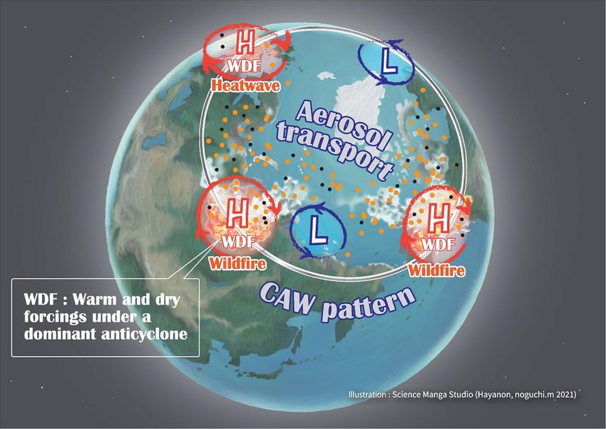
Environ. Res. Lett. 16 (2021) 064009 https://doi.org/10.1088/1748-9326/abf7ef
LETTER
Relationship between circum-Arctic atmospheric wave patterns
OPEN ACCESS
and large-scale wildfires in boreal summer
RECEIVED
12 October 2020 Teppei J Yasunari1,2,3,∗, Hisashi Nakamura4, Kyu-Myong Kim5, Nakbin Choi6, Myong-In Lee6,
REVISED Yoshihiro Tachibana7 and Arlindo M da Silva5
9 March 2021
1
Arctic Research Center, Hokkaido University, N21W11, Kita-ku, Sapporo, Hokkaido 001-0021, Japan
ACCEPTED FOR PUBLICATION 2
Global Station for Arctic Research, GI-CoRE, Hokkaido University, N21W11, Kita-ku, Sapporo, Hokkaido 001-0021, Japan
14 April 2021 3
Center for Natural Hazards Research, Hokkaido University, N9W9, Kita-ku, Sapporo, Hokkaido 060-8589, Japan
PUBLISHED 4
Research Center for Advanced Science and Technology, The University of Tokyo, 4-6-1 Komaba, Meguro-ku, Tokyo 153-8904, Japan
17 May 2021 5
NASA Goddard Space Flight Center, 8800 Greenbelt Road, Greenbelt, MD 20771, United States of America
6
Ulsan National Institute of Science and Technology, 50 UNIST-gil, Eonyang-eup, Ulju-gun, Ulsan 44919, Republic of Korea
Original content from 7
Faculty of Bioresources, Mie University, 1577 Kurimamachiya-cho, Tsu, Mie 514-8507, Japan
this work may be used ∗
Author to whom any correspondence should be addressed.
under the terms of the
Creative Commons E-mail: t.j.yasunari@arc.hokudai.ac.jp
Attribution 4.0 licence.
Any further distribution Keywords: wildfire, aerosol, PM2.5 , summer, Arctic, climate pattern, atmospheric circulation
of this work must
maintain attribution to
Supplementary material for this article is available online
the author(s) and the title
of the work, journal
citation and DOI.
Abstract
Long-term assessment of severe wildfires and associated air pollution and related climate patterns
in and around the Arctic is essential for assessing healthy human life status. To examine the
relationships, we analyzed the National Aeronautics and Space Administration (NASA)
modern-era retrospective analysis for research and applications, version 2 (MERRA-2). Our
investigation based on this state-of-the-art atmospheric reanalysis data reveals that 13 out of the
20 months with the highest PM2.5 (corresponding to the highly elevated organic carbon in the
particulate organic matter [POM] form) monthly mean mass concentration over the Arctic for
2003–2017 were all in summer (July and August), during which POM of ⩾0.5 µg m−3 and PM2.5
were positively correlated. This correlation suggests that high PM2.5 in the Arctic is linked to large
wildfire contributions and characterized by significant anticyclonic anomalies (i.e. clockwise
atmospheric circulation) with anomalous surface warmth and drier conditions over Siberia and
subpolar North America, in addition to Europe. A similar climate pattern was also identified
through an independent regression analysis for the July and August mean data between the same
atmospheric variables and the sign-reversed Scandinavian pattern index. We named this pattern of
recent atmospheric circulation anomalies the circum-Arctic wave (CAW) pattern as a
manifestation of eastward group-velocity propagation of stationary Rossby waves (i.e. large-scale
atmospheric waves). The CAW induces concomitant development of warm anticyclonic anomalies
over Europe, Siberia, Alaska, and Canada, as observed in late June 2019. Surprisingly, the extended
regression analysis of the 1980–2017 period revealed that the CAW pattern was not prominent
before 2003. Understanding the CAW pattern under future climate change and global warming
would lead to better prediction of co-occurrences of European heatwaves and large-scale wildfires
with air pollution over Siberia, Alaska, and Canada in and around the Arctic in summer.
1. Introduction June and July 2019, European heatwaves coincided
with large-scale wildfires over Siberia and Alaska
Global concern over wildfires has increased under (Nature 2019). Based on atmospheric and climate
the ongoing global warming (e.g. Running 2006, data provided by the Tokyo Climate Center (WMO
Jolly et al 2015, Veira et al 2016). In two recent years regional climate center in RA II), large areas of
(2019 and 2020), unprecedented wildfires occurred the extratropical Northern Hemisphere, including
in the Arctic and its vicinity (Witze 2020). During Europe, Siberia, and Alaska, were suffered from
© 2021 The Author(s). Published by IOP Publishing Ltd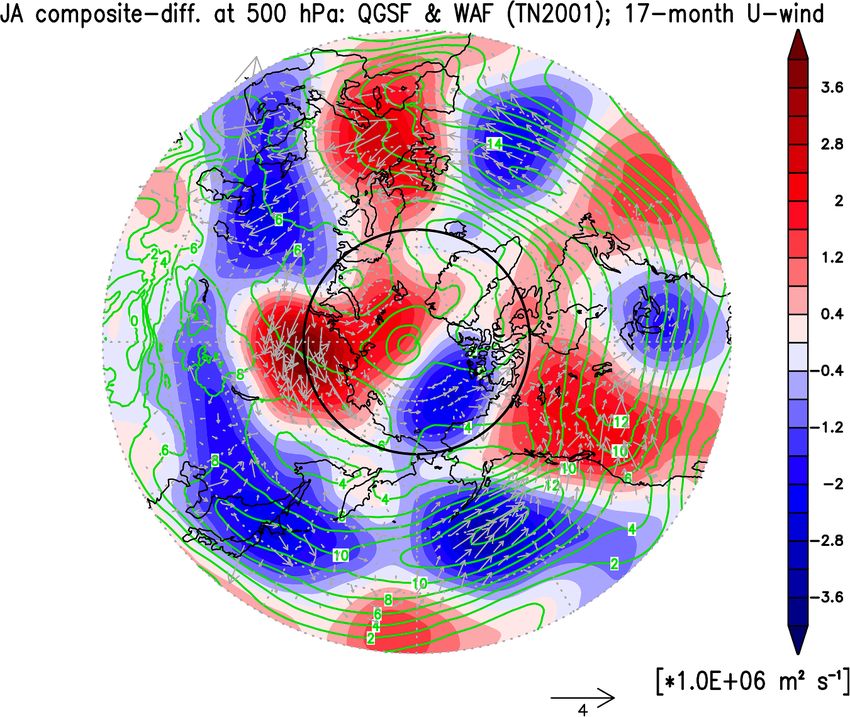
Environ. Res. Lett. 16 (2021) 064009                                                                 T J Yasunari et al

marked co-occurrences of extremely high temper-             and Mölders 2011). Therefore, there is still a lack of
ature during June and August 2019 (https://ds.dat           statistical research on air pollution, specifically on
a.jma.go.jp/tcc/tcc/products/climate/seasonal/season        PM2.5 , and capturing long-term variability in PM2.5
al_201906201908e.html) with heatwaves over                  in the Arctic has thus far been difficult in the absence
Europe during June and July (https://ds.da                  of continuous and extensive PM2.5 measurements.
ta.jma.go.jp/tcc/tcc/products/climate/annual/annual         Our understanding of long-term PM2.5 variation, air
_2019e.html). Severe and extensive wildfires across         quality in the Arctic and its surrounding areas, and
Alaska in June and July 2019 (see the satellite image       their linkage to variations in climatic conditions, such
at NASA’s worldview for 9 July 2019, at: https://           as anomalous atmospheric circulation, is therefore
go.nasa.gov/3n6PlUq) and Siberia (www.nasa.gov/             still limited.
image-feature/goddard/2019/siberian-smoke-headin                 Recently, the National Aeronautics and Space
g-towards-us-and-canada) also emitted air pollutants        Administration (NASA) produced MERRA-2
that were transported into distant areas. Character-        (Modern-Era Retrospective analysis for Research and
ized by atmospheric blacking, the Siberian wildfire in      Applications, Version 2), a long-term global reana-
the summer of 2019 caused extensive air pollution,          lysis dataset for atmospheric and other conditions
including PM2.5, which exceeded the 2011–2019 aver-         such as land and ocean (Bosilovich et al 2015). The
age values (Bondur et al 2020). It has been reported        best quality aerosol-related variables since 2003 in
that wildfires in and around Siberia have signific-         MERRA-2 are available because the most available
ant impacts not only on nearby areas but also on            satellite measurements were merged into the modeled
remote locations, such as Hokkaido in Japan, which          data for this period (Randles et al 2017). We, there-
has recorded considerable PM2.5 increases (Ikeda            fore, utilize the MERRA-2 reanalysis data in this
and Tanimoto 2015, Yasunari et al 2018), and the            study.
Arctic (Sitnov et al 2020). The above studies suggest            Thus far, case studies for Siberian wildfires and
meaningful connections among wildfires, aerosols            associated air pollution in and around the Arctic have
(air pollution), and climate patterns in and around         been reported (Ikeda and Tanimoto 2015, Yasunari
the Arctic region in recent years.                          et al 2018, Sitnov et al 2020). However, a number
    Aerosols over the Arctic region contribute to the       of questions remained unanswered. To address this
so-called Arctic haze (i.e. haze typically seen in spring   knowledge gap, we focused on three key factors in this
in the Arctic; Shaw 1995, Quinn et al 2007) and             study: (a) statistical relationships among wildfires,
affect cloud properties and radiative forcing (Zhao         PM2.5 , and wildfire-related aerosols, especially under
and Garrett 2015). Fractions of carbonaceous aer-           high air pollution (i.e. PM2.5 ) conditions, (b) identi-
osols such as black carbon (BC) and organic car-            fying the dominant climate pattern under high PM2.5
bon (OC) can increase owing to wildfires emissions          conditions in the Arctic, and (c) identifying whether
(e.g. Bond et al 2004, Wang et al 2011, Noguchi et al       this pattern has occurred only in recent years. The
2015). Another consequence of wildfires is the snow-        state-of-the-art MERRA-2 reanalysis data allowed us
darkening effect (SDE), which is due to reductions          to reveal the relationships among wildfires, aerosols
in snow albedo caused by the depositions of light-          (air pollution), and climate patterns in and around
absorbing aerosols such as BC, OC, and dust (War-           the Arctic. The outcome of this study provides a
ren and Wiscombe 1980, Flanner et al 2007, 2009,            resource to aid in making better forecasts in future
Yasunari et al 2010, 2011, Aoki et al 2011, Yasunari        studies.
et al 2013, 2014, 2015, Qian et al 2015, Lau et al
2018, Hock et al 2019). Solar forcing by SDE due to         2. Data and methods
post-wildfires has increased in the western US burned
forests since 1999 (Gleason et al 2019). A recent           2.1. Data
study revealed that surface melting on the Greenland        To examine recent temporal variations of air pollut-
ice sheet is accelerated during warmer-than-normal          ants in the Arctic, we used the monthly MERRA-2
summers because of high temperatures and increased          reanalysis data from January 2003 to December
BC deposition from wildfires (Keegan et al 2014).           2017 (15 years) for the global atmosphere based
Therefore, in addition to the essential connections         on the GEOS-5 model (Rienecker et al 2008),
with climate patterns, wildfire-generated aerosols are      including the data assimilation with observa-
also of significant concern for climate and snow-           tions since 1980 (Bosilovich et al 2015, Randles
darkening interactions.                                     et al 2017; https://gmao.gsfc.nasa.gov/reanalysis/
    However, many studies have often focused on             MERRA-2/). The MERRA-2 atmospheric data from
individual aerosol constituents that make up PM2.5 ,        1980 to 2017 was also used for some additional
rather than assessments of comprehensive air pollu-         analysis. The advantage of using MERRA-2 is that
tion (e.g. Sharma et al 2004, Eleftheriadis et al 2009,     observed aerosol optical depth (AOD) data from
Hegg et al 2009, Wang et al 2011, Yttri et al 2014) with    satellites and ground-based measurements (AER-
a few PM2.5 studies in and around the Arctic (Tran          ONET) are assimilated (Randles et al 2017). When

                                               2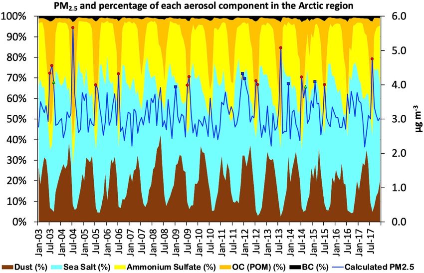
Environ. Res. Lett. 16 (2021) 064009                                                                T J Yasunari et al

observed AOD data are available, aerosol data simu-        PM2.5 months. Of which, 13, 5, and 2 months
lated in the GEOS-5 model are modified to reflect the      were found in summer (July 2003, August 2003,
observations (Randles et al 2017). The best aerosol        July 2004, July 2005, July 2006, July 2009, August
quality with lower bias was available in MERRA-2           2009, July 2012, August 2012, August 2013, July
from 2003 compared to that before 2003 (figure 5 of        2014, July 2015, and August 2017), winter (January
Randles et al 2017). MERRA-2 uses the monthly-             2009, December 2011, January 2012, December 2013,
mean quick fire emissions dataset (QFED) emis-             and February 2015), and fall (September 2003 and
sions (Darmenov and Da Silva 2015) up to 2010              September 2014), respectively (figure 1). Thus, the
and daily QFED emissions afterward. While daily            remainder of the study focused on the summer
biomass burning (BB) emissions are critical for cap-       months. These 13 summer months were then com-
turing day-to-day BB emission variability, the switch      pared with the other 17 summer months (July and
to daily BB emissions in 2010 does not introduce any       August) with the lower PM2.5 levels through compos-
long-term trends because the same monthly-mean             ite analysis shown later. Welch’s t-test (Welch 1938)
emissions were used before and after 2010. Notice          was used to assess the significant mean differences
that despite the fact that monthly mean BB emissions       in the composites. Most composites adopted a two-
were used prior to 2010, MERRA-2 can still capture         sided t-test for rejecting the null hypothesis, except
daily variability in BB aerosols due to the three-hourly   for those presented in SI figure S2 and SI table S1 (see
assimilation of aerosol data. Therefore, the switch to     supplementary information: SI (available online at
daily QFED emissions in 2010 should have minimal           stacks.iop.org/ERL/16/064009/mmedia)). For these
impacts on the analysis presented in this study. In        SI materials, we only would like to verify whether the
the GEOS-5 model, the original air pollutants (i.e.        PM2.5 and aerosol mass concentrations over Siberia,
aerosols) are simulated with the goddard chemistry         Alaska, and Canada for the high PM2.5 months in the
aerosol radiation and transport (GOCART) module            Arctic are higher than those for the other months.
(Chin et al 2000, Ginoux et al 2001, Chin et al 2002).     Therefore, we only focused on the positive (i.e.
In GOCART, OC is treated as Particulate Organic            increase) difference and thus used a one-sided t-test
Matter (POM = 1.4 × OC; Colarco et al 2010). This          for them (i.e. under the alternative hypothesis).
POM (OC in MERRA-2) is a good indicator of air                 The climate pattern’s essential dynamic pro-
pollution from wildfires (e.g. Yasunari et al 2018).       cesses can be illustrated with a particular form
The MERRA-2 aerosols have been validated region-           of a Rossby wave-activity flux (WAF) (Takaya and
ally and globally in recent studies (e.g. Buchard et al    Nakamura 2001), parallel to the group velocity of
2017, Yasunari et al 2017, 2018, He et al 2019, Sun        stationary Rossby waves (i.e. large-scale atmospheric
et al 2019, Gueymard and Yang 2020, Ma et al 2020).        waves). According to the linear theory, the flux mag-
Besides, a case study for the Siberian wildfire in 2016    nitude is proportional to the squared wave amp-
using MERRA-2, BC revealed long-range transport of         litude and the eastward group velocity. The latter
air pollution to the Arctic (Sitnov et al 2020), which     is proportional to the background westerly wind
further validated the usefulness of the MERRA-2 data       speed. The WAF of Takaya and Nakamura (2001)
in/around the Arctic region.                               was calculated with the modified script based on the
    We also used MODIS (moderate resolution ima-           GrADS script for WAF (http://www.atmos.rcast.u-
ging spectroradiometer) fire pixel counts (FPCs)           tokyo.ac.jp/nishii/programs/index.html).
retrieved by the Aqua satellite (available at: https://
feer.gsfc.nasa.gov/) to construct composites for 13        3. Results
high PM2.5 summer months. Monthly total FPCs
aggregated at 1◦ by 1◦ both in latitude and longitude      3.1. Characteristics of PM2.5 and aerosols, and their
are used to discuss a potential source of POM.             relationships with wildfire
    For our regression analysis, a known                   Here, we investigate monthly PM2.5 variations dur-
climate index of the Scandinavian pattern                  ing 2003–2017 by selecting 20 months with the
(www.cpc.ncep.noaa.gov/data/teledoc/scand.shtml)           worst air quality in the Arctic region. From the area-
was used; it was originally defined as the Eurasia type    mean data over the Arctic for 2003–2017 (figure 1),
1 pattern by Barnston and Livezey (1987).                  the fractions of dust, ammonium sulfate, sea salt,
                                                           BC, and OC (POM; hereafter called POM; pro-
2.2. Analytical techniques and statistics                  portional to OC in MERRA-2: see section 2) are
In this study, PM2.5 was calculated from the five          about 2.7%–42.5%, 9.5%–37.5%, 16.7%–73.1%,
MERRA-2 aerosol types in the PM2.5 size-dust,              0.5%–2.8%, and 1.5%–58.0% of the monthly mean
sulfate, BC, OC (i.e. POM), and sea salt—by the            Arctic PM2.5 , respectively. Generally, the dust con-
method (equation (1)) of Buchard et al (2016), in          tribution tends to be smaller in summer and fall but
which sulfate is assumed to be ammonium sulfate.           more prominent in spring. Sulfate aerosols are also
Monthly-mean values of area-averaged PM2.5 within          smaller in summer. Meanwhile, BC and POM peaked
the Arctic circle (at 66.56◦ N) were computed for          during summer, with the summer fractions reaching
15 years (2003–2017) before choosing the 20 highest        1.0%–2.8% and 13.8%–58.0%, respectively. These

                                              3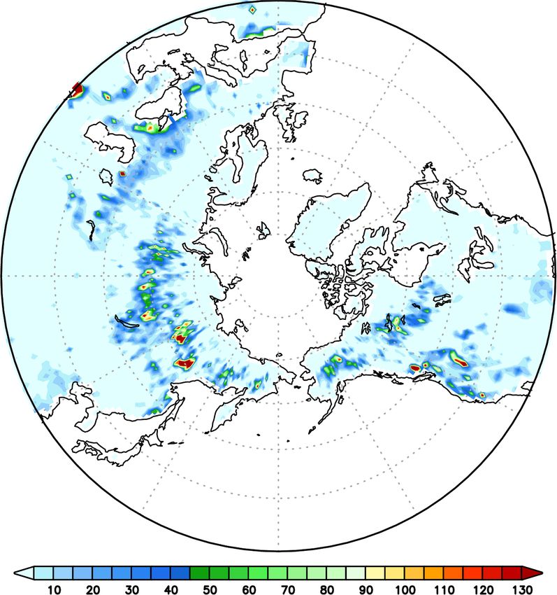
Environ. Res. Lett. 16 (2021) 064009                                                                                          T J Yasunari et al

   Figure 1. Time evolution of monthly-mean PM2.5 concentrations (µg m−3 ) (right) in the Arctic region and the fractional
   contributions in percentage (left) of individual aerosol species between 2003 and 2017 based on MERRA-2 data. Red circles, blue
   squares, and green triangles represent summer, winter, and fall, respectively, covering the 20 months of worst air quality (highest
   PM2.5 ) in the Arctic. Individual aerosol species include dust, sea salt, ammonium sulfate, (OC; POM), and BC, as detailed in the
   bottom legend.

   Figure 2. Comparison of calculated MERRA-2 PM2.5 and organic carbon (OC; particulate organic matter [POM]) mass
   concentration in the Arctic from 2003 to 2017. All data are monthly mean values averaged within the Arctic. Light orange circles
   denote all the data during the period. Blue circles indicate the monthly mean OC (POM) mass concentrations equal to or higher
   than 0.5 µg m−3 . Red circles represent the 13 summer months (July and August) among the 20 months with the highest PM2.5 in
   the Arctic (see figure 1 and section 2.2). The blue line is the linear regression for the blue circle data with its equation and R2 value.

findings imply a common emission source in sum-                           goes below approximately 16.7%, and the minimum
mer. Sea salt markedly increases in fall but decreases                    contribution is higher than the other aerosol
to a minimum, mainly in spring; its fraction never                        constituents.

                                                          4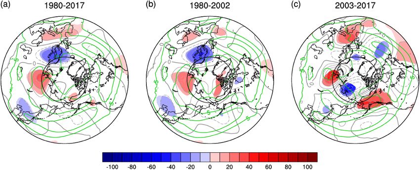
Environ. Res. Lett. 16 (2021) 064009 T J Yasunari et al
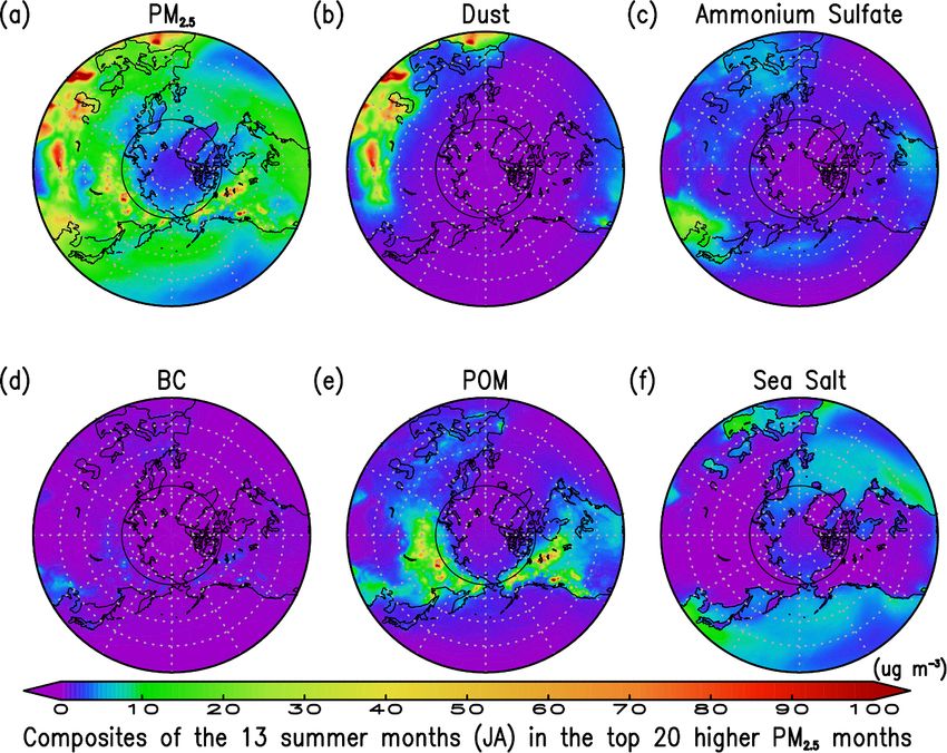
Figure 3. Composites of (a) PM2.5 levels for the 13 summer months (July and August) among the 20 months with the highest
PM2.5 between 2003 and 2017, and the corresponding mass concentrations of (b) dust, (c) ammonium sulfate, (d) BC, (e) POM
(see section 2.1), and (f) sea salt. All the units are in µg m−3 .
Of the 20 months of the worst air quality based on 3.2. Summer climate pattern under high PM2.5
PM2.5 , 13 months were in summer (figure 1). These conditions in the Arctic
13 significantly high PM2.5 months in summer also During the 13 highest PM2.5 months in summer (i.e.
correspond to higher POM months for 2003–2017 July and August), significant anticyclonic anomalies
(figure 2). When the Arctic-averaged monthly-mean (i.e. clockwise atmospheric circulation) from the
POM is not less than 0.5 µg m−3 , POM and PM2.5 lower (850 hPa) to mid-troposphere (500 hPa) were
were well explained by its strong linear relationship identified (figures 5(b) and (c)) over central Siberia
(R2 = 0.77). Those 13 high PM2.5 months in the and western Canada. The local PM2.5 and POM mass
Arctic summer were also characterized by region- concentrations over the regions were significantly
ally high POM (figure 3(a)). The POM mass con- high (figures 3(a), (e); SI figures S1 and S2; SI table S1)
centrations were greater over Siberia, Alaska, and owing to active wildfires (figure 4). These anticyclonic
Canada (figure 3(e)), where wildfires were very act- anomalies tend to accompany anomalous high sur-
ive (figure 4). The POM increased significantly in the face air temperatures (figure 5(a)) that are significant
13 summer months (July and August) in Siberia and over Siberia and Canada in July and August, as well
Canada compared with the other July and August as significantly drier conditions over Siberia, Alaska,
months, where increased BC was also prominent (SI and Canada (SI figure S3). The anomaly pattern in
figures S1 and S2; SI table S1). The POM increase in figure 5 also resembles the warm anticyclonic anom-
Alaska was significant only in July (SI table S1). Those alies observed over western Europe, central Siberia,
results indicate that the 13 highest PM2.5 months in Alaska, and Canada in late June 2019 (SI figure S4).
summer (July and August) in the Arctic in 2003–2017 Figure 6 shows WAF in the atmosphere evaluated
were also higher POM months due to active wild- from the composite anomaly fields for the 13 summer
fires over Siberia and subpolar North America in and months and their differences in geostrophic stream
around the Arctic. Also, the POM increase tended to functions (from geopotential height) with the com-
be accompanied by BC increases from the same areas posite of horizontal winds for the 17 other summer
(figure 3(d)). months at 500 hPa. The warm anticyclonic anomalies
5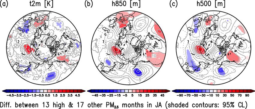
Environ. Res. Lett. 16 (2021) 064009                                                                             T J Yasunari et al

   Figure 4. Composite of monthly mean MODIS FPCs (unit: count per 1◦ latitude × 1◦ longitude grid) retrieved by the Aqua
   satellite (available at: https://feer.gsfc.nasa.gov/) for the 13 summer months (July and August) with the highest PM2.5
   concentrations in the Arctic.

are accompanied by two eastward-developing Rossby                 scand.shtml). Regression maps between the sign-
wave trains along the westerly jet stream, one from               reversed July and August mean Scandinavian pat-
Europe to Alaska via Siberia and the other from                   tern index and the three meteorological variables
the North Pacific to Alaska (see the vectors in                   (figure 7) show a very similar climate pattern in
figure 6).                                                        the atmosphere obtained from the composite dif-
                                                                  ferences (figure 5). Positive anticyclonic anomalies
3.3. Regression analysis with the scandinavian                    at 850 and 500 hPa over Europe, Siberia, and sub-
pattern index                                                     polar North America (Alaska and Canada) were evid-
We further performed an independent regression                    ent, corresponding to the near-surface warm anom-
analysis with the same three meteorological variables             alies (figures 5 and 7). These relationships imply
used in figure 5. Here we use the Scandinavian                    that the climate pattern that characterizes the 13
pattern index; a known climate pattern origin-                    highest PM2.5 summer months in the Arctic by the
ally referred to as the Eurasia-1 pattern (Barnston               composite analysis (figure 5) is well explained by
and Livezey 1987). The index is valid for assess-                 the inter-annual variations of the sign-reversed July
ing unusual climate such as blocking, temperature                 and August mean Scandinavian pattern index for the
anomalies, etc, over Eurasia from Scandinavia to                  2003–2017 period. To emphasize the characteristic of
East Eurasia (www.cpc.ncep.noaa.gov/data/teledoc/                 pressure anomalies aligned zonally around the Arctic

                                                    6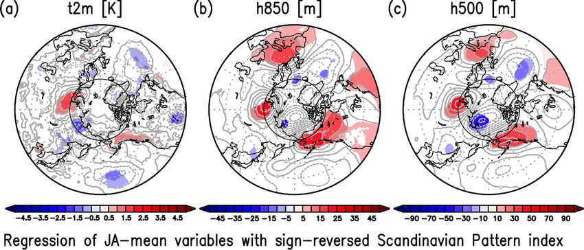
Environ. Res. Lett. 16 (2021) 064009                                                                                    T J Yasunari et al

   Figure 5. Composited differences (solid contours) in (a) surface air temperature (0.5 K intervals) and (b) geopotential height at
   850 hPa (5 m intervals) and (c) 500 hPa (10 m intervals) between the 13 summer months (July and August) of 20 months with the
   highest PM2.5 concentrations in the Arctic region, and the 17 other summer months. Local anomalies that exceed the 95%
   confidence level based on Welch’s t-test (two-sided; see section 2.2) are shown in shaded contours.

   Figure 6. WAF calculated by Takaya and Nakamura (2001) and quasi-geostrophic stream function (shaded contour; see the color
   bar with the unit shown in the figure) of the composite difference among the 13 summer months of the 20 months with the
   highest PM2.5 and the other 17 summer months (i.e. low PM2.5 ), and the composite of U-wind for the 17 other summer months
   under the basic PM2.5 state (westerly wind in green contour at 1 m s−1 interval) at 500 hPa. For WAF (vector in the unit of
   m2 s−2 ), data are plotted at every ten (north of 60◦ N) and eight (south of 60◦ N) grid points in the meridional direction, and
   every five grid points in a longitudinal direction. Besides, we only considered the magnitudes of the basic state of UV-wind equal
   to or greater than 5 m s−1 for plotting the WAF.

                                                       7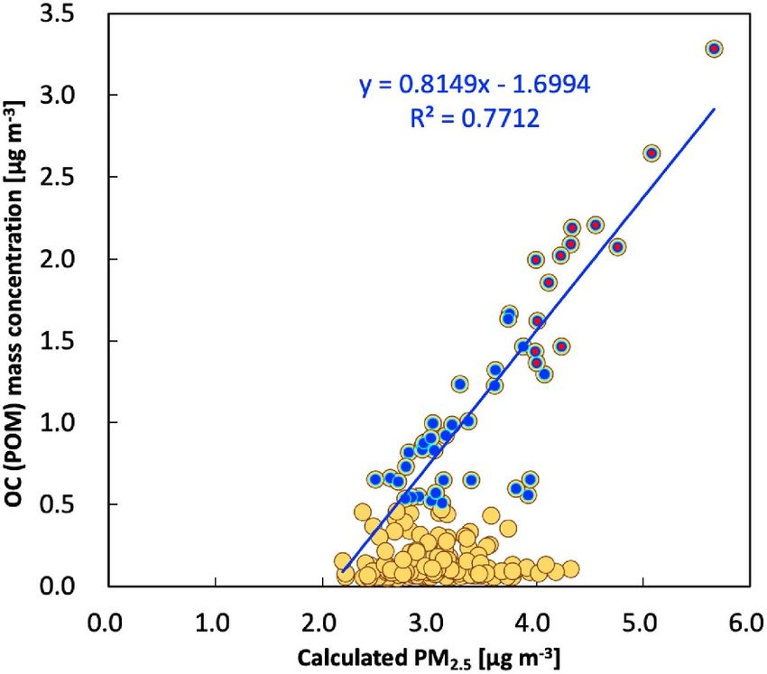
Environ. Res. Lett. 16 (2021) 064009                                                                                   T J Yasunari et al

   Figure 7. Mean anomalies (solid contours) of July and August (a) surface air temperature (0.5 K intervals), (b) geopotential
   height at 850 hPa (5 m intervals), and (c) 500 hPa (10 m intervals) regressed against the sign-reversed July and August mean
   Scandinavian pattern index (see section 2.1). Local anomalies that exceed the 95% confidence level based on t-test (two-sided; see
   section 2.2) are shown in shaded contours.

   Figure 8. ‘Negative’ Scandinavian pattern teleconnection pattern for (a) 1980–2017, (b) 1980–2002, and (c) 2003–2017 obtained
   from the regression of 500 hPa geopotential height anomalies (July and August means) onto the ‘negative’ (sign-reversed)
   Scandinavian pattern index. The solid green line denotes the U-wind climatology (i.e. westerly wind) at 500 hPa for each period
   (plots starting from 5 m s−1 with a 5 m s−1 interval). Shaded areas indicate 95% statistical confidence.

from Europe to Siberia, Alaska, Canada, and back to                  forming the CAW. The CAW-associated positive anti-
Europe, we refer to this summertime climate pattern                  cyclonic (geopotential height) anomalies at 500 hPa
as the circum-Arctic wave (CAW) pattern.                             over Europe and Siberia are also stronger than their
    However, if we performed the same regres-                        counterpart associated with the Scandinavian pattern
sion analysis extended for a long-term period (i.e.                  before 2003. This change would imply a possible shift
including 1980–2002), the climate pattern only                       of the summertime climate pattern (teleconnection
shows a NW–SE oriented (line-shaped) atmospheric                     pattern; i.e. climate links between remote regions)
teleconnection pattern from Scandinavia to East Asia                 before and after 2003 and forming the co-occurrence
(figure 8(b)) rather than the CAW. This pattern                      of warm surface anomalies over Europe, Siberia,
resembles a typical Scandinavian pattern, as repor-                  Alaska, and Canada in CAW (figures 5 and 7).
ted in Bueh and Nakamura (2007), although they
excluded the summer season from their analysis. This                 4. Discussion and conclusions
climate pattern exclusively identified over Eurasia is
also dominant in the regression for the whole period                 We have found high PM2.5 mass concentrations over
(1980–2017; figure 8(a)). This characteristic indic-                 the summertime Arctic in 2003–2017 (figure 1).
ates that the typical Scandinavian pattern was dom-                  These high PM2.5 months also correspond to higher
inant over Eurasia before 2003, and afterward, the                   POM (figure 2) and its significant increase over
climate pattern has somehow been modified into                       Siberia and Canada (SI figures S1 and S2; POM in

                                                       8
Environ. Res. Lett. 16 (2021) 064009 T J Yasunari et al
Alaska only significant in July: SI table S1), where Nakamura 2007), the recent summertime Scand-
wildfires were very active (figure 4). OC (also BC) is inavian pattern or CAW (figure 7(c)) accompanies
a good indicator of wildfire activity (BB; e.g. Bond anticyclonic anomalies from Europe to Alaska along
et al 2004, Spracklen et al 2007, Noguchi et al 2015, the subpolar westerly jet stream that forms in July
Yasunari et al 2018, Shikwambana 2019). Therefore, and August along the Siberian coast (Nakamura and
we argue that the significantly increasing contribu- Fukamachi 2004, Tachibana et al 2004). Notably, a
tions of organic aerosols to Arctic PM2.5 are mainly similar anomaly pattern, which slightly shifted west-
due to wildfire smoke in and around the Arctic. This ward from the corresponding regression patterns
characteristic is consistent with results modeled from (figure 7), is also apparent in the pressure anomalies
October 1999 to May 2005 in a previous study (Stohl composited for the 13 summer months with the high
2006). In conclusion, for 2003–2017, the 13 higher PM2.5 (figure 5). As demonstrated by the WAF in the
PM2.5 months out of the 20 worst air quality months atmosphere (figure 6; Takaya and Nakamura 2001),
in the Arctic are explained by the greatly increased OC the CAW is likely a manifestation of eastward group-
(POM) with some BC increases from active wildfires velocity propagation of a stationary Rossby wave train
in Siberia, Alaska, and Canada. from Europe to Alaska along the upper-troposphere
We have also examined the causes for summers westerly jet stream. The CAW is also associated with
when the Arctic air quality worsens with domin- near-surface warm and tropospheric dry anomalies,
ant climate patterns. Investigating those climatic pat- as shown in figure 7(a) and SI figure S3. Our analysis
terns involved in forming warm anticyclonic anom- substantiates the previously discussed importance of
alies over Siberia, Alaska, and Canada under the high mid-tropospheric anticyclonic circulations in wild-
PM2.5 conditions (i.e. worse air quality) in the Arctic fire occurrences in Siberia and Alaska (Hayasaka et al
is essential for better prediction of large-scale wild- 2016, 2019, Bondur et al 2020). Note that the similar-
fire occurrences in the future. For this purpose, com- ity between figures 5 and 7 was unexpected.
posite and regression analyses for 2003–2017 were A similar eastward-extending Rossby wavy pat-
performed (figures 5 and 7). The composite analysis tern along the subpolar jet stream was observed
extracted anticyclonic anomalies from the lower to in summer 2010, which induced extreme warm-
mid-troposphere over Europe, Siberia, and Canada ness, especially in eastern Europe, Russia, and Japan
(figures 5(b) and (c)), which locally caused anomal- (Otomi et al 2013). The particular wave train and
ous near-surface warmth and dryness from near the that associated the CAW both form along the sub-
surface to the lower troposphere (figure 5(a); SI figure polar jet stream over northern Eurasia in association
S3). A recent study with the MODIS fire and MERRA with the enhanced poleward temperature gradient in
reanalysis (the former product of MERRA-2) data summer between the warmer Eurasian continent and
concluded that the primary months of wildfire activ- the cooler Arctic (Serreze et al 2001, Nakamura and
ity in the circumpolar Arctic tundra region were July Fukamachi 2004, Tachibana et al 2010).
and August, and those occurred under warm and dry Interestingly, the CAW and associated anticyc-
conditions (Masrur et al 2018). Their results strongly lonic anomalies over Europe, Siberia, and subpolar
support our results. The extreme anomalous warmth North America became prominent only from 2003
is also likely to induce heatwaves (Chase et al 2006, (figure 8). Amplified anomalies in recent years over
Feudale and Shukla 2011); the associated abnormal Alaska and western Canada can be explained by con-
dryness favors active wildfires (Bondur 2011). Our verging WAF. Those were associated with the wave
composited climate pattern in summer (figure 5) is trains (the one from Siberia via the Arctic Ocean; the
likely to set a favorable condition for heatwaves over other from the North Pacific) if the composite dif-
Europe and active wildfires (figure 4) over Siberia, ference pattern in figure 5 and the ‘negative’ Scand-
Alaska, and Canada, causing high PM2.5 and POM inavian pattern in figure 7 have a similar mechan-
and BC emissions in and around the Arctic. ism (figure 6). Elucidating the CAW formation is
To elucidate the relationship between the climate beyond the scope of this work but should focus on
patterns of recent years (2013–2017) and the long- future studies. A recent numerical simulation showed
term, we focused on the Scandinavian pattern as that a response to a heat source prescribed in west-
a well-known climate pattern. A recent paper also ern Russia could be similar to the Scandinavian pat-
reported that the Scandinavian pattern is relevant to tern over Siberia (Choi et al 2020). Their results may
the summer heatwave activity after the mid-1990s explain the summer CAW observed in the recent years
(Choi et al 2020), substantiating this index’s useful- (figure 7(c)), resulting in co-occurrences of heatwaves
ness for our analysis. As illustrated in the regression over Europe and large-scale wildfires in Siberia and
patterns in figure 7, the negative phase (i.e. sign- subpolar North America, notably Alaska and Canada
reversed index) of the Scandinavian pattern is char- (figures 4, 5(a) and 7(a)).
acterized by mid-tropospheric anticyclonic anom- Therefore, it is not surprising to observe a quasi-
alies in Europe, central Siberia, Alaska, and Canada. stationary wave train in late June 2019, similar to the
Unlike its counterpart in the cold season (Bueh and CAW as a recent example (SI figure S4). This situation
9Environ. Res. Lett. 16 (2021) 064009 T J Yasunari et al
Figure 9. Schematic summary of the results obtained in this study. Anomalous anticyclones developed concomitantly in summer
(July and August) over the circumpolar regions: Europe, Siberia, and subpolar North America (i.e. Alaska and Canada). Those
anticyclones induce warm and dry forcings from the surface to the mid-troposphere. This study names this climate pattern the
CAW pattern. Those anomalous anticyclones induce heatwaves over Europe and active wildfires over Siberia and subpolar North
America. The wildfire smoke emitted OC and BC aerosols into the atmosphere, and those aerosols could reach the Arctic region
to increase PM2.5 there. The interactions between the CAW pattern and the atmospheric aerosols must be investigated in future
studies. Reproduced from Hayanon Science Manga Studio. CC BY 3.0.
likely induced the concomitant occurrence of a heat- Arctic, acting to lower air quality (figure 2). The inter-
wave in Europe, and the Siberian and Alaskan wild- action between the aerosols and CAW may be pos-
fires, as mentioned in section 1. The climatic impacts sible through the impact of carbonaceous aerosols
of the Scandinavian pattern during fall, winter, and on climate via radiative effects (e.g. Liu et al 2014,
spring have been well explored (Blackburn and Zhang et al 2017). However, we have presented no
Hoskins 2001, Bueh and Nakamura 2007, Pall et al solid evidence to substantiate this interaction. There-
2011). However, a recent study (Choi et al 2020) and fore, further investigation is needed in the future.
this study have only emphasized the importance of Our study reveals the climatic significance of the
the corresponding summertime pattern on heatwaves recent July and August mean Scandinavian pattern,
and related large-scale wildfires. particularly its ‘negative phase’ (i.e. CAW pattern).
A schematic in figure 9 summarizes all the As a stationary atmospheric Rossby wave train with
possible connections from the unique circumpolar fast eastward group velocity (figure 6), the CAW
atmospheric circulation pattern in summer, CAW, can act as a useful dynamic indicator in summer
which has become predominant since 2003, to highly of the simultaneous occurrences of heatwaves in
increased aerosols in the Arctic. The CAW pattern can Europe, Siberia, Alaska, and Canada, and also works
induce the anomalous warmth (figure 7(a)) and dry- to increase the probability of large-scale wildfires
ness near the surface and in the lower troposphere in Siberia, Alaska, and Canada, and thereby higher
(figure S3) under anomalous high-pressure systems PM2.5 and OC (POM) concentrations in the Arctic. A
(figures 7(b) and (c)). The anomalous anticyclones recent study reported the relationships among wild-
are likely to cause heatwave over Europe and wildfire fire activity in the Arctic tundra and meteorological
occurrences in Siberia and subpolar North America variables (Masrur et al 2018). In conjunction with
(Alaska and Canada) (figure 4) with massive aerosol that study, this study further provides perspectives on
injections such as POM and BC into the atmosphere their connections to wildfire-induced air pollution
(figure 3; SI figures S1 and S2; SI table S1). The and spatiotemporal climate pattern. As increasing
CAW-associated atmospheric circulation can eventu- wildfires projected under global warming have been
ally transport the wildfire-induced aerosols into the discussed (Veira et al 2016), further investigations are
10Environ. Res. Lett. 16 (2021) 064009 T J Yasunari et al
required to deepen our understanding of the sum- Hisashi Nakamura https://orcid.org/0000-0003-
mertime CAW pattern. The trigger mechanism and 1791-6325
its persistence under such climate conditions as sea- Kyu-Myong Kim https://orcid.org/0000-0002-
surface temperature anomalies are yet to be explored. 3857-2085
It is also essential to assess whether the CAW will Nakbin Choi https://orcid.org/0000-0002-8696-
likely emerge throughout the extended summer sea- 5916
son under the warming climate. A better projection Myong-In Lee https://orcid.org/0000-0001-8983-
of this will help take effective measures of large-scale 8624
summer heatwaves and severe wildfires that lead to Yoshihiro Tachibana https://orcid.org/0000-0002-
massive air pollutants in and around the Arctic. 9194-3375
Arlindo M da Silva https://orcid.org/0000-0002-
Data availability 3381-4030
The data used in this study are available from the
corresponding author or co-authors upon reasonable
References
request. MERRA-2 and fire data from MODIS are Aoki T, Kuchiki K, Niwano M, Kodama Y, Hosaka M and
also publicly available at: https://gmao.gsfc.nasa.gov/ Tanaka T 2011 J. Geophys. Res. 116 D11114
reanalysis/MERRA-2/; https://feer.gsfc.nasa.gov/ Barnston A G and Livezey R E 1987 Mon. Weather Rev.
index.php. 115 1083–126
Blackburn M and Hoskins B J 2001 Department of Meteorology,
The data that support the findings of this study are University of Reading (available at: www.met.rdg.ac.uk/
available upon reasonable request from the authors. ∼mike/autumn2000/son00_paper9.pdf) (Accessed 2 March
2021)
Bond T C, Streets D G, Yarbe K F, Nelson S M, Woo J-H and
Acknowledgments Klimont Z 2004 J. Geophys. Res. 109 D14203
Bondur V G 2011 Izv. Atmos. Ocean. Phys. 47 1039–48
Bondur V G, Mokhov I I, Voronova O S and Sitnov S A 2020 Dokl.
We want to thank two anonymous reviewers for Earth Sci. 492 370–5
their helpful comments in revising the paper. This Bosilovich M G et al 2015 NASA/TM–2015–104606 vol
study is supported in part by the Japanese Ministry 43 (available at: https://gmao.gsfc.nasa.gov/pubs/docs/
Bosilovich803.pdf) (Accessed 2 March 2021)
of Education, Culture, Sports, Science and Tech- Buchard V et al 2017 J. Clim. 30 6851–72
nology through the Arctic Challenge for Sustain- Buchard V, Da Silva A M, Randles C A, Colarco P, Ferrare R,
ability (ArCS; JPMXD1300000000) project and its Hair J, Hostetler C, Tackett J and Winker D 2016 Atmos.
successor project (ArCS II; JPMXD1420318865), Environ. 125 100–11
Bueh C and Nakamura H 2007 Q. J. R. Meteorol. Soc.
and by the Japan Society for the Promotion of 133 2117–31
Science through the Grants-in-Aid for Scientific Chase T N, Wolter K, Pielke R A and Rasool I 2006 Geophys. Res.
Research (JSPS KAKENHI 17H02958, 17KT0066, Lett. 33 L23709
18H01278, 19H01976, 19H05668, 19H05698, Chin M, Ginoux P, Kinne S, Torres O, Holben B N, Duncan B N,
Martin R V, Logan J A, Higurashi A and Nakajima T 2002
19H05702, 20H01970, and 20K12197) and by the J. Atmos. Sci. 59 461–83
Japanese Ministry of Environment through Environ- Chin M, Rood R B, Lin S-J, Müller J-F and Thompson A M 2000
ment Research and Technology Development Fund J. Geophys. Res. 105 24671–87
JPMEERF20192004. NASA’s Global Modelling and Choi N, Lee M-I, Cha D-H, Lim Y-K and Kim K-M 2020 J. Clim.
33 1505–22
Assimilation Office (GMAO) produced the MERRA- Colarco P, Da Silva A, Chin M and Diehl T 2010 J. Geophys. Res.
2 reanalysis data, and we also used NCCS for data 115 D14207
analyses. We also thank NASA’s MODIS team for Darmenov A and Da Silva A 2015 NASA/TM–2015–104606 vol
making the fire pixel count data available. Shunsuke 38 (available at: https://gmao.gsfc.nasa.gov/pubs/docs/
Darmenov796.pdf) (Accessed 2 March 2021)
Tei (Forestry and Forest Products Research Institute) Eleftheriadis K, Vratolis S and Nyeki S 2009 Geophys. Res. Lett.
provided a helpful discussion of the calculations of 36 L02809
PM2.5 and aerosol composite differences (statistics). Feudale L and Shukla J 2011 Clim. Dyn. 36 1691–703
Kazuaki Nishii (Mie University) helped with plot- Flanner M G, Zender C S, Hess P G, Mahowald N M, Painter T H,
Ramanathan V and Rasch P J 2009 Atmos. Chem. Phys.
ting the WAF with the GrADS script. We want to 9 2481–97
thank Editage (www.editage.com) for English lan- Flanner M G, Zender C S, Randerson J T and Rasch P J 2007 J.
guage editing before the initial submission. We appre- Geophys. Res. 112 D11202
ciate Science Manga Studio (Hayanon, noguchi.m) Ginoux P, Chin M, Tegen I, Prospero J M, Holben B, Dubovik O
and Lin S J 2001 J. Geophys. Res. 106 20255–73
to make the schematic figure for summarizing our Gleason K E, Mcconnell J R, Arienzo M M, Chellman N and
results. Calvin W M 2019 Nat. Commun. 10 2026
Gueymard C A and Yang D 2020 Atmos. Environ.
ORCID iDs 225 117216
Hayasaka H, Tanaka H L and Bieniek P A 2016 Polar Sci.
10 217–26
Teppei J Yasunari https://orcid.org/0000-0002- Hayasaka H, Yamazaki K and Naito D 2019 J. Disaster Res.
9896-9404 14 641–8
11Environ. Res. Lett. 16 (2021) 064009 T J Yasunari et al
He L, Lin A, Chen X, Zhou H, Zhou Z and He P 2019 Remote Shaw G E 1995 Bull. Am. Meteorol. Soc. 76 2403–13
Sens. 11 460 Shikwambana L 2019 Remote Sens. Lett. 10 373–80
Hegg D A, Warren S G, Grenfell T C, Doherty S J, Larson T V and Sitnov S A, Mokhov I I and Likhosherstova A A 2020 Atmos. Res.
Clarke A D 2009 Environ. Sci. Technol. 43 4016–21 235 104763
Hock R G et al 2019 IPCC Special Report on the Ocean and Spracklen D V, Logan J A, Mickley L J, Park R J, Yevich R,
Cryosphere in a Changing Climate H-O Pörtner et al (eds) in Westerling A L and Jaffe D A 2007 Geophys. Res. Lett.
press (www.ipcc.ch/srocc/chapter/chapter-2/) (Accessed 2 34 L16816
March 2021) Stohl A 2006 J. Geophys. Res. 111 D11306
Ikeda K and Tanimoto H 2015 Environ. Res. Lett. 10 105001 Sun E, Xu X, Che H, Tang Z, Gui K, An L, Lu C and Shi G 2019
Jolly W M, Cochrane M A, Freeborn P H, Holden Z A, Brown T J, J. Atmos. Sol.-Terr. Phys. 186 8–19
Williamson G J and Bowman D M J S 2015 Nat. Commun. Tachibana Y, Iwamoto T, Ogi M and Watanabe Y 2004 J. Meteorol.
6 7537 Soc. Japan 82 1399–415
Keegan K M, Alber M R, Mcconnell J R and Baker I 2014 Proc. Tachibana Y, Nakamura T, Komiya H and Takahashi M 2010
Natl Acad. Sci. USA 111 7964–7 J. Geophys. Res. 115 D12125
Lau W K M, Sang J, Kim M K, Kim K M, Koster R D and Takaya K and Nakamura H 2001 J. Atmos. Sci. 58 608–27
Yasunari T J 2018 J. Geophys. Res. 123 8441–61 Tran H N Q and Mölders N 2011 Atmos. Res. 99 39–49
Liu Y, Goodrick S and Heilman W 2014 For. Ecol. Manage. Veira A, Lasslop G and Kloster S 2016 J. Geophys. Res.
317 80–96 121 3195–223
Ma J, Xu J and Qu Y 2020 Atmos. Environ. 237 117666 Wang Q et al 2011 Atmos. Chem. Phys. 11 12453–73
Masrur A, Petrov A N and DeGroote J 2018 Environ. Res. Lett. Warren S G and Wiscombe W J 1980 J. Atmos. Sci.
13 014019 37 2734–45
Nakamura H and Fukamachi T 2004 Q. J. R. Meteorol. Soc. Welch B L 1938 Biometrika 29 350–62
130 1213–33 Witze A 2020 Nature 585 336–7
Nature 2019 Nature 572 10–1 Yasunari T J et al 2017 SOLA 13 96–101
Noguchi I, Akiyama M, Suzuki H and Yamaguchi T 2015 Abstract Yasunari T J, Bonasoni P, Laj P, Fujita K, Vuillermoz E,
for the 2nd Atmospheric Aerosol Symp. from Kosa to Marinoni A, Cristofanelli P, Duchi R, Tartari G
PM2.5 —Environmental and Health Impacts p 2 and Lau K-M 2010 Atmos. Chem. Phys.
(in Japanese) 10 6603–15
Otomi Y, Tachibana Y and Nakamura T 2013 Clim. Dyn. Yasunari T J, Kim K-M, Da Silva A M, Hayasaki M, Akiyama M
40 1939–47 and Murao N 2018 Sci. Rep. 8 6413
Pall P, Aina T, Stone D A, Stott P A, Nozawa T, Hilberts A G J, Yasunari T J, Koster R D, Lau K-M, Aoki T, Sud Y C, Yamazaki T,
Lohmann D and Allen M R 2011 Nature 470 382–5 Motoyoshi H and Kodama Y 2011 J. Geophys. Res.
Qian Y, Yasunari T J, Doherty S J, Flanner M G, Lau W K M, 116 D02210
Ming J, Wang H, Wang M, Warren S G and Zhang R 2015 Yasunari T J, Koster R D, Lau W K M and Kim K M 2015
Adv. Atmos. Sci. 32 64–91 J. Geophys. Res. 120 5485–503
Quinn P K, Shaw G, Andrews E, Dutton E G, Ruoho-Airola T and Yasunari T J, Lau K-M, Mahanama S P P, Colarco P R, Da
Gong S L 2007 Tellus B 59 99–114 Silva A M D, Aoki T, Aoki K, Murao N, Yamagata S and
Randles C A et al 2017 J. Clim. 30 6823–50 Kodama Y 2014 SOLA 10 50–6
Rienecker M M et al 2008 Technical Report Series on Global Yasunari T J, Tan Q, Lau K-M, Bonasoni P, Marinoni A, Laj P,
Modeling and Data Assimilation vol 27 (available at: https:// Ménégoz M, Takemura T and Chin M 2013 Atmos. Environ.
gmao.gsfc.nasa.gov/pubs/docs/Rienecker369.pdf) (Accessed 78 259–67
2 March 2021) Yttri K E, Lund Myhre C, Eckhardt S, Fiebig M, Dye C,
Running S W 2006 Science 313 927–92 Hirdman D, Ström J, Klimont Z and Stohl A 2014 Atmos.
Serreze M C, Lynch A H and Clark M P 2001 J. Clim. 14 1550–67 Chem. Phys. 14 6427–42
Sharma S, Lavoué D, Cachier H, Barrie L A and Gong S L 2004 Zhang Y et al 2017 Nat. Geosci. 10 486–9
J. Geophys. Res. 109 D15203 Zhao C and Garrett T J 2015 Geophys. Res. Lett. 42 557–64
12You can also read