Spatio-Temporal Dynamics of Online Memes: A Study of Geo-Tagged Tweets
←
→
Page content transcription
If your browser does not render page correctly, please read the page content below
Spatio-Temporal Dynamics of Online Memes:
                        A Study of Geo-Tagged Tweets

                   Krishna Y. Kamath, James Caverlee, Kyumin Lee, and Zhiyuan Cheng
                          Department of Computer Science and Engineering, Texas A&M University
                                           College Station, TX, USA - 77843
                                {kykamath, caverlee, kyumin, zcheng}@cse.tamu.edu

ABSTRACT                                                             access to the fine-grained spatio-temporal logs of user activ-
We conduct a study of the spatio-temporal dynamics of                ities. For example, the Foursquare location sharing service
Twitter hashtags through a sample of 2 billion geo-tagged            has enabled 2 billion “check-ins” [12], whereby users can link
tweets. In our analysis, we (i) examine the impact of loca-          their presence, notes, and photographs to a particular venue.
tion, time, and distance on the adoption of hashtags, which          The mobile image sharing service Instagram allows users
is important for understanding meme diffusion and infor-             to selectively attach their latitude-longitude coordinates to
mation propagation; (ii) examine the spatial propagation             each photograph; similar geo-tagged image sharing services
of hashtags through their focus, entropy, and spread; and            are provided by Flickr and a host of other services. And
(iii) present two methods that leverage the spatio-temporal          the popular Twitter service sees ∼300 million Tweets per
propagation of hashtags to characterize locations. Based on          day, of which ∼3 million are tagged with latitude-longitude
this study, we find that although hashtags are a global phe-         coordinates.
nomenon, the physical distance between locations is a strong            Access to these geo-spatial footprints opens new oppor-
constraint on the adoption of hashtags, both in terms of the         tunities to investigate the spatio-temporal dynamics of on-
hashtags shared between locations and in the timing of when          line memes, which has important implications for a vari-
these hashtags are adopted. We find both spatial and tem-            ety of systems and applications, including targeted adver-
poral locality as most hashtags spread over small geograph-          tising, location-based services, social media search, and con-
ical areas but at high speeds. We also find that hashtags            tent delivery networks. Hence, in this paper, we initiate
are mostly a local phenomenon with long-tailed life spans.           a study of the spatio-temporal properties of social media
These (and other) findings have important implications for           spread through an examination of the fine-grained sharing of
a variety of systems and applications, including targeted ad-        one type of global-scale social media – a sample of 2 billion
vertising, location-based services, social media search, and         geo-tagged Tweets with precise latitude-longitude coordi-
content delivery networks.                                           nates collected over the course of 18 months. Specifically we
                                                                     consider the propagation of hashtags across Twitter, where a
                                                                     hashtag is a simple user-generated annotation prefixed with
Categories and Subject Descriptors                                   a #. Hashtags serve many purposes on Twitter, from as-
H.3.4 [Information Storage and Retrieval]: Systems                   sociating Tweets with particular events (e.g., #ripstevejobs
and Software—Information networks                                    and #fukushima) to sharing memes and conversations (e.g.,
                                                                     #bestsportsrivalry and #ifyouknowmeyouknow). Our goal
Keywords                                                             is to explore questions such as:
social media; spatial impact; spatio-temporal analysis
                                                                        • What role does distance play in the adoption of hash-
                                                                          tags? Does distance between two locations influence
1.    INTRODUCTION                                                        both what users in different locations adopt and when
   The rise of social media services enables a global-scale in-           they do so?
frastructure for the sharing of videos, blogs, images, tweets,
and other user-generated content. As users consume and                  • While social media is widely reported in terms of viral
share this content, some content may gain traction and be-                and global phenomenon, to what degree are hashtags
come popular resulting in viral videos and popular memes                  truly a global phenomenon?
that captivate the attention of huge numbers of users. These
phenomena have attracted a considerable amount of recent                • What are the geo-spatial properties of hashtag spread?
research to study the dynamics of the adoption of social me-              How do local and global hashtags differ?
dia, e.g., [4, 13, 15, 17, 20].
   Augmenting this rich body of research is the widespread              • How fast do hashtags peak after being introduced?
adoption of GPS-enabled tagging of social media content via               And what are the geo-spatial factors impacting the
smartphones and social media services, which provides new                 timing of this peak?
Copyright is held by the International World Wide Web Conference        • How can the spatio-temporal characteristics of hash-
Committee (IW3C2). IW3C2 reserves the right to provide a hyperlink
to the author’s site if the Material is used in electronic media.
                                                                          tags describe locations? Are some locations more “im-
WWW 2013, May 13–17, 2013, Rio de Janeiro, Brazil.                        pactful” in terms of the hashtags that originate there?
ACM 978-1-4503-2035-1/13/05.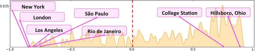
While limited to one type of social media spread and with      for geo-targeted advertising. This work can also comple-
an inherent sample bias towards using who are willing to          ment efforts to model network structures that support (or
share their precise location, the investigation of these ques-    impede) the “viralness” of social media, measure the conta-
tions can provide new insights toward understanding the           gion factors that impact how users influence their neighbors,
spatio-temporal dynamics of the sharing of user-generated         develop models of future social media adoption, and so forth.
content. Our investigation is structured in three steps. First,
we study the global footprint of hashtags and explore the         2. RELATED WORK
spatial constraints on hashtag adoption. In particular, we
analyze the worldwide distribution of hashtags and the im-          Our work presented here builds on two lines of research:
pact distance has on where and when hashtags will be adopted.     studies of Twitter and of Twitter hashtags; and geo-spatial
Second, we study three spatial properties of hashtag propa-       analysis of social media.
gation – focus, entropy, and spread – and examine the spatial     Twitter Hashtag Analysis: There have been several pa-
propagation of hashtags using these properties. Specifically,     pers studying the general properties of Twitter as a social
we study the nature (local or global) of hashtag propagation      network and in analyzing information diffusion over this net-
and the correlation between the spatial properties and the        work [13, 15, 23, 16]. Continuing in this direction most
number of occurrences of the hashtags. Finally, we present        papers related to hashtags have focused their attention on
two methods for characterizing locations based on hashtag         understanding the propagation of hashtags on the network.
spatial analytics. The first method uses spatial properties       For example, in [20] the authors studied factors for hashtag
– entropy and focus – to determine the nature of a loca-          diffusion and found that repeated exposure to a hashtag in-
tion from the point of hashtag propagation, while the sec-        creased the chance of it being reposted again, especially if
ond method uses hashtag adoption times to characterize a          the hashtag is contentious. An approach grounded in linguis-
location’s impact to enable hashtag propagation.                  tic principles has studied the properties of hashtag creation,
   Some of our key findings are:                                  use, and dissemination in [8]. In related research, approaches
                                                                  based on linear regression have been used to predict the pop-
   • Hashtags are a global phenomenon, with locations all
                                                                  ularity of hashtags in a given time frame [22]. Because of
     across the world. But the physical distance between lo-
                                                                  the variety of ways in which hashtags’s are used to convey
     cations is a strong constraint on the adoption of hash-
                                                                  information about a tweet, there has been recent research
     tags, both in terms of the hashtags shared between
                                                                  in hashtag-based sentiment detection [10], topic tracking on
     locations and in the timing of when these hashtags are
                                                                  twitter streams [18], and so forth.
     adopted.
                                                                  Geo-spatial Analysis of Social Media: The emergence
   • Hashtags are essentially a local phenomenon with long-
                                                                  of location-based social networks like Foursquare, Gowalla,
     tailed life spans, but follow a “spray-and-diffuse” pat-
                                                                  and Google Latitude has motivated large-scale geo-spatial
     tern, similar to Youtube videos [5], where initially a
                                                                  analysis [14, 21, 19, 7]. Some of the earliest research related
     small number of locations “champion” a hashtag, make
                                                                  to geo-spatial analysis of web content were based on min-
     it popular, and the spread it to other locations. Af-
                                                                  ing geography specific content for search engines [11]. More
     ter this initial spread, hashtag popularity drops and
                                                                  recently in [2] the authors analyzed search queries to under-
     only locations that championed it originally continue
                                                                  stand the spatial distribution of queries and understand their
     to post it.
                                                                  geographical centers. On Twitter, geo-spatial analysis has
   • The rate at which a hashtag becomes popular is depen-        focused on inferring geographic information from tweets like
     dent on the hashtag’s origin. That is, hashtags that         predicting user locations from tweets [6] and spatial mod-
     originate as responses to external stimuli (like real-       eling to geolocate objects [9]. Similar analysis to infer a
     world events) spread faster than hashtags that origi-        user’s location on Facebook based on their social network
     nate purely within the Twitter network itself (e.g., cor-    has been studied in [3]. Researchers have also analyzed
     responding to a Twitter meme like #ifyouknowmey-             Youtube videos for geo-spatial properties and observed the
     ouknow).                                                     highly-local nature of video views [5].

   • Through hashtag spatial analytics, the relative impact
     of locations can be measured; for example while both
                                                                  3. DATA AND SETUP
     London and Sao Paulo are home to the most total                 We collected a sample of 2 billion geo-tagged tweets con-
     hashtags, hashtags originating in London have a global       taining 342 million hashtags (27 million unique hashtags)
     footprint, while Sao Paulo’s are mostly constrained          from Twitter using the Twitter Streaming API from Febru-
     to Brazil due to inherent language and culture con-          ary 1, 2011 to October 31, 2012. Each tweet in this sample is
     straints.                                                    tagged with a latitude and longitude indicating the location
                                                                  of the user at the time of the posting, resulting in a tu-
   These results can positively impact both research into the     ple of the form < hashtag, time, latitude, longitude >.
spread of online memes as well as systems operators, e.g., in-    The expected long tail distribution for hashtag occurrences
forming the design of distributed content delivery networks       is shown in Figure 1(a).
and search infrastructure for real-time Twitter-like content.        To support location-based analysis, we divide the globe
For example, caching decisions to improve fast delivery of so-    into square grids of equal area using Universal Transverse
cial media content to users and to support applications like      Mercator (UTM), a geographic coordinate system which uses
real-time search can build upon the results presented here.       a 2-dimensional Cartesian coordinate system to map loca-
Insights into the role distance plays and the impact loca-        tions on the surface of the globe [1]. The issue with using
tions have on hashtag spread could inform new algorithms          an angular co-ordinate system like latitudes and longitudes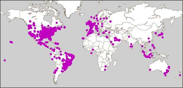
(a) Hashtag distribution      (b) Location distribution

        Figure 1: Hashtag dataset properties
                                                                  Figure 2: Fraction of hashtag occurrences in loca-
                                                                  tions ordered by their rank. The inset plot shows
is that distance covered by a degree of longitude differs as      the fraction for top-200 locations.
we move towards the pole. In addition, the distance covered
by moving a degree in latitude and longitude is same only
at the equator. Hence, it is hard to break globe into grids
using this system. UTM on the other hand gives us a sys-
tem of grids that closely matches distances in metric system
making our analysis easier. While varying the choice of grid
size can allow analysis at multiple levels (e.g., from state-
sized cells to neighborhood-sized ones), we adopt a middle
ground by dividing the globe into squares of 10km by 10km.
Some grid cells will naturally be densely populated, others
will be sparse. Let this set of distinct locations, each cor-
responding to a square, be represented by the set L. With
these locations, we observe in Figure 1(b) that the number of        Figure 3: Top-5 locations with most hashtags
hashtags present in a location follows a long tail distribution
(e.g., 10,000 unique hashtags are observed in 10 locations;
100 unique hashtags are observed in 100 locations), following     4. LOCATION PROPERTIES OF HASHTAGS
the expected population density of equal-sized grid cells.           In this section, we begin our analysis by examining the
   For the rest of the paper, we focus on hashtags with at        locations represented in the dataset and exploring the rela-
least 5 occurrences in a location and with at least 50 total      tionship between locations. In particular, we are interested
occurrences across all locations. Since some hashtags may         in understanding: (i) what is the worldwide distribution of
have begun their Twitter life before the first day of our sam-    hashtags? (ii) does distance between two locations influence
ple while others may have continued on after the last day,        which hashtags they adopt? and (iii) does distance between
we consider both February 2011 and October 2012 as buffer         two locations influence when they will adopt these hashtags?
months. Hence, we capture the full lifecycle of hashtags
starting on or after March 1, 2011 and ending by September        4.1 Location Distribution
30, 2012 which focuses our study to hashtags which have              We first examine the distribution of hashtags across the
both their birth and death within the time of study.              4, 946 unique locations represented in the dataset, as shown
   The rest of this paper considers a set of hashtags H (con-     in Figure 2. The distribution of hashtags occurring in loca-
sisting of close to 20 million hashtags from 99,015 unique        tions ordered by their rank (in terms of number of occur-
hashtags) and a set of locations L (consisting of 4,946 loca-     rences) decreases exponentially with increasing rank, mean-
tions). For every hashtag (h ∈ H) and location (l ∈ L) pair,      ing that the distribution of hashtags in various locations is
we denote the set of all occurrences of h in l as Olh . We say    very uneven. But, focusing on just the top-200 locations (as
that Hl is the set of unique hashtags observed in l.              shown in the inset plot in Figure 2), we see that though the
   Our study continues in three major parts:                      decrease in occurrence is exponential, it is small compared
                                                                  to the drop that we see for all locations in the larger figure,
   • First, we study the global footprint of hashtags and         indicating the presence of locations which generate high but
     explore the spatial constraints on hashtag adoption.         relatively the same number of hashtags.
     (§ 4)                                                           The top-5 locations by their rank are shown in Figure 3.
                                                                  While Sao Paulo claims close to 3.4% of all hashtags and
   • Second, we study three spatial properties of hashtag         no US city occurs in the top-3 positions, when aggregating
     propagation – focus, entropy, and spread – and ex-           locations by country we observe that the US has close to a
     amine the spatial propagation of hashtags using these        40% share followed by Brazil with 6% and the UK with 5%.
     properties. (§ 5)                                               Although the US dominates, if we extend to the top-200
                                                                  most prevalent locations, we see in Figure 4 the global foot-
   • Finally, we illustrate two potential methods for char-       print of hashtags covering most of the major densely popu-
     acterizing locations based on hashtag spatial analytics.     lated cities in the world (sans China).
     (§ 6)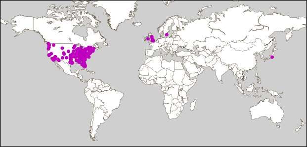
Figure 4: Top-200 locations with the most hashtags.                Figure 5: Hashtag sharing similarity vs Distance.

4.2 Relationship between Locations
   Given the global nature of hashtags, we next examine the
relationship between locations in terms of hashtag adoption.
We consider two approaches that consider the distance be-
tween location pairs – one based on the fraction of hash-
tags shared between locations; the other based on the adop-
tion time lag between locations. In both cases we measure
the distance between locations using the Haversine distance
function, which accounts for the effects of the Earth’s spher-
ical shape in finding distances between points.1 In essence,
the Haversine maps from latitude-longitude pairs to dis-
tance: D : R2 × R2 → R.
                                                                      Figure 6: Hashtag adoption lag vs Distance
Hashtag Sharing vs Distance: We first seek to under-
stand the relationship of the distance between locations on
the commonality of hashtags adopted in locations. To what         the hashtag adoption lag of two locations as:
degree does distance impact whether a hashtag is shared be-
tween two locations? Given two locations, we measure their                                           1            X
                                                                     Adoption Lag(li , lj ) =                               |thli − thlj |
hashtag “similarity” using the Jaccard coefficient between                                      |Hli ∩ Hlj |
                                                                                                               h∈Hl ∩Hl
the sets of hashtags observed at each location:                                                                    i    j

                                            H li ∩ H lj           where the adoption lag measures the mean temporal lag be-
           Hashtag Similarity(li , lj ) =                         tween two locations for hashtags that occur in both the loca-
                                            H li ∪ H lj
                                                                  tions. A lower value indicates that common hashtags reach
where recall Hl is the set of unique hashtags observed in l.      both the locations around the same time. We see in Figure 6
Locations that have all hashtags in common have a similarity      a relatively flat relationship up to ∼500 miles, then a gener-
score of 1.0, while those that share no hashtags have a score     ally positive correlation, suggesting that locations that are
of 0.0. The relationship between hashtag similarity and dis-      close in spatial distance tend also to be close in time (e.g.,
tance is plotted in Figure 5. We see a strong correlation, sug-   they adopt hashtags at approximately the same time). Loca-
gesting that the closer two locations are, the more likely they   tions that are more spatially distant tend to adopt hashtags
are to adopt the same hashtags. As distance increases, the        at greater lags with respect to each other.
hashtag sharing similarity drops accordingly. Much of this
distance-based correlation can be explained by issues of lan-     4.3 Summary
guage, culture and other common interests shared between            Our observations in this section indicate that hashtags
these locations. For example, we see strong similarities in       are fundamentally a global phenomenon, with locations all
hashtags between English-speaking parts of Western Europe         across the world participating in the sharing of this type
and the United States; and between Portuguese-speaking            of social media. However, we have also confirmed that the
parts of Brazil and Portugal.                                     physical distance between locations is a strong constraint
Hashtag Adoption Lag vs Distance: While locations                 on the adoption of hashtags, both in terms of the hashtags
that are near are more likely to share hashtags, are they         shared between locations and in the timing of when these
also more likely to adopt hashtags at the same time? We           hashtags are adopted.
next measure the impact of distance on hashtag adoption
lag between two locations. Locations that adopt a common          5. HASHTAG PROPAGATION
hashtag at the same time can be considered as more tem-
                                                                     Based on the observations in the previous section, we now
porally similar than are two locations that are farther apart
                                                                  focus on the characteristics of hashtag propagations across
in time (with a greater lag). Letting thl be the first time
                                                                  the globe. We examine the spatio-temporal properties of
when hashtag h was observed in location l, we can define
                                                                  individual hashtags to explore questions like: To what de-
1
 For a fuller treatment, we refer the interested reader      to   gree are hashtags a local phenomenon? Does the number
http://en.wikipedia.org/wiki/Haversine formula                    of occurrences of hashtag impact its global spread? Can we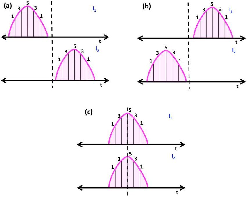
characterize the spatial properties of local and global hash-
tags?
5.1 Spatial Properties of Hashtag Propagation
   Previous studies of the geographic scope of social media
and web resources have typically adopted two types of mea-
sures: one considering the intensity of focus and one con-
sidering the uniformity of this interest. Similarly, we adopt
two measures (similar to ones for studying YouTube videos                    (a) CDF               (b) Mean hashtag focus
in [5]): hashtag focus and hashtag entropy, plus a third mea-
sure called the hashtag spread.                                   Figure 7: Focus: Around 50% of hashtags accumu-
   For every hashtag (h ∈ H) and location (l ∈ L) pair, if        late at least 50% of their postings from a single lo-
we let Olh be the set of all occurrences of h in l, then the      cation.
probability of observing hashtag h in location l is defined as:
                                     Olh
                       Plh = P           h
                                   l∈L {Ol }

     Then the hashtag focus for hashtag h is:
                         F h = max Plh
                                  l∈L

which is simply the maximum probability of observing the
hashtag at a single location. The location at which the prob-                (a) CDF             (b) Mean hashtag entropies
ability is maximum is called the hashtag focus location. As
a hashtag propagates, intuitively its focus will reduce as the
hashtag is observed at multiple locations. The more local a       Figure 8: Entropy: Almost 20% of hashtags are
hashtag is, presumably the higher its focus will be as well.      confined to a single location, but hashtags begin to
Note that we additionally denote the focus measured over          spread as they become popular.
an interval t (rather than over the entire dataset) as F h (t).
  The hashtag entropy is defined as:
                                                                  5.2 Local versus Global: Measuring Focus, En-
                                                                      tropy, and Spread
                            X h
                    Eh = −     Pl log2 Plh
                             l∈L                                    Using these three spatial properties, we now analyze the
which measures the randomness in spatial distribution of          properties of hashtag propagations.
a hashtag and determines the minimum number of bits re-           Measuring Hashtag Focus: We begin by considering the
quired to represent the spread. A hashtag that occurs in          focus values of hashtags. The cumulative distribution for fo-
only a single location will have an entropy of 0.0. As a          cus values of hashtags is shown in Figure 7(a). We observe
hashtag spreads to more locations, its entropy will increase,     that the distribution is nearly linear, meaning that the fo-
reflecting the greater randomness in the distribution. Like       cus values for hashtags are uniformly distributed. We also
focus, we can additionally denote the entropy measured over       notice that most hashtags are concentrated in one location.
an interval t (rather than over the entire dataset) as E h (t).   Specifically, around 50% of hashtags derive at least 50% of
   While focus and entropy provide insights into a hashtag’s      their postings from a single location. In addition, as indi-
locality, they lack explicit consideration for the distance a     cated by the single dot at CDF = 1.0, about a quarter of
hashtag has traveled. For example, consider two hashtags –        all hashtags are observed in a single location only. Continu-
one distributed equally between Austin and Dallas, and an-        ing this look at hashtag focus, we next plot the relationship
other one equally distributed between Los Angeles and New         between the number of occurrences of a hashtag and its fo-
York. The focus of both hashtags is 0.5 and their entropy is      cus in Figure 7(b). As can be expected, we observe that
1. Hence, to measure the greater “dispersion” of the LA-NY        hashtags with a few occurrences have a high focus (meaning
hashtag, we define the hashtag spread of hashtag h as:            that these low-intensity hashtags tend to occur primarily in
                         1 X                                      a single location), whereas an increasing number of occur-
                 Sh =             D(o, G(Oh ))
                       |Oh |                                      rences corresponds to a decrease in the focus of the hash-
                             o∈Oh
                                                                  tag. Together, these results suggest that many hashtags
which measures the mean distance for all occurrences of a         correspond to either local events (e.g., #momentoschampi-
hashtag from its geographic midpoint. Here, G is the ge-          ons, #nyadaauditions) or geographically compact networks
ographic midpoint2 for a set of occurrences, which is sim-        of friends. But as hashtags become more popular they tend
ilar to calculating the midpoint on a plane for a set of 2-       to spread to more locations. That is, it is unlikely for a
dimensional points, but as in the case of Haversine distance,     popular hashtag to be constrained to a handful of locations;
the geographic midpoint is calculated by considering the ef-      there is spillover from one location to the next.
fects of Earth’s spherical shape. A local hashtag with many
                                                                  Measuring Hashtag Entropy: To further explore this
occurrences close to its midpoint will yield a small spread,
                                                                  spatial distribution, we next consider the entropy of hash-
while a global hashtag with occurrences relatively far from
                                                                  tag propagations. Recall that an entropy of zero for a hash-
its center will yield a larger spread.
                                                                  tag indicates that it was posted from one (20 ) location only,
2
    http://www.geomidpoint.com/                                   while, for example, an entropy value of two indicates a hash-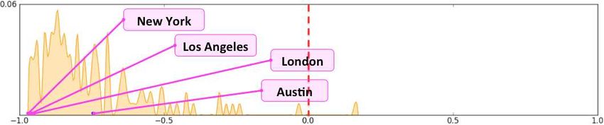
(a) CDF                (b) Mean hashtag spread

Figure 9: Spread: 50% of hashtags have a spread
less than 400 miles; 25% of hashtags have a spread
greater than 1000 miles.                                                     Figure 10: Entropy versus Focus.

tag propagated almost equally to four (22 ) locations. The
cumulative distribution of entropy in Figure 8(a) shows that
about 25% of hashtags are concentrated in a single location
and that the majority of hashtags propagate to at most two
locations. On the flipside, however, we do see that hashtags
with many occurrences tend to spread to many locations, as
seen by the increasing entropy versus the number of hashtag            (a) Focus vs Spread.          (b) Entropy vs Spread.
occurrences in Figure 8(b) (and the decreasing focus values,
as we observed in Figure 7(b)). As a hashtag becomes pop-
ular it tends to spread to newer locations and this in turn        Figure 11: Correlation between spatial properties
makes it more popular. These results show that the major-          and spread.
ity of hashtags have a narrow base of geographic support,
but that one of the keys to popularity is a broad geographic
                                                                   decreasing focus until 4000 miles. The initial steep drop of
footprint. This is intuitively sensible, but important to con-
                                                                   focus indicates that the locations that are adopting hash-
firm in practice.
                                                                   tags are spatially close to each other. On a map, the spatial
Measuring Hashtag Spread: While focus and entropy                  distribution of these hashtags would look like a tight cluster
provide insights into a hashtag’s locality, neither directly       of dots in a small region. The next region where the focus
measures the geographic area over which a hashtag prop-            remains almost the same while the spread increases corre-
agates. Using hashtag spread, we see in Figure 9(a) that           sponds to hashtags that are spatially well distributed but
about a quarter of hashtags have a spread of zero since they       the majority of hashtags are being produced by a single lo-
were observed in only location. In addition, we observe that       cation. On a map the spatial distribution for these hashtags
most hashtags have a small spread, with almost 50% of hash-        would have dots spread over a wide region as in Figure 12(a),
tags having a spread less than 400 miles. However, we do           but with only a few of those dots generating the majority of
observe that around 25% of hashtags have a spread greater          hashtags. Finally, the third region corresponds to globally
than 1000 miles. We next plot the correlation between num-         distributed hashtags like the one shown in Figure 12(b). We
ber of occurrences of a hashtag and its spread in Figure 9(b).     see similar behavior when we plot entropy against spread as
Consistent with the findings over focus and entropy we ob-         shown in Figure 11(b): a steep increase in entropy for the
serve that an increasing number of occurrences is coupled          first 700 miles, then a region until about 1600 miles with
with a larger spatial footprint.                                   uniform entropy and finally a region of increasing entropy
                                                                   until 4000 miles.
Direct Comparison of Spatial Properties: We now                       In summary, most hashtags are essentially a local phe-
turn to directly comparing the focus, entropy, and spread          nomenon, as indicated by the on-average high focus, low
values for our hashtags. We begin by plotting the mean             entropy, and small spread. But as a hashtag becomes more
hashtag focus on the x-axis versus the mean hashtag en-            popular, we see a decrease in focus and an increase in en-
tropy on the y-axis, as shown in Figure 10. Local hashtags         tropy and spread, all hallmarks of global impact. Based on
– with a high focus and a low entropy – are located in the         the analysis in this section, we identify three broad cate-
bottom-right of the figure; global hashtags – with a low fo-       gories of hashtags:
cus and a high entropy – are located in the top-left of the
figure.                                                               • Local Interest [60% of all hashtags]: These hash-
   The correlation between spread and our two other spatial             tags have a spread range from 0 to 700 miles. They
properties – focus and entropy – is shown in Figure 11. As              have a high focus with median of 0.79 and low en-
expected, an increasing spread results in a decreasing focus            tropy of 1 bit. Example local interest hashtags include
because as a hashtag spreads it occurs in more locations                #volunteer4betterindia, #ramadanmovies, and #once-
which in turn reduces the overall focus. For similar reasons            uponatimeinnigeria.
we observe an increase in entropy with increasing spread.
   We also observe that in Figure 11(a), there is a steep drop        • Regional and Event-Driven [15% of all hash-
in focus for the first 700 miles, followed by a region of almost        tags]: These hashtags have a spread range from 700
uniform focus until about 1600 miles and finally a region of            to 1000 miles. They have a median focus of 0.44 and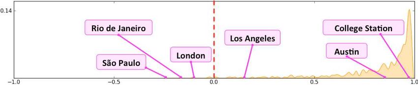
(a) #cnndebate                (b) #ripstevejobs

       Figure 12: Example of hashtag spread.

                                                                      Figure 14: CDF of occurrences with time.

(a) Distribution of hashtag (b) CDF for hashtag peaks.
peaks.
                                                                 (a) Hashtags that peak dur- (b) Hashtags that peak be-
          Figure 13: Hashtag peak analysis.                      ing the first 30 minutes.   tween 4 and 10 hours

                                                                 Figure 15: (Color) Comparing the spatial properties
     entropy of 3 bits. Example regional and event-driven
                                                                 of hashtags that reach their peak quickly (a) and
     hashtags include#cnbcdebate, #iowadebate, etc.
                                                                 those that reach their peak more slowly (b). Local
   • Worldwide Phenomena [25% of all hashtags]:                  hashtags – with a high focus and a low entropy – are
     These hashtags have a spread range from 1000 to 4000        located in the bottom-right of each figure; global
     miles. These are mostly global hashtags which have          hashtags – with a low focus and a high entropy –
     low focus with median of 0.28 and entropy of 4 bits.        are located in the top-left of each figure. Low peak
     Example worldwide phenomena hashtags include #brit-         values are in light blue; high peak values in magenta.
     neyvmas, #yearof4, #timessquareball.

5.3 Slow versus Fast: Peak Analysis                              slower hashtags, shown in Figure 15(b), where the global
   We next augment our analysis by considering, in addi-         hashtags are relatively faster than the local hashtags. On
tion to the spatial propagation of hashtags, the temporal        closer inspection, we attribute this reversal to the motive
characteristics of these hashtags. We begin this temporal        or purpose of the hashtags. First, we observe that hash-
analysis by studying when hashtags reach the peak of their       tags that peak slowly are mostly of anticipated events, like
propagation in terms of occurrences. For this study we fo-       the hashtag “#mtvema” corresponding to the MTV music
cus on hashtags that reach their peak within the first two       awards, while the hashtags that peak more quickly are those
days after their first appearance. We see in Figure 13(a) the    that are organically generated within Twitter and related to
distribution of peak times across all hashtags. We find that     fun like “#childhoodmemories”. Second, slower hashtags are
around 20% of hashtags reach their peak within 20 minutes        not as dependent on social sharing within Twitter as com-
of their first appearance. The distribution of peaks falls ex-   pared to faster hashtags; for example, users may be aware
ponentially after that. We also observe that about 60% of all    about the MTV awards from multiple sources (TV, news,
hashtags reach their peak within the first 2 hours as shown in   friends), while the hashtag “#childhoodmemories” is seen
Figure 13(b). In addition we observe that on average hash-       only by those on Twitter. This dependency on the network
tags accumulate more than 50% of their total occurrences in      to spread makes local fast hashtags peak sooner than the
the first 2 hours of their propagation as shown in Figure 14.    global fast hashtags. The global slow hashtags peak sooner
   But what are the differences between fast-peaking hash-       than the local slow hashtags since more people are aware
tags and slow-peaking ones? Do hashtags behave differently       about them and they are not dependent on the network.
in terms of their spatial properties? To answer these ques-         Based on this peak analysis, we group hashtags into three
tions, we consider two sets of hashtags – those that reach       categories:
their peak within the first 30 minutes of their initial ap-
pearance and a second set consisting of slower hashtags that        • Fast [25% of all hashtags]: These hashtags reach
reach their peak between 4 and 10 hours of their initial ap-          their peak within 30 minutes of their first appearance.
pearance. To analyze the relationship between locality and            We find that 65% of these hashtags are local, 15% of
peak times we plotted these sets of hashtags in Figure 15,            these hashtags are national or event driven and 20%
with focus on the x-axis and entropy on the y-axis.                   are global.
   We observe that in the set of faster hashtags – which
reach a peak within 30 minutes of their propagation – the           • Medium [20% of all hashtags]: These hashtags
local hashtags are much faster than the global ones (see              reach their peak between 30 minutes and 10 hours af-
Figure 15(a)). This observation is reversed in the set of             ter their first appearance. We find that 55% of these
occurrences from a single location. With this in mind, we
find that hashtags receive most of their occurrences from
this single location during their peak explaining the spike
in interval focus and the fall in interval entropy. In effect,
this single location is “championing” a hashtag. In the 10-20
minutes after this peak period, other locations adopt the
hashtag, resulting in a decrease in interval focus and an
(a) Interval focus with time. (b) Interval entropy with increase in entropy as the hashtags becomes more global.
time. About 30 minutes after reaching peak, focus and entropy
reverse, with focus increasing and entropy decreasing as the
Figure 16: Hashtags peak with their most “global” hashtag withdraws back to its original focus location.
footprint 10-20 minutes after their peak In essence, hashtags are spread via a single location “cham-
pioning” a hashtag initially, spreading it to other locations
and then continuing to propagate it after it has become
hashtags are local, 17% of these hashtags are national popular. In [5], the authors observed a similar pattern for
or event driven and 28% are global. YouTube videos which they called the “spray-and-diffuse”
pattern. Our observations over hashtags suggest that this
• Slow [55% of all hashtags]: These hashtags reach
pattern may be a fundamental property of social media spread.
their peak more than 10 hours after their first appear-
ance. We find that 60% of these hashtags are local,
16% of these hashtags are national or event driven and 6. HASHTAG-BASED SPATIAL ANALYTICS
24% are global.
Finally, we turn our sights towards leveraging the spatio-
For all three peak-based categories we observe that the temporal propagation of hashtags to characterize locations.
distribution of spatial categories is quite similar. Are some locations more “impactful” in terms of the hashtags
that originate there, and other locations more “impression-
5.4 Patterns of Hashtag Propagation able” in terms of hashtags they propagate? Concretely, we il-
We next zoom in on the spatial properties of hashtag prop- lustrate two techniques for characterizing locations based on
agation during the minutes pre- and post- peak. When hash- hashtag spatial analytics: (i) location-based entropy-focus-
tags peak, do they peak suddenly in different locations si- spread plots; and (ii) a method for evaluating the spatial
multaneously or do they slowly accumulate a larger spatial impact of locations.
footprint? What are the dynamics of their spatial properties
as they become popular? 6.1 Entropy-Focus-Spread Plots
For this study, we divide each hashtag’s lifecycle into equal In the first technique, we first assign every hashtag to its
length time intervals of 10 minutes. For each time interval, corresponding hashtag focus location. This results in every
we compute the hashtag focus (F h (t)) and the hashtag en- location having a set of hashtags that were focused there.
tropy (E h (t)) over just that interval. We plot these interval- Using this set of hashtags we plot the entropy versus focus
specific focus and entropy measures in Figure 16. First, for every hashtag focused on this location plus indicate the
compared to the aggregate characteristics across all hash- mean spread for every focus-entropy pair using a color gradi-
tags – in which we find the median focus for all hashtags ent. To illustrate, consider the four location-based entropy-
over their entire lifetime to be 0.57; for entropy, we find a focus-spread plots in Figure 17 – one for London, Sao Paulo,
median of 2 bits – here we see that the interval-based fo- Ankara, and Los Angeles. Recall that London, Sao Paulo,
cus is even higher (greater than 0.80 in all cases) and the and Los Angeles are among the top-5 locations in terms of
interval-based entropy is even lower (less than 1 bit in all total hashtags, while Ankara ranks much lower.
cases). These higher focus / lower entropy results indicate First, we observe that locations that have high hashtag
that hashtags are even more local during each step of their counts have a complete spectrum of hashtags on the plots.
propagation. To illustrate, in the aggregate we may find a Recall that local hashtags occur on the right-bottom of such
hashtag that propagates only in locations in Texas. Com- plots, while global hashtags are on the left-top. Here we see
pared to a global hashtag, it is certainly more local and that the popular locations are the focal points (or “cham-
its focus and entropy will reflect this. However, during its pions”) for both local and global hashtags. Ankara, on the
propagation, the Texas-based hashtag is even more local at other hand, is the focal point for only relatively local hash-
each step; that is, it does not propagate over the entire state tags (with high focus and low entropy).
simultaneously but in stages, city by city. It might first be- Second, the use of spread (with high values in a lighter
come popular in Dallas, then in Austin, and so on. yellow, while lower values of spread are in red) illustrates
Returning to Figure 16(a) and Figure 16(b), we observe the relative geo-spatial footprint of hashtags that have a lo-
that hashtags reach their lowest interval focus and high- cation as its focal point. For example, although Sao Paulo
est interval entropy about 10-20 minutes after their peak. has a high total number of hashtags and a high number of
Rather than peaking with their most “global” footprint, hash- total locations impacted (note the hashtags with low focus
tags instead reach this state after their peak. This result – and high entropy), the geospatial footprint of Sao Paulo is
that a peaking hashtag is actually more local than it ul- relatively low (note the very little yellow among these hash-
timately will be – is seemingly counterintuitive. However, tags). The hashtags popular in Sao Paulo have high entropy
recall that in our in our examination of the cumulative dis- because they are spread over several locations but all these
tribution of focus shown in Figure 7(a), we noted that al- locations are close to each other resulting in a smaller spread.
most 50% of hashtags accumulate more than 50% of their Los Angeles on the other hand has a global impact; hashtags(a) London (b) Sao Paulo
(c) Ankara (d) Los Angeles
Figure 17: (Color) Entropy-Focus-Spread plots for
four cities. Local hashtags – with a high focus and
Figure 18: Example of hashtag adoption for two lo-
a low entropy – are located in the bottom-right of
cations l1 and l2 . In (a) l1 adopts all of its hashtags
each figure; global hashtags – with a low focus and
before l2 . In (b) l1 adopts all of its hashtags after l2 .
a high entropy – are located in the top-left of each
In (c) l1 and l2 adopt hashtags simultaneously.
figure. The mean spread for every focus-entropy
pair using a color gradient: high values in a lighter
yellow, while lower values of spread are in red.
where, Ilhi →lj is defined as:
|Olh ≺Olh |−|Olh ≻Olh |
i j i j
if h ∈ Hli and h ∈ Hlj
that become popular in Los Angeles tend to be popular in
|Olh ×Olh |
h
a larger geographical area. Ili →lj = i j
1 if h ∈ Hli only
−1 if h ∈ Hlj only
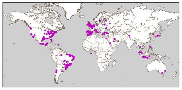
6.2 Measuring Spatial Impact
The second spatial analytics technique directly evaluates The impact is 1 if a hashtag is posted only in li , as li clearly
the impact a location has on other locations by measuring impacts lj in this case. For similar reasons the impact is −1
the hashtag-based spatial impact. We define the spatial im- when a hashtag is posted only in lj . To understand the case
pact Ili →lj of location li on lj as a score in the range [−1, 1], when a hashtag is observed in both the locations consider the
such that −1 indicates li adopts a hashtag only after lj has example shown in Figure 18. In all three cases |Olh1 | = 13,
adopted it, +1 indicates lj adopts a hashtag only after li |Olh2 | = 13 and |Olh1 × Olh2 | = 169.
adopts it and 0 indicates the locations are independent of • Case (a): |Olh1 ≺ Olh2 | = 169 and |Olh1 ≻ Olh2 | = 0.
each other and adopt hashtags simultaneously. Hence, Ilhi →lj = 169−0 = 1.
169
For example, consider the three cases shown in Figure 18.
When hashtags are generated between a pair of locations • Case (b): |Olh1 ≺ Olh2 | = 0 and |Olh1 ≻ Olh2 | = 169.
as shown in (a) we want Il1 →l2 = 1, when as shown in (b) Hence, Ilhi →lj = 0−169
169
= −1.
we want Il1 →l2 = −1, and when as shown in (c) we want
• Case (c): |Olh1 ≺ Olh2 | = 62 and |Olh1 ≻ Olh2 | = 62.
Il1 →l2 = 0. Let ohl (t) represent an occurrence of hashtag h
in location l at time interval t. Then, we define the preceding Hence, Ilhi →lj = 62−62
169
= 0.
operator ≺ over two sets of occurrences Olhi and Olhj as: We visualize the spatial impact of a location using a spa-
tial impact plot. The x-axis represents the spatial impact
Olhi ≺ Olhj = {ohli (t) | ti < tj ∀ (ohli (t1 ), ohlj (t2 )) ∈ Olhi × Olhj } values and is in the range [−1, 1]; the y-axis shows the dis-
tribution of locations at these values. Examples of impact
which gives a set of all occurrences of h in l1 that precede l2 plots for three locations can be found in Figure 19. In every
in the cartesian product of their occurrences. Similarly, we impact plot, locations on the left half of the plot are impact-
define the succeeding operator ≻ as: ing locations and the locations on the right half of the plot
are impacted locations. Hence, plots for famous and large
Olhi ≻ Olhj = {ohli (t) | ti > tj ∀ (ohl1 (t1 ), ohlj (t2 )) ∈ Olhi × Olhj } locations are generally right-heavy as they impact many lo-
cations. Plots for small locations are mostly left-heavy as
which gives the set of all occurrences of h in l1 that succeed they are impacted by many locations. For example, the im-
l2 in the cartesian product of their occurrences. We now pact plot for New York is right heavy since New York is an
define the spatial impact of location li on lj as the aver- “early adopter” with a high spatial impact on other loca-
age of hashtag specific spatial impact values, Ilhi →lj , for all tions. Interestingly, New York is actually impacted by both
hashtags that occur in both the locations: Sao Paulo and Rio de Janeiro, since Portuguese hashtags
tend to flow from Brazil to Portuguese-speaking neighbor-
Ilhi →lj hoods in New York, whereas hashtags from New York are
P
h∈Hl ∪Hl
i j
Ili →lj = less likely to flow to Brazil. College Station (home to Texas
|Hli ∪ Hlj | A&M) is fairly small, with a left-heavy distribution, indicat-(a) New York
(b) Austin
(c) College Station
Figure 19: Spatial impact plots for three locations. Locations to the left of the origin are “early adopters”
relative to the baseline location. New York has a high impact, with almost all cities to the right of its origin.
College Station, on the other hand, is low impact since it only adopts hashtags after almost all other cities.
ing that it is a “late adopter”. Austin, on the other hand, representing a globally known event reaches its peak much
has a balanced spatial impact, being both impacted by many faster than either locally-known events or hashtags spread
locations and impacting many other locations. purely within the network (e.g., #ifyouknowmeyouknow).
Based on spatial and temporal categories we classified hash-
tags into different categories. In our continuing work we are
7. CONCLUSION interested in hashtag category specific analysis. We want
In this paper, we have analyzed the spatio-temporal dy- to study how the temporal characteristics of hashtags may
namics of social media propagation through a study of 2 differ depending upon their spatial categories.
billion geo-tagged Tweets. Our study has consisted of three
key parts: (i) a study of the global footprint of hashtags and 8. ACKNOWLEDGMENTS
an exploration of the spatial constraints on hashtag adop-
This work was supported in part by NSF grant IIS-1149383
tion; (ii) a study of three spatial properties of hashtag prop- and a Google Research Award. Any opinions, findings and
agation – focus, entropy, and spread – and an examination conclusions or recommendations expressed in this material
of the spatial propagation of hashtags using these proper-
are the author(s) and do not necessarily reflect those of the
ties; and (iii) two spatial analytics techniques for character-
sponsors.
izing the relative impact of locations. We have found that
hashtags are a global phenomenon, with locations all across
the world. But the physical distance between locations is a 9. REFERENCES
strong constraint on the adoption of hashtags, both in terms [1] Universal transverse mercator coordinate system,
of the hashtags shared between locations and in the timing November 2012.
of when these hashtags are adopted. We have also found [2] L. Backstrom, J. Kleinberg, R. Kumar, and J. Novak.
that hashtags are mostly a local phenomenon with long- Spatial variation in search engine queries. In
tailed life spans, but follow a “spray-and-diffuse” pattern [5] Proceeding of the 17th international conference on
where initially a small number of locations “champion” a World Wide Web, pages 357–366. ACM, 2008.
hashtag, make it popular, and the spread it to other loca- [3] L. Backstrom, E. Sun, and C. Marlow. Find me if you
tions. We have found both spatial and temporal locality as can: improving geographical prediction with social
most hashtags spread over small geographical areas but at and spatial proximity. In Proceedings of the 19th
high speeds. The purpose of a hashtag and its global aware- international conference on World wide web, pages
ness determines how fast it will reach its peak. A hashtag 61–70. ACM, 2010.[4] C. Bauckhage. Insights into internet memes. Proc. [15] H. Kwak, C. Lee, H. Park, and S. Moon. What is
ICWSM2011, pages 42–49, 2011. twitter, a social network or a news media? In
[5] A. Brodersen, S. Scellato, and M. Wattenhofer. Proceedings of the 19th international conference on
Youtube around the world: geographic popularity of World wide web, pages 591–600. ACM, 2010.
videos. In Proceedings of the 21st international [16] K. Lerman and R. Ghosh. Information contagion: An
conference on World Wide Web, pages 241–250. ACM, empirical study of the spread of news on digg and
2012. twitter social networks. In Proceedings of 4th
[6] Z. Cheng, J. Caverlee, and K. Lee. You are where you International Conference on Weblogs and Social Media
tweet: a content-based approach to geo-locating (ICWSM), 2010.
twitter users. In Proceedings of the 19th ACM [17] J. Leskovec, L. Backstrom, and J. Kleinberg.
international conference on Information and Meme-tracking and the dynamics of the news cycle. In
knowledge management, pages 759–768. ACM, 2010. Proceedings of the 15th ACM SIGKDD international
[7] Z. Cheng, J. Caverlee, K. Lee, and D. Sui. Exploring conference on Knowledge discovery and data mining,
millions of footprints in location sharing services. pages 497–506. ACM, 2009.
AAAI ICWSM, 2011. [18] J. Lin, R. Snow, and W. Morgan. Smoothing
[8] E. Cunha, G. Magno, G. Comarela, V. Almeida, techniques for adaptive online language models: topic
M. Gonçalves, and F. Benevenuto. Analyzing the tracking in tweet streams. In Proceedings of the 17th
dynamic evolution of hashtags on twitter: a ACM SIGKDD international conference on Knowledge
language-based approach. In Proceedings of the discovery and data mining, pages 422–429. ACM,
Workshop on Language in Social Media (LSM 2011), 2011.
pages 58–65, 2011. [19] A. Noulas, S. Scellato, C. Mascolo, and M. Pontil. An
[9] N. Dalvi, R. Kumar, and B. Pang. Object matching in empirical study of geographic user activity patterns in
tweets with spatial models. In Proceedings of the fifth foursquare. ICWSM’11, 2011.
ACM international conference on Web search and [20] D. Romero, B. Meeder, and J. Kleinberg. Differences
data mining, pages 43–52. ACM, 2012. in the mechanics of information diffusion across topics:
[10] D. Davidov, O. Tsur, and A. Rappoport. Enhanced idioms, political hashtags, and complex contagion on
sentiment learning using twitter hashtags and smileys. twitter. In Proceedings of the 20th international
In Proceedings of the 23rd International Conference on conference on World wide web, pages 695–704. ACM,
Computational Linguistics: Posters, pages 241–249. 2011.
Association for Computational Linguistics, 2010. [21] S. Scellato, A. Noulas, R. Lambiotte, and C. Mascolo.
[11] J. Ding, L. Gravano, and N. Shivakumar. Computing Socio-spatial properties of online location-based social
geographical scopes of web resources. ., 2000. networks. Proceedings of ICWSM, 11:329–336, 2011.
[12] Foursquare. About foursquare, April 2013. [22] O. Tsur and A. Rappoport. What’s in a hashtag?:
[13] B. A. Huberman, D. M. Romero, and F. Wu. Social content based prediction of the spread of ideas in
Networks that Matter: Twitter Under the Microscope. microblogging communities. In Proceedings of the fifth
Social Science Research Network Working Paper ACM international conference on Web search and
Series, Dec. 2008. data mining, pages 643–652. ACM, 2012.
[14] K. Y. Kamath, J. Caverlee, Z. Cheng, and D. Z. Sui. [23] J. Yang and J. Leskovec. Modeling information
Spatial influence vs. community influence: modeling diffusion in implicit networks. In Data Mining
the global spread of social media. In Proceedings of the (ICDM), 2010 IEEE 10th International Conference
21st ACM international conference on Information on, pages 599–608. IEEE, 2010.
and knowledge management, CIKM ’12, pages
962–971, New York, NY, USA, 2012. ACM.You can also read