On the Influence of Optimizers in Deep Learning-based Side-channel Analysis
←
→
Page content transcription
If your browser does not render page correctly, please read the page content below
On the Influence of Optimizers in Deep
         Learning-based Side-channel Analysis

                       Guilherme Perin and Stjepan Picek

                  Delft University of Technology, The Netherlands

      Abstract. The deep learning-based side-channel analysis represents a
      powerful and easy to deploy option for profiled side-channel attacks. A
      detailed tuning phase is often required to reach a good performance
      where one first needs to select relevant hyperparameters and then tune
      them. A common selection for the tuning phase are hyperparameters
      connected with the neural network architecture, while those influencing
      the training process are less explored.
      In this work, we concentrate on the optimizer hyperparameter, and we
      show that this hyperparameter has a significant role in the attack perfor-
      mance. Our results show that common choices of optimizers (Adam and
      RMSprop) indeed work well, but they easily overfit, which means that
      we must use short training phases, small profiled models, and explicit
      regularization. On the other hand, SGD type of optimizers works well
      on average (slower convergence and less overfit), but only if momentum
      is used. Finally, our results show that Adagrad represents a strong option
      to use in scenarios with longer training phases or larger profiled models.

Keywords: Side-channel Analysis · Profiled Attacks · Neural Networks · Opti-
mizers

1   Introduction

Side-channel attacks (SCA) are non-invasive attacks against security-sensitive
implementations [16]. When running on embedded devices, cryptographic im-
plementations need to be protected against such attacks by implementing coun-
termeasures at software and hardware levels. If not sufficiently SCA-resistant,
an adversary can measure side-channel leakages like power consumption [12] or
electromagnetic emanation [25]. Then, the attacker can apply statistical analysis
to recover secrets, including cryptographic keys, and compromise the product.
Side-channel attacks can be mainly divided into unsupervised (or non-profiled)
and supervised (or profiled) attacks. Unsupervised methods include simple anal-
ysis, differential analysis [12], correlation analysis [1], and mutual information
analysis [6]. Supervised attacks are mainly template attacks [3], stochastic at-
tacks [27], and machine learning-based attacks [10,22]. The profiling or training
phase in supervised attacks assumes that the adversary has a device under con-
trol that is identical (or close to identical) to the target device. This way, he can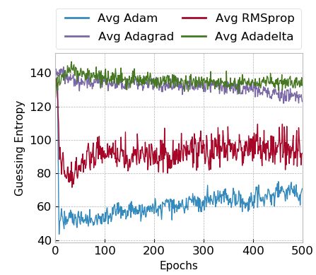
query multiple cryptographic executions with different keys and inputs to cre-
ate a training set and learn a statistical model from side-channel leakages. The
test or attack phase is then applied to a new device identical to the profiling
device. If the profiled model provides satisfactory generalization, the adversary
can recover secrets from the target device.
    Recently, deep learning methods have been applied to side-channel analy-
sis [15,2,11]. The main deep learning algorithms used in profiled SCA are mul-
tilayer perceptron (MLP) and convolutional neural networks (CNNs). The ap-
plication of these techniques opened new perspectives for SCA-based security
evaluations mainly due to the following advantages: 1) CNNs demonstrated to
be more robust against desynchronized side-channel measurements [2], 2) CNNs
and MLPs show the capacity of learning high-order leakages from protected
targets [11], 3) preprocessing phases for feature extraction (points of interest)
are done implicitly by the deep neural network, and 4) techniques like visual-
ization [17,8] can help to identify where a complex learning algorithm detects
leakages from side-channel measurements.
    Despite all the success, the research in the field of deep learning-based SCA
continuously seeks for improvements. There, a common option is to optimize
the behavior of neural networks by tuning their hyperparameters. Some of those
hyperparameters are commonly explored, like the number of layers/neurons and
activation functions [29,24]. Some other hyperparameters receive much less at-
tention. Unfortunately, it is not easy to select all the hyperparameters relevant
to a specific problem or decide how to tune them. Indeed, the selection of opti-
mal hyperparameters for deep neural networks in SCA requires understanding
each of them in the learning phase. The modification of one hyperparameter may
have a strong influence on other hyperparameters, making deep neural networks
extremely difficult to be tuned.
    We can informally divide the hyperparameters into those that influence the
architecture (e.g., number of neurons and layers, activation functions) and those
that influence the training process (e.g., optimizer, loss function, learning rate).
Interestingly, the first category is well-explored in SCA with papers discussing
methodologies or providing extensive experimental results [31,24]. The second
category is much less explored, see, e.g., [13]. One of those less explored (or,
not explored) hyperparameters is the optimizer. With the learning rate, the
optimizer minimizes the loss function and, thus, improves neural networks’ per-
formance. Despite its importance, this hyperparameter is commonly overlooked
in SCA, and researchers usually either do not tune it at all or provide only a
limited set of options to investigate.
   There are several reasons why to explore the influence of optimizers on the
performance of deep learning-based SCA:
 1. As already stated, the optimizer is an important hyperparameter for tuning
    neural networks, but up to now, it did not receive much attention. More
    precisely, the researchers investigated its significance in the context of SCA
    only marginally.

                                         2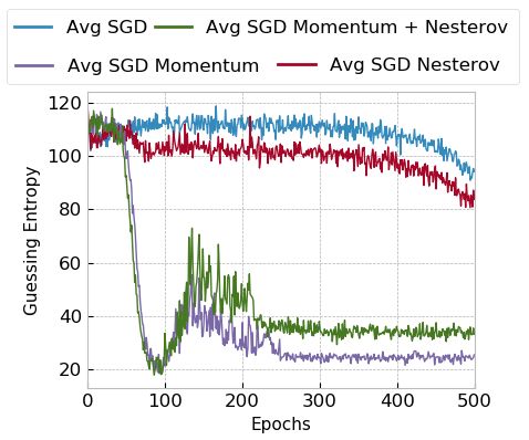
2. Recent works showed that even relatively shallow deep learning architectures
    could reach top performance in SCA [31,11]. This means that we do not have
    issues with the network capacity (i.e., the network’s ability to find a good
    mapping between inputs and outputs and generalize to the new measure-
    ments). This makes the search for a good neural network architecture easier
    as it limits the number of hyperparameter tuning experiments one needs to
    conduct. Simultaneously, we need to be careful to train the neural networks
    well, which means finding good weight parameter values that will not cause
    getting stuck in local optima.
 3. Finally, there is a well-known discrepancy between machine learning and
    side-channel analysis metrics [21]. It is far from trivial to decide when to stop
    the training process to avoid overfitting. Different optimizers show different
    behavior where overfitting does not occur equally easy. Instead of finding
    new ways to indicate when to stop the training [19], we can also explore
    whether there is a more suitable choice of optimizers that are more aligned
    with the SCA goals.
    To provide detailed results, we run experiments on two datasets and numer-
ous scenarios, which resulted in more than 700 hours of continuous GPU runtime.
We analyze two categories of optimizers: stochastic gradient descent (SGD) and
adaptive gradient methods (Adam, RMSprop, Adagrad, and Adadelta). Our re-
sults show that when using SGD optimizers, momentum should always be used.
What is more, with Nesterov, it additionally reduces the chances to overfit. At
the same time, these optimizers require a relatively long training process to con-
verge. While less pronounced, such optimizers can also overfit, especially for long
training phases.
    From adaptive optimizers, Adam and RMSprop work the best if one uses
short training phases. Unfortunately, these optimizers also easily overfit, which
means extra care needs to be taken (for instance, to develop an appropriate
early stopping mechanism). Since those two optimizers overfit for longer training
phases, they also work better for smaller profiled models. Finally, if one requires
longer training phases or larger profiled models, Adagrad behaves the best. We
consider this to be very interesting as Adagrad is not commonly used in profiled
SCA. This finding could be especially relevant in future research when more
complex datasets are considered, and we are forced to use profiled models that
have a larger capacity. Interestingly, in some of our results, we also observe a
deep double descent phenomenon [18], which indicates that longer training is
not always better. This is the first time this phenomenon is observed in the SCA
domain to the best of our knowledge.

2     Background
2.1   Profiled SCA and Deep Learning
We consider a typical profiled side-channel analysis setting. A powerful attacker
has a device (clone device) with knowledge about the secret key implemented.
The attacker can obtain a set of N profiling traces X1 , . . . , XN (where each

                                         3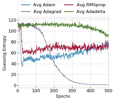
trace corresponds to the processing or plaintext or ciphertext Tp ). With this
information, he calculates a leakage model Y (Tp , k ∗ ). Then, the attacker uses
that information to build a profiling model f (thus, this phase is commonly
known as the profiling phase). The attack is carried out on another device by
using the mapping f . The attacker measures an additional Q traces X1 , . . . , XQ
from the device under attack to guess the unknown secret key ka∗ (this is known
as the attack phase).
    To evaluate the performance of an attack, we need evaluation metrics. The
most common evaluation metrics in SCA are success rate (SR) and guessing
entropy (GE) [28]. GE states the average number of key candidates an adversary
needs to test to reveal the secret key after conducting a side-channel analysis.
More precisely, let Q be the number of measurements in the attack phase and
that the attack outputs a key guessing vector g = [g1 , g2 , . . . , g|K| ] in decreasing
order of probability with |K| being the size of the keyspace. The guessing entropy
is the average position of ka∗ in g over multiple experiments.
    One can observe that the same process is followed in the supervised learn-
ing paradigm, enabling us to use supervised machine learning for SCA. More
precisely, the profiling phase is the same as the training, while the attack phase
represents the testing. There are three essential components of machine learning
algorithms: 1) model, 2) loss function (by convention, most objective functions in
machine learning are intended to be minimized), and 3) optimization procedure
to minimize the loss. To build a good profiling model (i.e., one that generalizes
well to unseen data), we train a set of its parameters θ such that the loss is
minimal1 . Finally, to define the learning model, we use a set of hyperparame-
ters λ2 . In our experiments, we consider two neural network types: multilayer
perceptron and convolutional neural networks. As evident from related works
(Section 3), these methods represent common choices in SCA. Note that we
provide additional info on those methods in Appendix A.

2.2    Optimizers

There are multiple ways how to minimize the objective function, i.e., to minimize
the loss function. A common assumption in machine learning is to assume that
the objective function is differentiable, and thus, we can calculate the gradient
at each point to find the optimum. More precisely, gradients point toward higher
values, so we need to consider the gradient’s opposite to find the minimal value.
In the context of unconstrained optimization, we can apply gradient descent as
the first-order optimization algorithm. To find a local minimum, we take steps
proportional to the negative of the gradient of the function at the current point.
In gradient descent, one conducts a “batch” optimization. More precisely, using
the full training set N to update θ (i.e., one update for the whole training set).
1
    The parameters are the configuration variables internal to the model and whose
    values can be estimated from data.
2
    The hyperparameters are all those configuration variables that are external to the
    model.

                                           4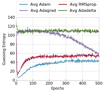
When the model training dataset is large, the cost of gradient descent for each
iteration will be high. For additional information about optimizers, we refer
interested readers to [4].
    SGD. Stochastic gradient descent is a stochastic approximation of the gradi-
ent descent algorithm that minimizes the objective function written as a sum of
differentiable functions. SGD reduces computational cost at each iteration as it
uniformly samples an index i ∈ 1, . . . , N at random and computes the gradient
to update θ (one update of parameters for each training example). Due to the
frequent updates with a high variance for SGD, this can cause large fluctuations
of the loss function. Instead of taking only a single example to update the pa-
rameters, we can also take a fixed number of them: a mini-batch. In that case,
we talk about mini-batch SGD.
    Momentum. SGD can have problems converging around the local optima
due to the shape of the surface curves. Momentum (also called classical mo-
mentum) is a technique that can help alleviate this and accelerate SGD in the
relevant direction. It does this by adding a fraction γ (momentum term) of the
update vector of the past time step to the current update vector. The momen-
tum term increases for dimensions whose gradients point in the same directions
and reduces updates for dimensions whose gradients change directions.
    Nesterov. Nesterov (Nesterov accelerated gradient) improves upon momen-
tum by approximating the next position of the parameters. More precisely, we
can calculate the gradient for the approximate future position of parameters.
This anticipatory step prevents momentum from going too fast, increasing the
performance of the neural network.
    Adagrad. Adagrad adapts the learning rate to the parameters, performing
smaller updates (small learning rates) for parameters associated with frequently
occurring features, and larger updates (high learning rates) for parameters as-
sociated with less frequent features. One of Adagrad’s main benefits is that it
eliminates the need to tune the learning rate manually. On the other hand, dur-
ing the training process, the learning rates shrink (due to the accumulation of the
squared gradients), up to the point where the algorithm cannot obtain further
knowledge.
    Adadelta. Adadelta represents an extension of the Adagrad method. In
Adadelta, we aim to reduce its monotonically decreasing learning rate. More
precisely, instead of accumulating all past squared gradients, Adadelta restricts
the window of accumulated past gradients to some fixed size. The sum of gradi-
ents is recursively defined as a decaying average of all past squared gradients to
avoid storing those squared gradients.
    RMSprop. RMSprop is an adaptive learning rate method that aims to re-
solve Adagrad’s aggressively decreasing learning rates (like Adadelta). RMSprop
divides the learning rate by an exponentially decaying average of squared gradi-
ents.
    Adam. Adam (Adaptive Moment Estimation) is one more method that com-
putes adaptive learning rates for each parameter. This method combines the
benefits of Adagrad and RMSprop methods. This way, it stores an exponentially

                                        5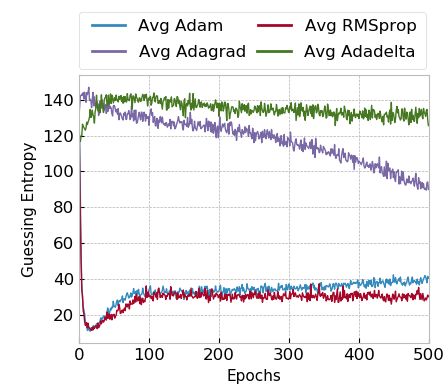
decaying average of past squared gradients, but it also keeps an exponentially
decaying average of past gradients, which is similar to the momentum method.

2.3   Datasets

We consider two publicly available datasets, representing software AES im-
plementations protected with the first-order Boolean masking - the ASCAD
database [24]. The traces were measured from an implementation consisting of
a software AES implementation running on an 8-bit microcontroller. The AES
is protected with the first-order masking, where the two first key bytes (index
1 and 2) are not protected with masking (e.g., masks set to zeros) and the key
bytes 3 to 16 are masked.
    The first dataset is the ASCAD dataset with the fixed key. For the data
with fixed key encryption, we use a time-aligned dataset in a prepossessing step.
There are 60 000 EM traces (50 000 training/cross-validation traces and 10 000
test traces), and each trace consists of 700 points of interest (POI).
    For the second dataset, we use ASCAD with random keys, where there are
200 000 traces in the profiling dataset and 100 000 traces in the attack dataset.
A window of 1 400 points of interest is extracted around the leaking spot. We
use the raw traces and the pre-selected window of relevant samples per trace
corresponding to masked S-box for i = 3.
    The first dataset can be considered as a small dataset, while the second one is
large. This difference is important for the performance of the optimizers, as seen
in the next sections. Since the ASCAD dataset leaks mostly in the Hamming
weight leakage model, we consider it in our experiments. The ASCAD dataset
is available at https://github.com/ANSSI-FR/ASCAD.

3     Related Works

In recent years, the number of works considering machine learning (and espe-
cially deep learning) in SCA has grown rapidly. This is not surprising as most of
those works report excellent attack performance and breaking targets protected
with countermeasures [2,11]. From a wide plethora of available deep learning
techniques, multilayer perceptron and convolutional neural networks are com-
monly used and achieve top performance. To achieve such top results, one needs
to (carefully) tune the neural network architecture. We can informally divide
research works based on the amount of attention that the tuning takes. Indeed,
the first works do not discuss how detailed tuning is done, or even what are the
final hyperparameters selected [7,9].
    More recently, researchers give more attention to the tuning process, and
they report the best settings selected from a wide pool of tested options. To find
such good hyperparameters, common choices are random search, grid search,
or grid search within specific ranges [24,23,20]. A more careful look at those
works reveals that most of the attention goes toward the architecture hyperpa-
rameters [24], and only rarely toward the training process hyperparameters [13].

                                        6
What is more, those works commonly conduct hyperparameter tuning as the
necessary but less “interesting” step, which means there are no details about
performance for various settings nor how difficult it was to find good hyperpa-
rameters. Still, we note works are investigating how to find a good performing
neural network [31], but even then, the training process hyperparameters receive
less attention. Differing from those works, we 1) concentrate on the hyperparam-
eter tuning process, and 2) investigate the optimizer hyperparameter as one of
the essential settings of the training process. First, in Section 4, we concentrate
on the influence of optimizers regardless of the selection of other hyperparameters
(thus, we present averaged results over numerous profiled models). In Section 5,
we investigate the influence of optimizers on specific neural network architec-
tures.

4   The General Behavior of Optimizers in Profiled SCA

To understand the influence of optimizers, we analyze the results based on GE’s
evolution concerning the number of epochs. Note that such an analysis is com-
putationally very expensive, as it requires to calculate GE for every epoch. Ad-
ditionally, to explore the influence of optimizers in combination with the archi-
tecture size, we divide the architectures into small (less than 400 000 trainable
parameters) and large (more than 1 000 000 trainable parameters).
    As shown next, the selection of an optimizer in SCA mostly depends on the
model size and the regularization (implicit or explicit). What is more, most re-
lated works use Adam or RMSprop in MLP or CNN architectures. This choice
is possibly related to the nature of the attacked dataset and the fast conver-
gence provided by these two optimizers. Moreover, we also demonstrate that the
capacity of a model to generalize (here, generalization is measured with GE of
correct key byte candidate) or overfit is directly related to implicit and explicit
regularization. Implicit regularization can be provided by the optimization al-
gorithm itself or by the model size concerning the number of profiling traces.
Smaller models trained on larger datasets show implicit regularization, and the
models tend to generalize better. On the other hand, larger models, even on
larger datasets, tend to provide less implicit regularization, allowing the model
to overfit very fast. The results in this section are obtained from a random hy-
perparameter search, both for MLPs and CNNs. Tables 1 and 2 in Appendix B
specify the range of hyperparameters we investigated. To calculate the average
GE, we run the experiments for 1 000 independent profiled models, and then we
average those results.
    All results show the ASCAD dataset results for fixed key or random keys. In
the first case, there are 50 000 traces in the profiling phase. The guessing entropy
is computed from a separate test set of 1 000 traces, having a fixed key. For the
ASCAD random key datasets, it consists of 200 000 training traces with random
keys, while the attack phase uses 2 000 traces with a fixed key.

                                         7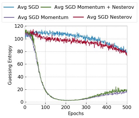
4.1   Stochastic Gradient Descent Optimizers
We tested SGD optimizer in four different configurations: SGD, SGD with Nes-
terov, SGD with momentum (0.9), and SGD with both momentum (0.9) and
Nesterov. Note that we take the default value for the momentum.
    Figures 1a and 1b show results for guessing entropy for the ASCAD fixed key
for small and large models, respectively. Figures 2a and 2b provide results for
the guessing entropy evolution for the ASCAD random keys datasets, for small
and large models, respectively.

         (a) Small Models                     (b) Large Models

   Fig. 1: SGD optimizers and model size for the ASCAD fixed key dataset.

         (a) Small Models                     (b) Large Models

 Fig. 2: SGD optimizers and model size for the ASCAD random keys dataset.

   Results for both datasets for SGD optimizers indicate that SGD performs
better on small and large datasets when momentum is considered. Without mo-

                                      8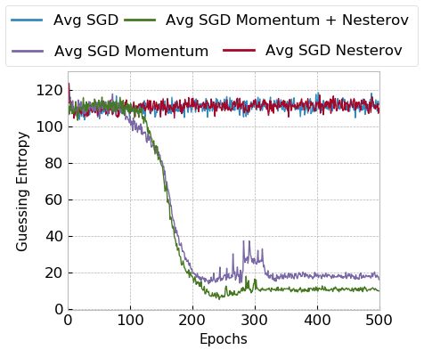
mentum, we verified that SGD performs relatively better for large models, espe-
cially when Nesterov is applied. Moreover, we observe that SGD with momentum
tends to perform better for large datasets and large models, as seen in Figure 2b.
Additionally, for ASCAD with a fixed key, we observe a slower convergence for
small models but no overfitting. On the other hand, for large models, SGD
with momentum reaches top performance around epoch 150, and afterward, GE
increases, indicating model overfit. For ASCAD with random keys, we do not
observe overfitting even if using large models, which is a clear indication that
random keys make the classification problem more difficult, and the model needs
more capacity to fit the data. Interestingly, small models show a similar trend
for the ASCAD fixed key dataset, demonstrating that such models already reach
the top of their capacity for the simpler dataset.
4.2 Adaptive Gradient Descent Methods
In [30], the authors analyze the empirical generalization capability of adaptive
methods. They conclude that overparameterized models can easily overfit with
adaptive optimizers. As demonstrated in [14], adaptive optimizers such as Adam
and RMSprop display faster progress in the initial portion of training, and the
performance usually degrades if the number of training epochs is too large. As
a consequence, the model overfits. This leaves the need for additional (explicit)
regularization in order to overcome the overfitting.
We analyze the behavior of adaptive optimizers for profiled SCA, and we
show that the easy overfitting of adaptive methods reported in [30] happens for
Adam and RMSprop, but not for Adagrad and Adadelta. In particular, we show
that Adagrad and Adadelta tend to work better for larger models and longer
training times.
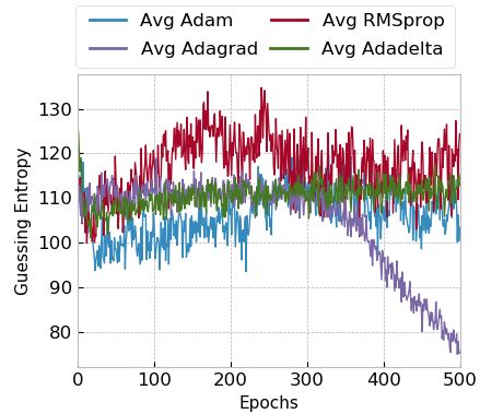
Figures 3a and 3b show the averaged guessing entropy results for the ASCAD
with fixed key for small and large models, respectively. Figures 4a and 4b show
GE evolution during training for small and large models for ASCAD with random
keys.
The general behavior of guessing entropy evolution during training with
adaptive optimizers is similar for both datasets, indicating that this could be
a typical optimizer behavior regardless of the attacked dataset. Adam and RM-
Sprop usually converge very fast. In these cases, guessing entropy for correct key
candidates tends to drop to a low value (under 20) when the model can pro-
vide some level of generalization. However, after the guessing entropy reaches its
minimum value (i.e., maximum generalization), the processing of more epochs
does not benefit and only degrades the model generalization. This means that
Adam optimizer tends to overfit very fast, and early stopping would be highly
beneficial to deal with this problem. A long training process is not beneficial
when Adam optimizer is considered for profiled SCA. RMSprop tends to work
less efficiently than Adam for larger models and larger datasets.
Adagrad provides a slighter decrease in guessing entropy if the model can
provide some generalization. Unlike Adam and RMSprop, it does not degrade
the guessing entropy with the processing of more epochs, which indicates that a
9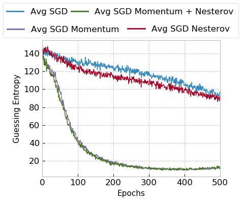
(a) Small Models                      (b) Large Models

 Fig. 3: Adaptive optimizers and model size for the ASCAD fixed key dataset.

          (a) Small Models.                     (b) Large Models.

Fig. 4: Adaptive optimizers and model size for the ASCAD random keys dataset.

long training process is beneficial when Adagrad is selected as an optimization
algorithm. Normally, generalization can happen very late in the training process,
which means that a larger number of epochs might be necessary for Adagrad.
Adadelta shows less capacity to generalize in different deep neural network con-
figurations. Like Adagrad, once the generalization starts to occur, it does not
degrade with the processing of more epochs. Generalization can start very late in
the training process. Our results indicate that Adagrad should be the optimizer
of choice, especially if using larger models (thus, if expecting that the dataset is
difficult, so we require large profiled model capacity) and, uncertain how to tune
other hyperparameters. Besides the above observations, we also verified that, on
average, MLPs tend to provide a faster convergence (faster dropping in guess-
ing entropy) for Adam and RMSprop in comparison to CNNs for the ASCAD

                                        10
random keys dataset. On the other hand, for Adagrad and Adadelta, we did not
observe a significant difference in performance for MLPs and CNNs.
5 Optimizers and Specific Profiled Models
In the previous section, we provided averaged different optimizers behaviors if
other hyperparameters are randomly selected. This type of analysis can indicate
the typical behavior of the optimizers independently of the rest of the hyper-
parameters. We aim to confirm if a fixed neural network architecture can show
specific behavior for different optimizers, i.e., whether the selection of optimizer
influences another hyperparameter. For that, we define small and large MLPs
as well as small and large CNNs. All neural network models (MLP or CNN)
are trained with a batch size of 400, a learning rate of 0.001, and default Keras
library initialization for weight and biases.
The small MLP and CNN models are defined as follows:
– A small MLP: four hidden layers, each having 200 neurons.
– A small CNN: one convolutional layer (10 filters, kernel size 10, and stride
10) and two fully-connected layers with 200 neurons.
– A large MLP: ten hidden layers, each having 1000 neurons.
– A large CNN: four convolutional layers (10, 20, 40, and 80 filters, kernel size
4, and stride 2 in all the four convolutional layers) and four fully-connected
layers with 1 000 neurons each.
The output layers for MLP and CNN contain nine neurons (the Hamming
Weight leakage model) with the Softmax activation function. Unless specified
otherwise, all neural networks have the RelU activation function in all the layers.
For adaptive optimizers and large profiled models, we also provide results for
the ELU activation function. We train these neural networks on both ASCAD
datasets, with fixed and random keys in the training data. For every neural
network and dataset, we run the analysis ten times (10 experiments with the
same architecture) and then average GE results from these ten executions.
5.1 SGD Optimizers on Small MLP and CNN
Shallow neural networks with only a few hidden layers implement learning mod-
els with a relatively small number of trainable parameters. As a result, a large
amount of training data would hardly overfit these models. Thus, a small model
implements an implicit regularization given by its reduced capacity to com-
pletely fit the training data. Empirical results observed in this work lead us to
conclude that some optimizers pose no additional regularization effect on the
learning process, while some other optimizers present a more significant implicit
regularization.
The behaviors of SGD optimizers on a small MLP and a small CNN are
shown in Figures 5 and 6. Without momentum, SGD shows limited capacity to
learn side-channel leakages. For CNN, GE for the scenario without momentum
remains at the same level during the processing of 500 epochs. For MLP, we see
11(a) ASCAD fixed key. (b) ASCAD random keys.
Fig. 5: SGD optimizers on small MLP models.
(a) ASCAD fixed key. (b) ASCAD random keys.
Fig. 6: SGD optimizers on small CNN models.
a small convergence, indicating that the model can learn without momentum.
However, it takes a large number of epochs. When momentum, with or without
Nesterov, is considered, we observe a smooth convergence of the guessing entropy
during training for small MLP and small CNN. When the training set is larger,
as is the case of the ASCAD random keys dataset, the convergence is slightly
faster. To conclude, we can assume that small MLP and CNN models with SGD
as the optimizer requires momentum to improve model learnability. What is
more, we see that we generally require a large number of epochs to converge
to small GE (observing related works, most of them do not consider such long
training processes).
5.2 SGD Optimizers on Large MLP and CNN
Again, SGD optimizers on large models present better performance when mo-
mentum is used, either with or without Nesterov. As for CNN models, without
12momentum, GE stays around the same level during the whole training. Although
large MLP models show better capacity to fit side-channel leakage for SGD with-
out momentum, the results from Figures 7 and 8 show once more that SGD works
much better with momentum in the side-channel context.
(a) ASCAD fixed key. (b) ASCAD random keys.
Fig. 7: SGD optimizers on large MLP models.
(a) ASCAD fixed key. (b) ASCAD random keys.
Fig. 8: SGD optimizers on large CNN models.
Note, that the results observed in Figures 7 and 8 for the SGD optimizers
with momentum are representative of the recently described behavior of neural
networks called the deep double descent [18]. Interestingly, these results indicate
that longer training phases, larger profiled models, or more training examples do
not necessarily improve the classification process. The results first show conver-
gence (decrease of GE), after which there is a GE increase, and then, again, GE
13decreases (thus, double descent). Interestingly, comparing the results for small
and large models shows that the final GE values are very similar. This means
that it makes more sense to invest extra computational time into longer training
phases than larger models.
5.3 Adaptive Optimizers on Small MLP and CNN
From adaptive optimizers, results indicate that Adam and RMSprop are the
only ones that provide successful attack results, as the guessing entropy drops
consistently in the first epochs, as indicated by Figures 9a and 9b on the ASCAD
fixed key and ASCAD random keys, respectively. On the other hand, Adagrad
and Adadelta cannot provide GE decrease during training, emphasizing that
these optimizers do not work well for small models.
(a) ASCAD fixed key. (b) ASCAD random keys.
Fig. 9: Adaptive optimizers on small MLP model.
As expected, for the model trained on the ASCAD fixed key, containing 50 000
training traces, the guessing entropy evolution for Adam and RMSprop increases
after the processing of 50 epochs. For the ASCAD random keys scenario, where
200 000 traces are used for training, the increase in GE for Adam and RMSprop
is less distinct. Consequently, small models with larger training sets tend to
work well for Adam and RMSprop optimizers. However, these two optimizers
require additional regularization mechanisms to ensure that the model is not
over-trained. In the results provided in Figures 9a and 9b, early stopping would
be a good alternative, as already discussed [19,26].
As shown in Figures 10a and 10b, Adam and RMSprop also provided faster
guessing entropy convergence for a small CNN model. Adagrad shows slightly
better results for a small CNN compared to a small MLP, indicating that this
type of adaptive optimizer may provide successful attack results if the number
of epochs is very large (guessing entropy decreases up to epoch 500). For the
Adadelta optimizer, a small CNN model shows no convergence at all.
14(a) ASCAD fixed key. (b) ASCAD random keys.
Fig. 10: Adaptive optimizers on small CNN model.
5.4 Adaptive Optimizers on Large MLP and CNN
Here, we observe different behavior for adaptive optimizers and different acti-
vation functions. Adam and RMSprop tend to show poor performance in com-
parison to small MLP models, especially when ELU is selected as the activation
function, as shown in Figure 11b. For the ReLU activation function (see Fig-
ure 11a), which is commonly employed in state-of-art neural network architec-
tures, these two optimizers tend to perform relatively better, even though they
are very sensitive to overfitting, as GE increases if the amount of training epochs
is too large.
For Adagrad and Adadelta, we observed that a large MLP performs rela-
tively well if ELU activation function is selected for hidden layers, as shown in
Figure 11b. In this case, the network requires more training epochs to converge
to a low guessing entropy (approx. 400 epochs in Figure 11b). The advantage
of Adagrad and Adadelta with large MLP models and ELU is that guessing
entropy stays low even if the number of epochs is very large (e.g., 500 epochs).
Results for the four studied adaptive optimizers for large MLP on ReLU and
ELU activation functions are shown in Figures 11a and 11b, respectively.
Similar behavior is observed for the ASCAD fixed key dataset. Figures 12a
and 12b show results for a large MLP model with ReLU and ELU activation
functions, respectively. As the analysis in this section suggests, large MLP mod-
els work better with Adagrad and Adadelta as optimizers and ELU activation
function. For Adam and RMSprop cases, even carefully selecting the activation
function was insufficient to achieve a stable convergence of guessing entropy
during training. Once more, we verify that Adam and RMSprop may provide
better performance by adding extra regularization artifacts, such as early stop-
ping. When the training set consists of a small number of measurements, as is
the case of the ASCAD fixed key dataset, Adam and RMSprop tend to provide
a narrow generalization interval. As Figure 12a shows, low guessing entropy for
Adam and RMSprop last for less than 10 epochs and after that, guessing entropy
15(a) ReLU. (b) ELU.
Fig. 11: Adaptive optimizers on large MLP models for the ASCAD with random
keys.
only increases. For larger training sets, as provided by the ASCAD random keys
dataset, the interval in which guessing entropy is low is wider, as seen in the
example of Figure 11b. In this case, the guessing entropy remains low until at
least the processing of 50 epochs.
(a) ReLU. (b) ELU.
Fig. 12: Adaptive optimizers on large MLP models for the ASCAD fixed key
dataset.
As shown in Figures 13 and 14, Adagrad shows superior performance for
large CNN models with ELU activation function in a long training process. This
is even more clear in Figure 13b where large CNN is trained on a large dataset.
Although Figures 13b and 14b show guessing entropy convergence for Adam
and RMSprop in the first epochs, a large CNN model seems to provide worse
16performance than a large MLP for these two adaptive optimizers. One possible
explanation for this behavior could be that large CNNs simply have too large
capacity and cannot conduct sufficient feature selection for a good attack. For
Adadelta, we observed a slow GE convergence after 400 epochs in the scenario
illustrated in Figure 13b. Besides that, Adadelta provided no promising results
in the evaluated large CNN.
(a) ReLU. (b) ELU.
Fig. 13: Adaptive optimizers on large CNN models for the ASCAD random keys
dataset.
(a) ReLU. (b) ELU.
Fig. 14: Adaptive optimizers on large CNN models for the ASCAD fixed key
dataset.
176 Conclusions
The selection of an optimizer algorithm for the training process during the pro-
filed SCA has a significant influence on the attack results. In this work, we
provide results for eight different optimizers, separated into adaptive and SGD
groups. We verified that Adam and RMSprop optimizers show better perfor-
mance when the neural network is small, and the training process is short. The
adaptive Adagrad and Adadelta show good performance when large models are
considered. Additionally, we confirmed that the selection of adaptive optimizer
strictly depends on the activation function for hidden layers.
In future work, we plan to investigate the behavior of different optimizers
and identity value leakage model. Besides that, in this work, we concentrate
on two datasets only. To confirm our findings, we aim to extend the analysis
with more publicly available datasets. Finally, we are interested in exploring the
double descent behavior in SCA. While we observed that longer training does
not necessarily mean better performance, we are interested in observing that
larger models are not necessarily better or that larger profiling phases improve
the behavior.
References
1. Brier, E., Clavier, C., Olivier, F.: Correlation power analysis with a leakage model.
In: Joye, M., Quisquater, J.J. (eds.) Cryptographic Hardware and Embedded Sys-
tems - CHES 2004. pp. 16–29. Springer Berlin Heidelberg, Berlin, Heidelberg (2004)
2. Cagli, E., Dumas, C., Prouff, E.: Convolutional Neural Networks with Data Aug-
mentation Against Jitter-Based Countermeasures - Profiling Attacks Without Pre-
processing. In: Cryptographic Hardware and Embedded Systems - CHES 2017 -
19th International Conference, Taipei, Taiwan, September 25-28, 2017, Proceed-
ings. pp. 45–68 (2017)
3. Chari, S., Rao, J.R., Rohatgi, P.: Template attacks. In: International Workshop on
Cryptographic Hardware and Embedded Systems. pp. 13–28. Springer (2002)
4. Choi, D., Shallue, C.J., Nado, Z., Lee, J., Maddison, C.J., Dahl, G.E.: On empirical
comparisons of optimizers for deep learning (2019)
5. Collobert, R., Bengio, S.: Links Between Perceptrons, MLPs and SVMs.
In: Proceedings of the Twenty-first International Conference on Ma-
chine Learning. pp. 23–. ICML ’04, ACM, New York, NY, USA (2004).
https://doi.org/10.1145/1015330.1015415, http://doi.acm.org/10.1145/
1015330.1015415
6. Gierlichs, B., Batina, L., Tuyls, P., Preneel, B.: Mutual information analysis. In:
Oswald, E., Rohatgi, P. (eds.) Cryptographic Hardware and Embedded Systems –
CHES 2008. pp. 426–442. Springer Berlin Heidelberg, Berlin, Heidelberg (2008)
7. Gilmore, R., Hanley, N., O’Neill, M.: Neural network based attack on a
masked implementation of aes. In: 2015 IEEE International Symposium on
Hardware Oriented Security and Trust (HOST). pp. 106–111 (May 2015).
https://doi.org/10.1109/HST.2015.7140247
8. Hettwer, B., Gehrer, S., Güneysu, T.: Deep neural network attribution meth-
ods for leakage analysis and symmetric key recovery. In: Paterson, K.G.,
18Stebila, D. (eds.) Selected Areas in Cryptography - SAC 2019 - 26th In-
ternational Conference, Waterloo, ON, Canada, August 12-16, 2019, Revised
Selected Papers. Lecture Notes in Computer Science, vol. 11959, pp. 645–
666. Springer (2019). https://doi.org/10.1007/978-3-030-38471-5 26, https://
doi.org/10.1007/978-3-030-38471-5_26
9. Heuser, A., Picek, S., Guilley, S., Mentens, N.: Side-channel analysis of lightweight
ciphers: Does lightweight equal easy? In: Hancke, G.P., Markantonakis, K. (eds.)
Radio Frequency Identification and IoT Security. pp. 91–104. Springer Interna-
tional Publishing, Cham (2017)
10. Heuser, A., Zohner, M.: Intelligent Machine Homicide - Breaking Cryptographic
Devices Using Support Vector Machines. In: Schindler, W., Huss, S.A. (eds.)
COSADE. LNCS, vol. 7275, pp. 249–264. Springer (2012)
11. Kim, J., Picek, S., Heuser, A., Bhasin, S., Hanjalic, A.: Make some noise. un-
leashing the power of convolutional neural networks for profiled side-channel anal-
ysis. IACR Transactions on Cryptographic Hardware and Embedded Systems
2019(3), 148–179 (May 2019). https://doi.org/10.13154/tches.v2019.i3.148-179,
https://tches.iacr.org/index.php/TCHES/article/view/8292
12. Kocher, P.C., Jaffe, J., Jun, B.: Differential power analysis. In: Proceedings of
the 19th Annual International Cryptology Conference on Advances in Cryptology.
pp. 388–397. CRYPTO ’99, Springer-Verlag, London, UK, UK (1999), http://dl.
acm.org/citation.cfm?id=646764.703989
13. Li, H., Krcek, M., Perin, G.: A comparison of weight initializers in deep learning-
based side-channel analysis. IACR Cryptol. ePrint Arch. 2020, 904 (2020), https:
//eprint.iacr.org/2020/904
14. Luo, L., Xiong, Y., Liu, Y., Sun, X.: Adaptive gradient methods with dynamic
bound of learning rate. In: 7th International Conference on Learning Representa-
tions, ICLR 2019, New Orleans, LA, USA, May 6-9, 2019. OpenReview.net (2019),
https://openreview.net/forum?id=Bkg3g2R9FX
15. Maghrebi, H., Portigliatti, T., Prouff, E.: Breaking cryptographic implementations
using deep learning techniques. In: Security, Privacy, and Applied Cryptography
Engineering - 6th International Conference, SPACE 2016, Hyderabad, India, De-
cember 14-18, 2016, Proceedings. pp. 3–26 (2016)
16. Mangard, S., Oswald, E., Popp, T.: Power Analysis Attacks: Revealing the Se-
crets of Smart Cards. Springer (December 2006), ISBN 0-387-30857-1, http:
//www.dpabook.org/
17. Masure, L., Dumas, C., Prouff, E.: Gradient visualization for general char-
acterization in profiling attacks. In: Polian, I., Stöttinger, M. (eds.) Con-
structive Side-Channel Analysis and Secure Design - 10th International
Workshop, COSADE 2019, Darmstadt, Germany, April 3-5, 2019, Proceed-
ings. Lecture Notes in Computer Science, vol. 11421, pp. 145–167. Springer
(2019). https://doi.org/10.1007/978-3-030-16350-1 9, https://doi.org/10.1007/
978-3-030-16350-1_9
18. Nakkiran, P., Kaplun, G., Bansal, Y., Yang, T., Barak, B., Sutskever, I.: Deep dou-
ble descent: Where bigger models and more data hurt. In: 8th International Confer-
ence on Learning Representations, ICLR 2020, Addis Ababa, Ethiopia, April 26-30,
2020. OpenReview.net (2020), https://openreview.net/forum?id=B1g5sA4twr
19. Perin, G., Buhan, I., Picek, S.: Learning when to stop: a mutual information
approach to fight overfitting in profiled side-channel analysis. Cryptology ePrint
Archive, Report 2020/058 (2020), https://eprint.iacr.org/2020/058
1920. Perin, G., Chmielewski, L., Picek, S.: Strength in numbers: Improving generaliza-
tion with ensembles in profiled side-channel analysis. Cryptology ePrint Archive,
Report 2019/978 (2019), https://eprint.iacr.org/2019/978
21. Picek, S., Heuser, A., Jovic, A., Bhasin, S., Regazzoni, F.: The curse of
class imbalance and conflicting metrics with machine learning for side-channel
evaluations. IACR Trans. Cryptogr. Hardw. Embed. Syst. 2019(1), 209–
237 (2019). https://doi.org/10.13154/tches.v2019.i1.209-237, https://doi.org/
10.13154/tches.v2019.i1.209-237
22. Picek, S., Heuser, A., Jovic, A., Ludwig, S.A., Guilley, S., Jakobovic, D., Mentens,
N.: Side-channel analysis and machine learning: A practical perspective. In: 2017
International Joint Conference on Neural Networks, IJCNN 2017, Anchorage, AK,
USA, May 14-19, 2017. pp. 4095–4102 (2017)
23. Picek, S., Samiotis, I.P., Kim, J., Heuser, A., Bhasin, S., Legay, A.: On the perfor-
mance of convolutional neural networks for side-channel analysis. In: Chattopad-
hyay, A., Rebeiro, C., Yarom, Y. (eds.) Security, Privacy, and Applied Cryptogra-
phy Engineering. pp. 157–176. Springer International Publishing, Cham (2018)
24. Prouff, E., Strullu, R., Benadjila, R., Cagli, E., Dumas, C.: Study of deep learning
techniques for side-channel analysis and introduction to ascad database. Cryptol-
ogy ePrint Archive, Report 2018/053 (2018), https://eprint.iacr.org/2018/053
25. Quisquater, J.J., Samyde, D.: Electromagnetic analysis (ema): Measures and
counter-measures for smart cards. In: Attali, I., Jensen, T. (eds.) Smart Card
Programming and Security. pp. 200–210. Springer Berlin Heidelberg, Berlin, Hei-
delberg (2001)
26. Robissout, D., Zaid, G., Colombier, B., Bossuet, L., Habrard, A.: Online perfor-
mance evaluation of deep learning networks for side-channel analysis. Cryptology
ePrint Archive, Report 2020/039 (2020), https://eprint.iacr.org/2020/039
27. Schindler, W., Lemke, K., Paar, C.: A stochastic model for differential side chan-
nel cryptanalysis. In: International Workshop on Cryptographic Hardware and
Embedded Systems. pp. 30–46. Springer (2005)
28. Standaert, F.X., Malkin, T., Yung, M.: A Unified Framework for the Analysis
of Side-Channel Key Recovery Attacks. In: EUROCRYPT. LNCS, vol. 5479, pp.
443–461. Springer (April 26-30 2009), Cologne, Germany
29. Weissbart, L.: On the performance of multilayer perceptron in profiling side-
channel analysis. Cryptology ePrint Archive, Report 2019/1476 (2019), https:
//eprint.iacr.org/2019/1476
30. Wilson, A.C., Roelofs, R., Stern, M., Srebro, N., Recht, B.: The marginal value
of adaptive gradient methods in machine learning. In: Guyon, I., von Luxburg,
U., Bengio, S., Wallach, H.M., Fergus, R., Vishwanathan, S.V.N., Garnett, R.
(eds.) Advances in Neural Information Processing Systems 30: Annual Con-
ference on Neural Information Processing Systems 2017, 4-9 December 2017,
Long Beach, CA, USA. pp. 4148–4158 (2017), http://papers.nips.cc/paper/
7003-the-marginal-value-of-adaptive-gradient-methods-in-machine-learning
31. Zaid, G., Bossuet, L., Habrard, A., Venelli, A.: Methodology for effi-
cient cnn architectures in profiling attacks. IACR Transactions on Cryp-
tographic Hardware and Embedded Systems 2020(1), 1–36 (Nov 2019).
https://doi.org/10.13154/tches.v2020.i1.1-36, https://tches.iacr.org/index.
php/TCHES/article/view/8391
20A Machine Learning Classifiers
We consider two neural network types that are standard techniques in the pro-
filed SCA: multilayer perceptron and convolutional neural networks.
Multilayer Perceptron. The multilayer perceptron (MLP) is a feed-forward
neural network that maps sets of inputs onto sets of appropriate outputs. MLP
consists of multiple layers of nodes in a directed graph, where each layer is fully
connected to the next one (thus, layers are called fully-connected or dense lay-
ers). An MLP consists of three or more layers (since input and output represent
two layers) of nonlinearly-activating nodes [5].
Convolutional Neural Networks. Convolutional neural networks(CNNs)
are feed-forward neural networks commonly consisting of three types of layers:
convolutional layers, pooling layers, and fully-connected layers. The convolution
layer computes neurons’ output connected to local regions in the input, each
computing a dot product between their weights and a small region connected to
the input volume. Pooling decrease the number of extracted features by perform-
ing a down-sampling operation along the spatial dimensions. The fully-connected
layer (the same as in multilayer perceptron) computes either the hidden activa-
tions or the class scores.
B Neural Networks Hyperparameter Ranges
In Table 1, we show the hyperparameter ranges we explore for the MLP archi-
tectures, while in Table 2, we show the hyperparameter ranges for CNNs.
Hyperparameter min max step
Learning Rate 0.0001 0.01 0.0001
Mini-batch 400 1 000 100
Dense (fully-connected) layers 1 10 1
Neurons (for dense layers) 100 1 000 10
Activation function (all layers) ReLU, Tanh, ELU, or SELU
Table 1: Hyperparameter search space for multilayer perceptron.
21Hyperparameter min max step
Learning Rate 0.0001 0.01 0.0001
Mini-batch 400 1 000 100
Convolution layers 1 4 1
Convolution Filters 4*l 8*l 1
Convolution Kernel Size 1 40 1
Convolution Stride 1 4 1
Dense (fully-connected) layers 1 10 1
Neurons (for dense layers) 100 1 000 10
Activation function (all layers) ReLU, Tanh, ELU, or SELU
Table 2: Hyperparameters search space for convolutional neural network (l =
convolution layer index).
22You can also read