Robust Digital Molecular Design of Binarized Neural Networks
←
→
Page content transcription
If your browser does not render page correctly, please read the page content below
Robust Digital Molecular Design of Binarized
Neural Networks
Johannes Linder         #
University of Washington, Paul G. Allen School of Computer Science and Engineering,
Seattle, WA, USA

Yuan-Jyue Chen
Microsoft Research, Redmond, WA, USA

David Wong
University of Washington, Department of Bioengineering, Seattle, WA, USA

Georg Seelig
University of Washington, Paul G. Allen School of Computer Science and Engineering,
Seattle, WA, USA
University of Washington, Department of Electrical and Computer Engineering,
Seattle, WA, USA

Luis Ceze
University of Washington, Paul G. Allen School of Computer Science and Engineering,
Seattle, WA, USA

Karin Strauss
Microsoft Research, Redmond, WA, USA
University of Washington, Paul G. Allen School of Computer Science and Engineering,
Seattle, WA, USA

      Abstract
Molecular programming – a paradigm wherein molecules are engineered to perform computation –
shows great potential for applications in nanotechnology, disease diagnostics and smart therapeutics.
A key challenge is to identify systematic approaches for compiling abstract models of computation
to molecules. Due to their wide applicability, one of the most useful abstractions to realize is
neural networks. In prior work, real-valued weights were achieved by individually controlling
the concentrations of the corresponding “weight” molecules. However, large-scale preparation of
reactants with precise concentrations quickly becomes intractable. Here, we propose to bypass this
fundamental problem using Binarized Neural Networks (BNNs), a model that is highly scalable in
a molecular setting due to the small number of distinct weight values. We devise a noise-tolerant
digital molecular circuit that compactly implements a majority voting operation on binary-valued
inputs to compute the neuron output. The network is also rate-independent, meaning the speed at
which individual reactions occur does not affect the computation, further increasing robustness to
noise. We first demonstrate our design on the MNIST classification task by simulating the system
as idealized chemical reactions. Next, we map the reactions to DNA strand displacement cascades,
providing simulation results that demonstrate the practical feasibility of our approach. We perform
extensive noise tolerance simulations, showing that digital molecular neurons are notably more
robust to noise in the concentrations of chemical reactants compared to their analog counterparts.
Finally, we provide initial experimental results of a single binarized neuron. Our work suggests a
solid framework for building even more complex neural network computation.

2012 ACM Subject Classification Theory of computation → Models of computation; Applied
computing

Keywords and phrases Molecular Computing, Neural Network, Binarized Neural Network, Digital
Logic, DNA, Strand Displacement

Digital Object Identifier 10.4230/LIPIcs.DNA.27.1
            © Johannes Linder, Yuan-Jyue Chen, David Wong, Georg Seelig, Luis Ceze, and Karin Strauss;
            licensed under Creative Commons License CC-BY 4.0
27th International Conference on DNA Computing and Molecular Programming (DNA 27).
Editors: Matthew R. Lakin and Petr Šulc; Article No. 1; pp. 1:1–1:20
                   Leibniz International Proceedings in Informatics
                   Schloss Dagstuhl – Leibniz-Zentrum für Informatik, Dagstuhl Publishing, Germany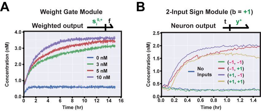
1:2   Robust Digital Molecular Neural Networks

       1     Introduction
      Computing in molecules is a prerequisite for a wide range of potentially revolutionizing
      nanotechnologies, such as molecular nanorobots and smart therapeutics. For example,
      molecular “programs” delivered to cells could collect sensory input from gene expression
      to determine the prevalence of disease and conditionally release a drug. Molecular disease
      classifiers have already been demonstrated outside of cells [1, 18]. Moreover, as researchers
      look toward synthetic DNA for storing data [9, 20, 4], it becomes increasingly important to
      develop operations that can be executed on data in molecular form.
          Bringing such applications closer to reality requires abstractions and programming
      languages that can capture the desired molecular behaviors. A methodical way to reason
      about chemical computing is through the formalism of chemical reaction networks (CRNs).
      A CRN is a collection of coupled chemical reactions, each consuming a set of reactants to
      create a set of products. CRNs are Turing universal [27, 12] and any CRN can in principle be
      implemented using synthetic DNA molecules, specifically DNA strand displacement [28, 7].
          Molecular computing has traditionally been approached from two different design philo-
      sophies; in analog computing, the numerical value of each variable is encoded in the concen-
      tration of its corresponding molecular species [24, 5, 33]. Conversely, in digital molecular
      computing, concentrations of species representing logical values are restricted to “high” or
      “low” ranges similar to voltages in digital electronics [13, 19]. Feed-forward neural networks
      have previously been demonstrated as analog molecular circuits [34, 23, 6, 8, 32]. While
      compact, analog molecular circuits are inherently sensitive to concentration noise, as such
      perturbation directly impacts the correctness of the system.
          Here, we develop a digital molecular implementation of binarized neural networks, a
      class of models where the inputs, weights and activations are constrained to take the
      values {+1, −1} [14]. We devise an efficient molecular circuit for computing binary n-input
      majority using O(n2 ) gates and O(logn) (optimal) depth. Each neuron uses this circuit
      for their weighted sum and threshold operation. This design offers a uniquely scalable
      molecular implementation: while an analog monotonic network requires exponentially large
      concentrations of molecular substrates as a function of layer depth to avoid saturation of
      outputs (we develop this argument in Section 3), our design uses a constant concentration
      across all network layers. We demonstrate our design on the MNIST task, both as idealized
      CRNs and as DNA strand displacement cascades. Finally, we compare the digital neuron to
      an analog, rate-independent HardTanh-activated neuron and present improved robustness to
      concentration noise and leak. We also present initial experimental results of a simple 2-input
      binarized neuron.

       2     Background

      2.1    Binarized Neural Networks
      In this paper we focus on deterministic binarized neural networks (BNNs) as described by [14].
      If we first consider a single neuron, its inputs xi , weights wi , bias term b and activation y
      are binary-valued and constrained to {+1, −1}. We compute neuron activation y as:
               (            PN
                 +1 if b + i=1 wi · xi > 0
          y=                                                                                      (1)
                 −1 else

      Binarized neurons are assembled into fully connected neural networks by treating output
      y of a neuron i in layer k as the input xi to neuron j of layer k + 1, connected through
               (k)
      weight wij ∈ {+1, −1}. BNNs can be efficiently trained by gradient descent following the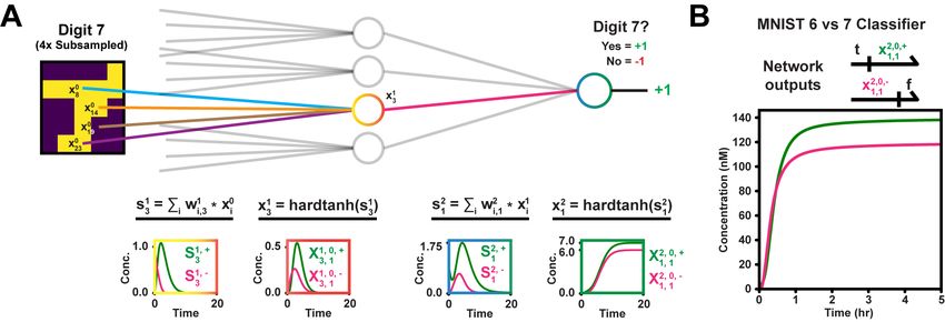
J. Linder, Y.-J. Chen, D. Wong, G. Seelig, L. Ceze, and K. Strauss 1:3
scheme of the original authors, where a straight-through estimator was used to propagate
gradients through binarized non-linearities. While BNNs usually are less accurate than their
full-precision counterparts, they offer substantial improvements in execution time and storage
space [26]. Since BNN computation can be executed with bitwise operations, they are also
amenable to efficient implementation on FPGAs and ASICs. Recent BNN architectures show
relatively good performance on more complex tasks such as ImageNet classification [10].
2.2 Chemical Reaction Networks
Chemical Reaction Networks (CRNs) are a mathematical formalism traditionally used by
chemists to describe how the concentration or counts of chemical species evolve over time.
Two example reactions are shown below:
A+B →C
C →D+E
Reaction 1 dictates that one molecule each of A and B react to produce C, until A or B are
fully consumed. Reaction 2 consumes one molecule of C to produce one molecule each of D
and E. Commonly, a rate constant that captures how fast an instance of a reaction occurs is
also associated with each reaction. In this paper, we consider reactions with at most two
reactants or two products. When modeling the time evolution of CRNs, we often reason
about concentrations. We denote the concentration of A at time t as a(t). Assuming mass
action kinetics, a(t) can be modeled as an ODE [11].
Analog and Digital CRNs
Molecular programming with CRNs can be approached from different computational models.
Two of the most widely used models are analog CRNs and digital CRNs. In analog CRNs,
any non-negative real-valued variable x ∈ R+ is represented by a corresponding molecular
species X. The value of x is encoded in the concentration x(t) [24]. For example, x = 3.2 is
represented as x(t) = 3.2nM. This convention makes summation trivial to implement; to
PN
compute s = i=1 xi , we add N reactions translating species Xi to the same species S:
Xi → S ,1≤i≤N
As time progresses, each input Xi accumulates in species S such that t → ∞ s(t) =
PN
i=1 xi (0).
In a digital computing paradigm, we restrict variables to be discrete, such that they can
only take on a finite number of states. Each discrete variable and state is encoded by its
own molecular species (e.g. Boolean variable x is encoded by two species, X (on) and X (off) ).
Chemical concentrations represent only high or low signals indicating which state is active.
For example, Boolean variable x is modeled by the following CRN convention (Here T (high) is
a constant representing the signal filter cutoff and the third case represents incorrect states):
on
if x(on) (t) ≥ T (high) and x(off) (t) < T (high)
x = off if x(on) (t) < T (high) and x(off) (t) ≥ T (high)
(undefined) else
Note that N -input summation is more complicated under this paradigm, as inputs can no
longer simply be translated to the same output species to encode logical sum. Instead, proper
digital circuits such as carry adders have been implemented as CRNs [16, 22].
DNA 271:4 Robust Digital Molecular Neural Networks
Piecewise Linear CRNs and HardTanh
In analog CRNs, a real-valued variable x ∈ R that can take on negative values is often
represented in dual-rail form by two species X − and X + . The value of x is encoded as
the difference in their concentration, x = limt→∞ x+ (t) − x− (t). Using this convention, the
function h = max(x, −k) can be implemented by two reactions [5] (the initial concentration
of K is set to k(0) = k and x+ (0), x− (0) are initialized such that x+ (0) − x− (0) = x):
X+ → H+ + K
X− + K → H− (2)
Similarly, function y = min(h, m) can be implemented as (here m(0) = m etc.):
H− → Y − + M
H+ + M → Y + (3)
Note that k, m ∈ R+ , so dual-rail is not needed to express their values. By stacking these two
sets of reactions and setting k(0) = 1 and m(0) = 1, we can implement a rate-independent,
analog HardTanh function, y = min(max(x, −1), 1). We use this construction below when
comparing the digital neuron developed in this paper to a HardTanh-activated neuron based
on analog CRNs, which is similar to the ReLU (Rectified Linear Unit) network by [32].
2.3 DNA Strand Displacement
Toehold-mediated DNA strand displacement (DSD) is a framework capable of synthesizing
any CRN [28, 7, 30]. Molecular species are compiled into signal strands which react through
synthetic DNA gates as specified by the CRN reactions. In this paper we use the two-domain
architecture from [3], which supports all of the functionality needed to implement our digital
BNN design; the gates can be prepared at large scale from double-stranded DNA by enzymatic
processing and the architecture supports AND-logic, catalytic amplification and fan-out
operations.
Two-domain gates work by exposing a toehold which, when hybridized by an input strand,
triggers a sequence of displacements. These displacements ultimately release the output
strand bound to the gate. As an example, consider the simple CRN reaction A → B. The
corresponding two-domain DSD system is shown in Figure 1. Species A is represented by the
signal strand to the left (domains t and a – abbreviated ta) and B is represented by the strand
with domains b and f (bf ). A sequence of displacements mediated by toehold t eventually
releases the output strand from the gate. Specifically, the sequence of displacements are:
1. Input strand ta binds to gate G, displacing strand at and exposing inner toehold t.
(Reversible reaction)
2. Helper strand tb binds to the newly opened toehold, displacing output strand bf and
exposing inner toehold f. (Reversible reaction)
3. Helper strand fw binds to the newly opened toehold, displacing strand w and closing gate
G. (Irreversible reaction)
A promising alternative for synthesizing CRNs is Polymerase-mediated strand displace-
ment (PSD), where polymerase enzymes trigger initially single-stranded DNA gates by
extending hybridized input strands and consequently displacing any output strand [29, 25].
In this paper, we focus solely on implementing the neural network with enzyme-free toehold-
mediated DSD, but we discuss implementation with PSD towards the end.J. Linder, Y.-J. Chen, D. Wong, G. Seelig, L. Ceze, and K. Strauss 1:5
Figure 1 Input strand ta releases strand at and exposes new toehold t. Additional steps of strand
displacement (not shown) ultimately release output strand bf. Additional helper strands tb and fw
(not shown) help carry out the sequence of displacement reactions.
3 Related Work
Neural networks with real-valued weights based on analog computation have previously been
built with DNA strand displacement cascades [23, 8, 6]. Non-linear activation was achieved
by introducing threshold gates with much faster reaction rates than gates producing an
output signal. A recent paper by [32] proposed a rate-independent analog CRN to implement
a neural network with binary-valued weights and ReLU activations.
Neural networks based on monotonic analog CRNs may require exponentially large
concentrations of molecular substrates at deeper network layers to avoid saturation. To
see why, assume a binary-weighted, ReLU-activated network consisting of K layers and
k
N neurons per layer. If we set all weights wij to +1 and all inputs x0i to +1, then each
activation in the first layer becomes:
N
X
x1j = max 0
· x0i , 0 = N.
wij
i=1
To physically implement this computation, we require a DSD gate or other substrate that can
produce the molecular species for x1j at a concentration N times larger than x0i . Inductively, at
the final layer, each activation xK K
j can be as large as N , requiring gates with concentrations
K
proportional to N to avoid saturation. We can similarly construct a worst-case example
k
for the HardTanh function from the previous section; by setting half the weights wij to +1
+ −
and half the weights to −1, the concentration of output species Y / Y of Reaction Set 3
will be N/2. With the same inductive argument as before, we need gate concentrations
proportional to (N/2)K to avoid saturation.
Our design differs from that of [23] and [32] in that the CRN computation is carried out
with digital logic. Since concentrations are used only to represent high or low signals, the
computation remains correct under perturbation, similar in concept to how electronic digital
circuits offer more robust behavior than analog electronic circuits. The digital design also
makes the system rate-independent and allows for a uniform gate concentration across all
network layers.
4 A Digital Molecular Implementation of Binarized Neurons
A binarized neuron with inputs xi ∈ {+1, −1}, weights wi ∈ {+1, −1} and bias b ∈ {+1, −1}
is illustrated in Figure 2A. To simplify the implementation, we assume the number of inputs,
N , is a power of 2. The neuron consists of a sequence of three operations:
1. Weight operations s0i = wi · xi , where s0i denotes weighted input i before summation.
PN
2. A sum operation s = i=1 s0i .
3. A sign operation y = sign(s + b), where b breaks ties in the case when s = 0.
DNA 271:6 Robust Digital Molecular Neural Networks
Alternatively, steps 2 and 3 may be considered a majority voting operation between positive
and negative inputs. The following sections describe how we implement the computational
graph shown in Figure 2B of a digital neuron with chemical reactions. We only discuss a
single neuron here to keep the notation light, but a generalization to an arbitrarily sized
BNN is described in Appendix A.
4.1 Weight
Each input xi is represented by two CRN species, Xi+ and Xi− , corresponding to states
xi = +1 and xi = −1 respectively. We implement the weight operation s0i = wi · xi as follows
(Figure 2C): If wi = +1, we add catalytic reactions translating the positive-state input
species Xi+ to the positive-state weighted species Si0,+ , and we similarly translate Xi− to
Si0,− .
Xi+ → Xi+ + Si0,+
Xi− → Xi− + Si0,−
If wi = −1, we instead translate Xi+ to Si0,− , and vice versa for the negative-state input
species.
Xi+ → Xi+ + Si0,−
Xi− → Xi− + Si0,+
In practice, the catalytic reactions do not replenish the input species indefinitely, but rather
transform some gate substrate G into waste W (e.g. X + G → X + W + Y for input species
X and output Y ), but this does not matter for our theoretical analysis.
4.2 Majority Vote
If there are more weighted species s0i = wi · xi in a positive state than a negative state, the
circuit should output a positive state, and vice versa. We can easily enumerate every such
rule as a chemical reaction of N-ary AND-clauses, given the CRN species Si0,+ and Si0,− of
each weighted input. For example, to handle the case s0 = w ∗ x = (+1, +1, +1, −1), we
would add the reaction:
S10,+ + S20,+ + S30,+ + S40,− → Y +
This CRN is problematic for two reasons: First, the number of reactions grows exponentially
with N . Second, the CRN requires arbitrary-length AND-clauses, which is not feasible when
implemented as DNA strand displacement gates. Instead, we here devise an efficient digital
majority voting CRN that requires only a quadratic number of gates and a logarithmic
PN
(optimal) depth. We will compute the sum s = i=1 s0i as a balanced tree of binary additions
using a recursive definition (Figure 2B):
k−1
skh = s2h−1 + sk−1
2h
Here k = 1, ..., log(N ) and h = 1, ..., N/2k . At level k = log(N ), the full sum s is stored
log(N )
in s1 . For each binary addition performed during the recursion, we will add chemical
reactions translating every possible combination of discrete values of sk−1 k−1
2h−1 and s2h into
k
the species of sh corresponding to their sum. Suppose the summands can take on m discreteJ. Linder, Y.-J. Chen, D. Wong, G. Seelig, L. Ceze, and K. Strauss 1:7
Figure 2 A Illustration of a binarized neuron. B Computational graph of a binarized neuron.
The binary summation tree (blue) has a depth of log(N ). C Chemical reactions which implement
the modules of the computational graph. D Example illustration of the binary addition circuit. A
set of AND rules encode which input states (summands) correspond to what output state (sum).
k−1,v1 k−1,vm
values, sk−1 k−1
2h−1 , s2h ∈ {v1 , ..., vm }. We represent these states with species S2h−1 , ..., S2h−1
k−1,v1 k−1,vm
and S2h , ..., S2h . For every combination of values vi , vj , add the following reaction
(Figure 2C):
k−1,vi k−1,vj k,vi +vj
S2h−1 + S2h → Sh
Example logical circuits are illustrated in Figure 2D for m = 2 and m = 3. In general, if
the input variables have cardinality m, we require m2 reactions and the cardinality of the
output variable becomes 2m − 1. Note that this circuit is more similar to a demultiplexer
than a carry adder.
Since each binary addition has depth 1, and there are log(N ) levels of additions, the
total depth is log(N ). To calculate the total number of reactions, we first note that, at
level k, there are N/2k additions. Each summand has cardinality m = 2k−1 + 1 (assuming
binary-valued initial inputs). Hence, the total number of reactions across all log(N ) levels
can be calculated as a geometric series:
DNA 271:8 Robust Digital Molecular Neural Networks
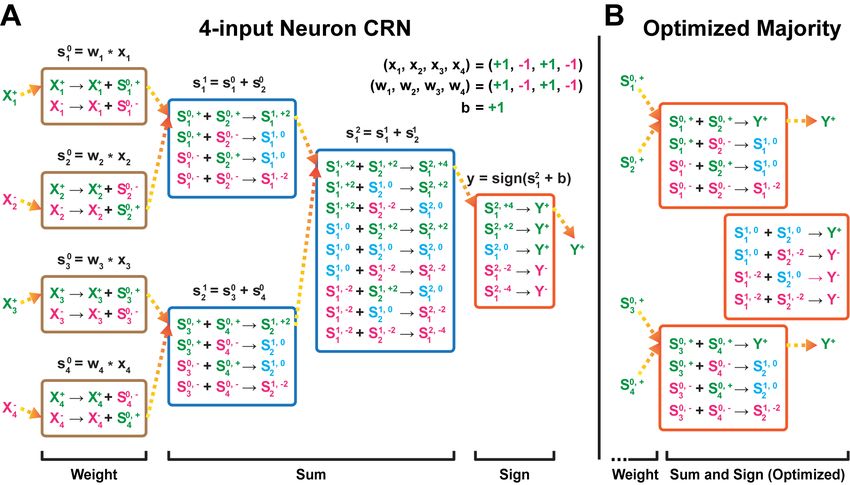
Figure 3 A Example CRN execution of a 4-input neuron. (x1 , x2 , x3 , x4 ) = (+1, −1, +1, −1) and
(w1 , w2 , w3 , w4 ) = (+1, −1, +1, −1). B Optimized 4-input neuron (weight reactions are omitted).
log(N ) log(N )−1
X (2k−1 + 1)2 X 22k + 2k+1 + 1
N· =N·
2k 2k
k=1 k=0
N2 N
= + N · log(N ) + −1
2 2
= O(N 2 )
We have thus shown that we can construct a digital sum circuit as a balanced binary tree
of chemical reactions with O(log(N )) depth and O(N 2 ) reactions. We finalize the majority
voting circuit by adding uni-molecular reactions translating every possible state species
log(N ),−N log(N ),+N log(N )
S1 , ..., S1 of the final sum s1 into the correct signed output species Y +
or Y − (N reactions):
log(N ),v
S1 → Y sign(v+b)
4.3 An Illustrative Example: A 4-Input Binarized Neuron
We show the digital CRN of a 4-input binarized neuron in Figure 3A, which carries out the
full sum before applying the sign reaction. However, we are ultimately not interested in
computing the sum of input species, only their majority vote. If the absolute value of the
partial sum in any of the sub trees is greater than N/2, we can stop computing the sum
since the majority is already determined. That is, if |vi + vj + b| > N/2, alter the reaction to
immediately produce the output species Y + or Y − :
k−1,vi k−1,vj
S2h−1 + S2h → Y sign(vi +vj +b)J. Linder, Y.-J. Chen, D. Wong, G. Seelig, L. Ceze, and K. Strauss 1:9
Table 1 Number of CRN reactions required to compute N -input digital majority.
N 2 4 8 16 32
# Reactions 4 12 50 182 654
Similarly, it is unnecessary to translate the final sums into their corresponding signs with
separate uni-molecular reactions; we can immediately produce the output species Y + , Y −
from the last level of sums. An optimized 4-input binarized neuron is illustrated in Figure 3B.
The optimization reduces the input cardinality of the two summands at the final level by 1.
Using the geometric series defined in Section 4.2, we can calculate the number of removed
reactions at level k = log(N ):
(2log(N )−1 + 1)2 (2log(N )−1 )2
N· log(N )
−N · =N +1
2 2log(N )
2
The optimized circuit thus requires N2 + N · log(N ) − N2 − 2 reactions to compute digital
majority. Table 1 lists the number of required reactions up to N = 32 inputs.
4.4 DNA Strand Displacement Design
Here we present the DNA strand displacement (DSD) implementation of the digital BNN
CRN. The implementation is based on the two-domain design of [3]. The complete DSD
schematic is shown in Figure 4. The implementation is described in detail below.
Each activation xli in layer l is represented by two input strands, Xil,+ and Xil,− . For
each weighted connection sl,0 l l−1 l
i,j = wi,j · xi , we add four gates. If wi,j = +1, we add the
following gates:
1. Gate Gl,+ l−1,+
Weight,i,j , which outputs Ki
l,0,+
and Si,j given the strand Xil−1,+ as input.
2. Gate Gl−1,+ l−1,+
Restore,i , which translates Ki back to Xil−1,+ .
3. Gate Gl,− l−1,+
Weight,i,j , which outputs Ki
l,0,−
and Si,j given the strand Xil−1,+ as input.
4. Gate Gl−1,− l−1,−
Restore,i , which translates Ki back to Xil−1,− .
l l,0,+ l,0,−
If wi,j = −1, we swap the output strands Si,j and Si,j such that they are released
l,− l,+
by gates GWeight,i,j and GWeight,i,j respectively. Next, we add a cascade of AND gates to
PN l−1
implement slj = i=1 sl,0 l,k l,k−1 l,k−1
i . For each binary addition sh,j = s2h−1,j + s2h,j , for all M
2
combinations of summand values vm1 , vm2 , we add:
l,k,m1 ,m2 l,k,vm1 +vm2 l,k−1,v l,k−1,vm2
1. Gate GSum,h,j , which outputs Sh,j given S2h−1,j m1 and S2h,j as input.
However, if k = log(N l−1 ) (the final tree level), or if |sl,k−1 l,k−1 l
2h−1,j + s2h,j + bj | > N
l−1
/2, we let
Gl,k,m 1 ,m2
Sum,h,j produce the neuron majority species Xjl,+ or Xjl,− .
Note that, since the output strand of each two-domain gate reverses orientation as
compared to its input strand(s) (the toehold moves to the opposite side of the recognition
domain), we have to alternate the orientation of gates at each level in the summation tree.
Also, since the summation can end at either an odd or- even numbered level, we have to add
translator gates which swap the orientation of the final activation species Xjl,+ and Xjl,− .
This guarantees that the activation output strands are always in the correct orientation with
respect to the input weight gates of the next layer.
DNA 271:10 Robust Digital Molecular Neural Networks
Figure 4 DSD schematic of the binarized neural network implementation, based on the two-
domain architecture of [3].J. Linder, Y.-J. Chen, D. Wong, G. Seelig, L. Ceze, and K. Strauss 1:11
Figure 5 A A single-hidden layer network with 4, 8 or 12 neurons was trained to classify MNIST
digits 6 vs. 7. B Example CRN simulation, as a system of ODEs with unit concentrations and
reaction rates. Graph color corresponds to network component. C The network was simulated in
Microsoft’s DSD tool. Signal concentration = 20nM. Shown is the final output strand trajectory.
5 Experiments
5.1 MNIST Simulations
We demonstrate our binarized neural network design on the MNIST digit classification task.
Similar to one of the analyses in [8], we tested the model’s ability to distinguish between
digits 6 and 7. We trained three versions of a single-hidden layer network (Figure 5A),
with 4, 8 and 12 hidden neurons respectively. For the 4 and- 8 hidden neuron networks, we
downsampled the input images to 5 × 5 pixels. For the 12 neuron version, the images were
downsampled to 10 × 10 pixels. The image pixel values were binarized by subtracting the
mean pixel intensity and thresholding at 0. We settled on a sparse connectivity structure,
where neurons were connected to 4 randomly chosen inputs. The networks were trained
following the procedure of [14], using PyTorch [21] and the Adam optimizer [15].
The network with only 4 hidden neurons correctly classified as many as 93% of test
images (Figure 5A, bottom table). Test accuracy increased marginally up to 96% for the
largest network. We translated the 4-hidden neuron network into our digital CRN design,
totalling 192 molecular species and 102 reactions, and simulated the entire system of ODEs
for an example input image (Figure 5B). Finally, we mapped the 4-hidden neuron network
CRN to a DNA strand displacement (DSD) cascade, using the architecture presented in
Section 4.4. The DSD specification was compiled into a system of ODEs using Microsoft’s
DSD tool with default toehold binding rates and “infinite” compilation mode [17]. The ODE
was simulated by Python SciPy’s odeint (Figure 5B).
5.2 Noise Tolerance Simulations
Next, we compared our digital design (d-BNN) to an analog rate-independent design (a-BNN)
with the HardTanh activation function defined in Section 2.2. The designs were compiled
into CRNs using Microsoft’s DSD tool. Each CRN was copied to Python, compiled into
ODEs and simulated by SciPy’s odeint. Keeping the designs as CRNs in Python allows us
to easily add leak pathways. We provide the schematic for the analog HardTanh network as
idealized CRNs in Appendix B and as DNA strand displacement cascades in Appendix C.
DNA 271:12 Robust Digital Molecular Neural Networks
Figure 6 A A single 4-input neuron was compiled into DSD (both as a digital circuit – d-BNN,
and as an analog circuit – a-BNN). Shown is the tested input pattern. B Noise- and leak tolerance
simulations. Concentrations varied uniformly between 0.5x-2x or 0.25x-4x. Signal concentration
(1x) = 20nM. Leak reactions were added to DSD gates with rates of 10−8 or 10−7 nM−1 s−1 . Each
simulation was run 10 times. 95% confidence intervals estimated from 1000-fold bootstrapping.
We compared the effects of concentration noise and gate leak on each respective design
for a single 4-input neuron (Figure 6A). Specifically, we multiplied input strand and gate
concentrations with a uniform random value and added leak reactions to all gates. Four
different conditions were tested, and each condition was simulated 10 times. The results
indicate that the digital binarized neuron is more robust than its analog counterpart (Fig-
ure 6B); in all four conditions, the correct “turned-on” output trajectory is separable from
the “turned-off” (leaked) trajectory up to 3 hours for the digital neuron, whereas the analog
neuron looses separability of the output trajectories almost immediately.
5.3 Physical Experimental Results
We performed wet lab experiments to validate the function of the basic DSD components
used in the BNN. In Figure 7A, we tested a single catalytic two-domain weight gate, which
is used to restore the input signal to the operating concentration (4nM) given different
concentrations of input strand. As can be seen, the gate restores the signal with low levels of
leak, and all conditions reach 75% of the target concentration within 12 hours. In Figure 7B,
we tested the function of a simple 2-input majority voter where the bias term b is set to +1.
The experiment suggests that the system functions correctly with low levels of leak. Note
that there is no catalytic amplification of the majority voting output signal in Figure 7B,
which is why the concentration is not restored to 4nM.
6 Discussion
When comparing digital BNNs to other molecular neural network implementations, our design
offers both advantages and disadvantages. In terms of complexity, our design is less efficient
(compact) than both rate-dependent and rate-independent analog designs [23, 8, 32], which
require O(N ) bi-molecular reactions for weighting and only O(1) reactions for majority voting.
However, our simulations indicate that the digital design is more robust to concentration noise
and gate leak compared to analog implementations. Furthermore, since rate-independent
analog CRNs operate on monotonic dual-rail species, any physical implementation of aJ. Linder, Y.-J. Chen, D. Wong, G. Seelig, L. Ceze, and K. Strauss 1:13
Figure 7 A An amplifier is used to restore the operating concentration (4nM) of the input strand
given different input strand concentrations. B A 2-input majority voting circuit with +1 bias is used
to trigger the output strand only if the positive inputs are in majority. Input concentration is 4nM.
deep, fully connected neural network would require an exponentially large concentration of
molecular substrates at the final network layers (exponential in the network layers). The
digital design, however, allows a constant substrate concentration across all layers.
The DSD architecture of the digital BNN can potentially support even large networks,
since the DNA gates can be enzymatically prepared from a pool of fully double-stranded
DNA [7]. However, it is often difficult in practice to scale up the number of two-domain gates
in a single reaction vessel due to the many possible leak pathways, in particular for catalytic
gates. To reduce noise, we might consider isolating each neuron computation with either
localized reactions [2] or physical separation by microfluidic droplets [31]. Alternatively,
strand-displacing polymerase (PSD) may be a promising option, which leak minimally [29, 25].
Furthermore, all reactions can be implemented with single-stranded PSD AND-gates, allowing
for simple large-scale synthesis. The main caveat is that PSD currently does not support
catalytic reactions. However, we can forego the catalytic reactions and instead start with
exponentially large input concentrations, which may be feasible for 1–2 hidden layers of
computation.
Finally, for future work we wonder whether the gate complexity of O(N 2 ) for digital
majority voting can be reduced by acknowledging that neural networks often behave well
with small errors. We thus ask if we could design an “approximate” majority voter with
O(N ) gates. For example, instead of computing exact partial sums on groups of inputs, we
might get approximately correct output using only the signs of the inputs at each level of
the tree.
7 Conclusion
In this paper, we present a digital molecular design of binarized neural networks. We devise
a depth-optimal majority voting circuit that uses O(N 2 ) bi-molecular chemical reactions in
a cascade of depth O(log(N )) to compute N -input majority. Each neuron uses this circuit
to compute its activation function. We demonstrated our molecular implementation on the
MNIST digit classification task, by simulating the ODE of a network with 4 hidden neurons
as a DNA strand displacement cascade. We further demonstrated improved tolerance to
concentration noise compared to analog BNN implementations in simulations.
We hope this paper sparks future research in molecular implementations of machine
learning models. The intersection of digital circuit design, ML techniques and chemical
reaction networks can enable other computational models implemented as molecular circuits
and lead to whole new applications in molecular computing.
DNA 271:14 Robust Digital Molecular Neural Networks
References
1 Y. Benenson, B. Gil, U. Ben-Dor, R. Adar, and E. Shapiro. An autonomous molecular
computer for logical control of gene expression. Nature, 429(6990):423–429, 2004.
2 H. Bui, S. Shah, R. Mokhtar, T. Song, S. Garg, and J. Reif. Localized DNA hybridization
chain reactions on DNA origami. ACS nano, 12(2):1146–1155, 2018.
3 L. Cardelli. Two-domain DNA strand displacement. Mathematical Structures in Computer
Science, 23(2):247–271, 2013.
4 L. Ceze, J. Nivala, and K. Strauss. Molecular digital data storage using dna. Nature Reviews
Genetics, 20(8):456–466, 2019.
5 H.L. Chen, D. Doty, and D. Soloveichik. Rate-independent computation in continuous chemical
reaction networks. In Proceedings of the 5th Conference on Innovations in Theoretical Computer
Science, pages 313–326, 2014 January.
6 S.X. Chen and G. Seelig. A DNA neural network constructed from molecular variable gain
amplifiers. In International Conference on DNA-Based Computers, pages 110–121, 2017
September.
7 Y.J. Chen, N. Dalchau, N. Srinivas, A. Phillips, L. Cardelli, D. Soloveichik, and G. Seelig.
Programmable chemical controllers made from DNA. Nature nanotechnology, 8(10):755–762,
2013.
8 K.M. Cherry and L. Qian. Scaling up molecular pattern recognition with DNA-based winner-
take-all neural networks. Nature, 559(7714):370–376, 2018.
9 G.M. Church, Y. Gao, and S. Kosuri. Next-generation digital information storage in DNA.
Science, 337(6102):1628–1628, 2012.
10 S. Darabi, M. Belbahri, M. Courbariaux, and V.P. Nia. BNN+: Improved binary network
training. OpenReview, 2018.
11 I.R. Epstein and J.A. Pojman. An introduction to nonlinear chemical dynamics: Oscillations,
waves, patterns, and chaos. Oxford Univ Press London, page London, 1998.
12 F. Fages, G. Le Guludec, O. Bournez, and A. Pouly. Strong turing completeness of continuous
chemical reaction networks and compilation of mixed analog-digital programs. In International
Conference on Computational Methods in Systems Biology, pages 108–127, 2017 September.
13 A. Hjelmfelt, E.D. Weinberger, and J. Ross. Chemical implementation of neural networks and
turing machines. Proceedings of the National Academy of Sciences, 88(24):10983–10987, 1991.
14 I. Hubara, M. Courbariaux, D. Soudry, R. El-Yaniv, and Y. Bengio. Binarized neural networks.
In Advances in Neural Information Processing Systems, pages 4107–4115, 2016.
15 D.P. Kingma and J. Ba. Adam: A method for stochastic optimization. arXiv, 2014. arXiv:
1412.6980.
16 M.R. Lakin and A. Phillips. Modelling, simulating and verifying turing-powerful strand
displacement systems. In International Workshop on DNA-Based Computers, pages 130–144,
2011 September.
17 M.R. Lakin, S. Youssef, F. Polo, S. Emmott, and A. Phillips. Visual DSD: a design and
analysis tool for DNA strand displacement systems. Bioinformatics, 27(22):3211–3213, 2011.
18 R. Lopez, R. Wang, and G. Seelig. A molecular multi-gene classifier for disease diagnostics.
Nature chemistry, 10(7):746–754, 2018.
19 M.O. Magnasco. Chemical kinetics is turing universal. Physical Review Letters, 78(6):1190,
1997.
20 L. Organick, S.D. Ang, Y.J. Chen, R. Lopez, S. Yekhanin, K. Makarychev, M.Z. Racz,
G. Kamath, P. Gopalan, B. Nguyen, and C.N.etal. Takahashi. Random access in large-scale
DNA data storage. Nature biotechnology, 36(3):242, 2018.
21 A. Paszke, S. Gross, S. Chintala, G. Chanan, E. Yang, Z. DeVito, Z. Lin, A. Desmaison,
L. Antiga, and A. Lerer. Automatic differentiation in pytorch, 2017.
22 L. Qian and E. Winfree. Scaling up digital circuit computation with DNA strand displacement
cascades. Science, 332(6034):1196–1201, 2011.J. Linder, Y.-J. Chen, D. Wong, G. Seelig, L. Ceze, and K. Strauss 1:15
23 L. Qian, E. Winfree, and J. Bruck. Neural network computation with DNA strand displacement
cascades. Nature, 475(7356):368–372, 2011.
24 P. Senum and M. Riedel. Rate-independent constructs for chemical computation. PloS one,
6(6):e21414, 2011.
25 S. Shah, J. Wee, T. Song, L. Ceze, K. Strauss, Y.J. Chen, and J. Reif. Using strand displacing
polymerase to program chemical reaction networks. Journal of the American Chemical Society,
142(21):9587–9593, 2020.
26 T. Simons and D.J. Lee. A review of binarized neural networks. Electronics, 8(6):661, 2019.
27 D. Soloveichik, M. Cook, E. Winfree, and J. Bruck. Computation with finite stochastic
chemical reaction networks. Natural Computing, 7(4):615–633, 2008.
28 D. Soloveichik, G. Seelig, and E. Winfree. DNA as a universal substrate for chemical kinetics.
Proceedings of the National Academy of Sciences, 107(12):5393–5398, 2010.
29 T. Song, A. Eshra, S. Shah, H. Bui, D. Fu, M. Yang, R. Mokhtar, and J. Reif. Fast and
compact DNA logic circuits based on single-stranded gates using strand-displacing polymerase.
Nature nanotechnology, 14(11):1075–1081, 2019.
30 N. Srinivas, J. Parkin, G. Seelig, E. Winfree, and D. Soloveichik. Enzyme-free nucleic acid
dynamical systems. Science, 358(6369), 2017.
31 A. Stephenson, M. Willsey, J. McBride, S. Newman, B. Nguyen, C. Takahashi, K. Strauss, and
L. Ceze. PurpleDrop: A digital microfluidics-based platform for hybrid molecular-electronics
applications. IEEE Micro, 40(5):76–86, 2020.
32 M. Vasic, C. Chalk, S. Khurshid, and D. Soloveichik. Deep molecular programming: A natural
implementation of binary-weight ReLU neural networks. arXiv, 2020. arXiv:2003.13720.
33 M. Vasic, D. Soloveichik, and S. Khurshid. CRN++: Molecular programming language. In
International Conference on DNA Computing and Molecular Programming, pages 1–18, 2018
October.
34 D.Y. Zhang and G. Seelig. DNA-based fixed gain amplifiers and linear classifier circuits. In
International Workshop on DNA-Based Computers, pages 176–186, 2010 June.
A Generalized CRN Definition for Multi-layered Digital BNN
In this appendix, we extend the CRN formalism defined in Section 4 from a single binarized
neuron to an arbitrarily sized network consisting of multiple neurons across many layers.
Let us first extend the notation of the in-silico computational model, which, to remind the
reader, is based on deterministic binarized neural networks (BNNs) as described by [14] with
the added constraint that the number of neurons in any layer is a power of 2.
Let L be the number of network layers and let N l be the number of neurons in layer l.
(l)
Define xi ∈ {+1, −1} as the binary-valued activation of neuron i in layer l or, if l = 0, let
(0)
xi be the i:th input to the network. Neuron i in layer l − 1 is connected to neuron j of
(l)
layer l through the binary-valued weight wi,j ∈ {+1, −1}. Additionally, Neuron j of layer l
(l) (l)
has an associated bias term (intercept) bj ∈ {+1, −1}. We define activation xj of neuron
j recursively as:
(
(l) PN l−1 (l) (l−1)
(l) +1 if bj + i=1 wi,j · xi >0
xj =
−1 else
CRN Definition
Each neuron activation xli is represented by two CRN species Xil,+ and Xil,− , corresponding
to states xli = +1 and xli = −1 respectively. For each weight operation sl,0 l l−1
i,j = wi,j · xi , add
l
either of the following sets of reactions based on the sign of wi,j :
DNA 271:16 Robust Digital Molecular Neural Networks
l
If wi,j = +1:
l,0,+
Xil−1,+ → Xil−1,+ + Si,j
Xil−1,− → Xil−1,− + Si,j
l,0,−
l
Else if wi,j = −1:
l,0,−
Xil−1,+ → Xil−1,+ + Si,j
Xil−1,− → Xil−1,− + Si,j
l,0,+
PN l−1
The sum operation slj = i=1 sl,0 i is calculated as a balanced tree of binary additions using
the following recursive definition:
sl,k l,k−1 l,k−1
h,j = s2h−1,j + s2h,j
Here k = 1, ..., log(N l−1 ) denotes the current depth in the tree and h = 1, ..., N l−1 /2k
denotes the tree node. Assume each summand can take on M discrete values, sl,k−1 l,k−1
2h−1,j , s2h,j ∈
{v1 , ..., vM }. The resulting sum can take on 2M −1 values, sl,k
h,j ∈ {v1 +v1 , v1 +v2 , ..., vM +vM }.
We represent each discrete state of each variable with a distinct molecular species:
State sl,k l,k,vm
h,j = vm is encoded by species Sh,j
For each of the M 2 combinations of summand values sl,k−1 l,k−1
2h−1,j = vm1 , s2h,j = vm2 , add the
reaction:
l,k−1,v l,k−1,vm2 l,k,vm1 +vm2
S2h−1,j m1 + S2h,j → Sh,j
l,log(N l−1 )
At depth log(N l−1 ) in the tree, the final weighted sum will be stored in variable s1,j .
To compute the binary threshold activation function of neuron j in layer l, which we represent
with species Xjl,+ and Xjl,− , add the following reaction for each of the N + 1 possible sum
l,log(N ),−N l,log(N ),+N
output species S1,j , ..., S1,j (recalling that blj is the bias term for neuron j in
layer l):
l,log(N ),v l,sign(v+blj )
S1,j → Xj
B Analog Rate-Independent HardTanh Network CRN
In the main paper, we compare the digital CRN of a binary-threshold neuron to an analog
CRN implementation of a HardTanh-activated neuron. Here, we describe the analog design,
including idealized CRN reactions and the two-domain DSD schematic. The implementation
is based on the rate-independent neural network CRN that was recently proposed by [32],
but with a HardTanh activation function min(max(x, −1), 1) instead of the ReLU function
max(x, 0).
In analog CRN computing, the weight and- sum operations are performed simultaneously.
We implement the weighted sum of neuron j,
l−1
N
X
slj = l
wi,j · xli
i=1
by adding either of the following two sets of reactions for each input i:J. Linder, Y.-J. Chen, D. Wong, G. Seelig, L. Ceze, and K. Strauss 1:17
l
If wi,j = +1:
l−1,log(N l ),+
Xi,j → Sjl,+
l−1,log(N l ),−
Xi,j → Sjl,−
l
Else if wi,j = −1:
l−1,log(N l ),+
Xi,j → Sjl,−
l−1,log(N l ),−
Xi,j → Sjl,+
Note that the molecular species for input xl−1 i are indexed by j. We cannot use catalytic
reactions for rate-independent monotonic CRNs, which means we have to make individual
copies of xl−1
i for each outgoing neuron j. Further down in this text, we will add fan-out
reactions which create as many copies of xlj as needed by the next layer. This copy operation,
which is implemented as a binary tree, is the reason for having the hard-coded superscript
log(N l ) in the species notation. Also note that the bias term blj is implemented by setting
the initial concentrations of Sjl,+ and Sjl,− appropriately; if blj = +1, start with sl,+
j (0) = 1,
l l,−
or if bj = −1, start with sj (0) = 1.
Next, we implement the HardTanh activation function,
xlj = min(max(slj , −1), 1)
by stacking the monotonic, dual-rail reaction set of the two functions hlj = max(slj , −k) and
xlj = min(hlj , m) as described by [5]:
Sjl,+ → Hjl,+ + Kjl
Sjl,− + Kjl → Hjl,−
Hjl,− → Xj,1
l,0,−
+ Mjl
Hjl,+ + Mjl → Xj,1
l,0,+
In order for these reactions to implement clipping of slj at [-1, 1], we have to start with initial
concentrations kjl (0) = 1 and mlj (0) = 1.
Finally, we fan out activation xlj to the outgoing N l+1 neurons of the next layer, by
implementing copy operations xlj,k = xlj , 1 ≤ k ≤ N l+1 . Since we only allow reactions with
at most 2 products, we have to perform the copy in a balanced binary tree of depth of
log(N l+1 ). Specifically, for d = 1 to log(N l+1 ) and k = 1 to 2d−1 , add the following two
reactions:
l,d−1,+ l,d,+ l,d,+
Xj,k → Xj,2k + Xj,2k+1
l,d−1,− l,d,− l,d,−
Xj,k → Xj,2k + Xj,2k+1
To demonstrate the operation of the analog HardTanh CRN, we compiled the same 4-neuron
network that was used in Figure 5 and simulated the resulting system of ODEs when
classifying MNIST digit 7 from 6 (Figure 8A). Here, the monotonic dual-rail computation
of the HardTanh function will make it so that the steady state concentration of the correct
2,0,+
network output species (in this case X1,1 ) is exactly 1 unit larger than the concentration
2,0,−
of the minority species (X1,1 ).
DNA 271:18 Robust Digital Molecular Neural Networks
Figure 8 A Example CRN simulation, as a system of ODEs with unit concentrations and reaction
rates. Graph color corresponds to network component. B The network was compiled into DSD gates
and simulated in Microsoft’s DSD tool. The graph shows the trajectory of the final output strand.
C Analog HardTanh BNN DSD Schematic
The DSD schematic for the analog HardTanh network is shown in Figure 9. Each activation
l,0,+ l,0,−
xli (before fanning out) is represented by two input strands, Xi,1 and Xi,1 . Immediately
0,0,+ 0,0,+
following the network input strands Xi,1 and Xi,1 , we add a cascade of gates which
0,0,+ 0,0,−
create N 1 copies of Xi,1 and Xi,1 . For d = 1 to log(N l ) and h = 1 to 2d−1 , we add:
1. Gate Gl,d,+ l,d−1,+
Fanout,i,h , which translates Xi,h
l,d,+
to Xi,2h l,d,+
and Xi,2h+1 .
0,log(N 1 ),+ 0,log(N 1 ),+
The N l copies are now stored in the signal strands Xi,j and Xi,j , 1 ≤ j ≤ N 1.
Note that we require different orientations for the negative and- positive signal strands; this
is needed to make the Fork and- Join gates of the HardTanh circuit compatible without extra
PN l−1 l
translators. Next, for each input i in the weighted sum slj = i=1 wi,j · xli , we add either
l
of the following two sets of gates depending on the sign of wi,j :
l
If wi,j = −1, we add:
1. Gate Gl,+ l,−
Weight,i,j which outputs signal strand Sj .
2. Gate Gl,− l,+
Weight,i,j which outputs signal strand Sj .
l
If wi,j = +1, we must add an extra translation step in order to maintain the orientation of
the output strands. We thus add:
1. Gate Gl,+ l,+
Weight,i,j which outputs signal strand Dj .
2. Gate Gl,− l,−
Weight,i,j which outputs signal strand Dj .
3. Gate Gl,+ l,+
Sum-Swap,j which outputs Sj given Djl,+ as input.
4. Gate Gl,− l,−
Sum-Swap,j which outputs Sj given Djl,− as input.
The HardTanh circuit is implemented by adding a sequence of 4 gates:
1. Gate GlHardTanh1 ,j , which outputs Kjl and Hjl,+ given Sjl,+ as input.
2. Gate GlHardTanh2 ,j , which outputs Hjl,− given Sjl,− and Kjl as input.
l,0,+
3. Gate GlHardTanh3 ,j , which outputs Mjl and Xj,1 given Hjl,− as input.
l,0,+
4. Gate GlHardTanh4 ,j , which outputs Xj,1 given Hjl,+ and Mjl and Kjl as input.J. Linder, Y.-J. Chen, D. Wong, G. Seelig, L. Ceze, and K. Strauss 1:19
Figure 9 DSD schematic of the analog HardTanh neural network implementation, based on the
two-domain architecture of [3].
DNA 271:20 Robust Digital Molecular Neural Networks
Finally, we add a cascade of fan-out gates which multiplex the neuron activation strands
l,0,+ l,0,− l,0,+ l,0,+
Xj,1 and Xj,1 to N l+1 copies, Xj,k and Xj,k (same set of gates Gl,d,+
Fanout,j,k and
Gl,d,−
Fanout,j,k as previously described). We mind the orientation of positive and- negative signal
strands by alternating gate orientation and add direction swap gates at the final layer in
case the fan-out depth is odd-numbered.
We replicated the DSD simulation of the 4-neuron MNIST classifier of Figure 5C using
2,0,+ 2,0,−
the HardTanh circuit. The trajectories of the final output species X1,1 and X1,1 are
shown in Figure 8B. We set the signal unit to 20 nM (same as the digital BNN in Figure 5C),
which means that the final steady state concentrations become 140 nM and 120 nM (Compare
to the unit-less steady-state concentrations of Figure 8A, which were 7 and 6 respectively).You can also read