Programmable Triangulation Light Curtains - CVF Open Access
←
→
Page content transcription
If your browser does not render page correctly, please read the page content below
Programmable Triangulation Light Curtains

               Jian Wang, Joseph Bartels, William Whittaker,
          Aswin C. Sankaranarayanan, and Srinivasa G. Narasimhan

              Carnegie Mellon University, Pittsburgh PA 15213, USA
                 {jianwan2,josephba,saswin}@andrew.cmu.edu,
                    {red}@cmu.edu, {srinivas}@cs.cmu.edu

      Abstract. A vehicle on a road or a robot in the field does not need
      a full-featured 3D depth sensor to detect potential collisions or moni-
      tor its blind spot. Instead, it needs to only monitor if any object comes
      within its near proximity which is an easier task than full depth scan-
      ning. We introduce a novel device that monitors the presence of objects
      on a virtual shell near the device, which we refer to as a light curtain.
      Light curtains offer a light-weight, resource-efficient and programmable
      approach to proximity awareness for obstacle avoidance and navigation.
      They also have additional benefits in terms of improving visibility in fog
      as well as flexibility in handling light fall-off. Our prototype for gener-
      ating light curtains works by rapidly rotating a line sensor and a line
      laser, in synchrony. The device is capable of generating light curtains of
      various shapes with a range of 20-30m in sunlight (40m under cloudy
      skies and 50m indoors) and adapts dynamically to the demands of the
      task. We analyze properties of light curtains and various approaches to
      optimize their thickness as well as power requirements. We showcase the
      potential of light curtains using a range of real-world scenarios.

      Keywords: Computational imaging · Proximity sensors

1   Introduction
3D sensors play an important role in the deployment of many autonomous sys-
tems including field robots and self-driving cars. However, there are many tasks
for which a full-fledged 3D scanner is often unnecessary. For example, consider
a robot that is maneuvering a dynamic terrain; here, while full 3D perception
is important for long-term path planning, it is less useful for time-critical tasks
like obstacle detection and avoidance. Similarly, in autonomous driving, colli-
sion avoidance — a task that must be continually performed — does not require
full 3D perception of the scene. For such tasks, a proximity sensor with much
reduced energy and computational footprint is sufficient.
    We generalize the notion of proximity sensing by proposing an optical system
to detect the presence of objects that intersect a virtual shell around the system.
By detecting only the objects that intersect with the virtual shell, we can solve
many tasks pertaining to collision avoidance and situational awareness with little
or no computational overhead. We refer to this virtual shell as a light curtain.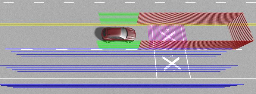
2 Wang et al.
sensor module illumination module
Powell lens
line sensor galvo galvo laser
line camera line laser lens collimation lens
(a) Working principle (b) Optical schematic (top view)
blind spot lane monitoring
lane marking
side-lane monitoring
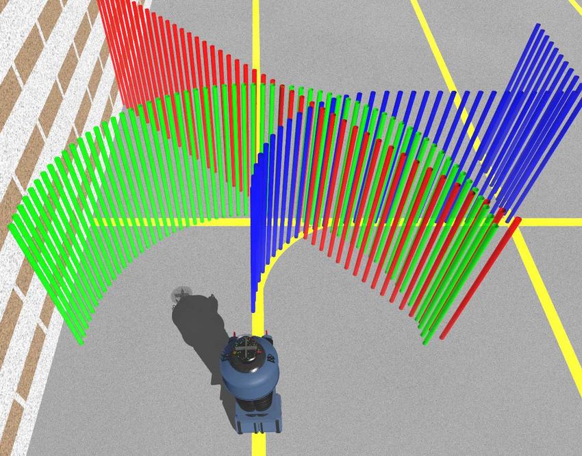
(c) Light curtains in a robot (d) Light curtains in a car
Fig. 1. We introduce the concept of a programmable triangulation light curtain — a
safety device that monitors object presence in a virtual shell around the device. (a,
b) This is implemented by intersecting a light plane emitted from a line laser and a
plane imaged by a line scan camera. The two planes are rapidly rotated in synchrony to
generate light curtains of varying shapes as demanded by the specifics of an application.
(c, d) Example curtains are shown for use on a robot and a car. The device detects
objects on the virtual curtains with little computational overhead, making it useful for
collision detection and avoidance.
We implement light curtains by triangulating an illumination plane, created
by fanning out a laser, with a sensing plane of a line sensor (see Fig. 1(a)).
In the absence of ambient illumination, the camera senses light only from the
intersection between these two planes — which is a line in the physical world. The
light curtain is then created by sweeping the illumination and sensing planes in
synchrony. This idea can be interpreted as a generalization of pushbroom stereo
[6] to active illumination for determining the presence of an object that intersects
an arbitrary ruled surface in 3D.
Benefits of triangulation light curtains. (1) Shape programmability: The
shape of a light curtain is programmable and can be configured dynamically
to suit the demands of the immediate task. For example, light curtains can be
used to determine whether a neighboring vehicle is changing lanes, whether a
pedestrian is in the crosswalk, or whether there are vehicles in adjacent lanes.
Similarly, a robot might use a curtain that extrudes its planned (even curved)
motion trajectory. Fig. 1(c, d) shows various light curtains for use in robots and
cars.
(2) Adaptability of power and exposure: Given an energy budget, in terms of
average laser power, exposure time, and refresh rate of the light curtain, we can
allocate higher power and exposure to lines in the curtain that are further away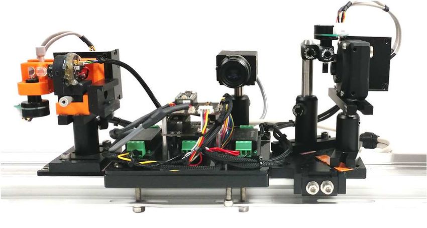
Programmable Triangulation Light Curtains          3

to combat inverse-square light fall-off. This is a significant advantage over tradi-
tional depth sensors that typically expend the same high power in all directions
to capture a 3D point cloud of the entire volume.
(3) Performance in scattering media: The optical design of the light curtain
shares similarities with confocal imaging [16] in that we selectively illuminate
and sense a small region. When imaging in scattering media, such as fog and
murky waters, this has the implicit advantage that back scattered photons are
optically avoided, thereby providing images with increased contrast.
(4) Performance in ambient light: A key advantage of programmable light cur-
tains is that we can concentrate the illumination and sensing to a thin region.
Together with the power and exposure adaptability, this enables significantly
better performance under strong ambient illumination, including direct sunlight,
at large distances (∼20-30m). The performance increases under cloudy skies and
indoors to 40m and 50m respectively.
(5) Dynamic range of the sensor: At any time instant, the sensor only captures
a single line of the light curtain that often has small depth variations and conse-
quently, little variation in intensity fall-off. Thus, the dynamic range of the mea-
sured brightness is often low. Hence, even a one-bit sensor with a programmable
threshold would be ample for the envisioned tasks.
(6) Sensor types: Any line sensor could be used with our design including inten-
sity sensors (CMOS, CCD, InGaAs [12]), time-of-flight (ToF) sensors (correla-
tion, SPAD [8]), and neuromorphic sensors (DVS) [15].
Limitations of triangulation light curtains. (1) Line-of-sight to the light
curtain. Our technique requires that the laser and sensor have line-of-sight to
the light curtain. When this is not the case, the intersection of line camera plane
and laser sheet is inside the object and is not seen by the camera; so the technique
will fail to detect objects intersecting with the light curtain. This can be resolved
partially by determining if there is an object between the system and the desired
curtain using a curtain whose “shape” is a sparse set of lines. (2) Interference:
When simultaneously used, several devices can accidentally interfere with each
other. This can be alleviated by using a time-of-flight sensor with different light
amplitude frequencies or adding a second line camera or several line lasers as
further discussed in the supplementary material. (3) Fast motion: Objects that
move at high speeds might be able to avoid detection by crossing the light curtain
in a region between two successive scans. However, the target would need to be
highly maneuverable to accomplish this given our high scan rate.

2   Related Work
Safety devices and proximity sensors. Devices such as “light curtains” [1], pressure-
sensitive mats, and conductive rubber edges are common safeguards used in
homes and factories. They are designed to stop the operation of a machine (e.g.
a garage door) automatically upon detection of a nearby object. Such proxim-
ity sensing devices use many physical modalities to detect presence including
capacitance, inductance, magnetism, infrared, ultrasound, Radar and LIDAR.
4      Wang et al.

Depth gating. Temporal gating [5, 10] uses a combination of a pulsed laser and
a camera with gated shutter, typically in the range of pico- to nano-seconds. By
delaying the exposure of the camera with respect to the laser pulse, the device
enables depth selection. An alternate approach relies on on-chip implementations
of temporal modulated light sources and sensors [22]. Our technique can be in-
terpreted as a specialized instance of primal-dual coding [20] where simultaneous
coding is performed at the camera and projector to probe the light transport
matrix associated with a scene, including implementing depth gating.
    The proposed technique is inspired from existing work on robust depth scan-
ning in presence of global and ambient light. Early work on imaging through
turbid includes scanning confocal microscopy [16] and light sheet microscopy
[25] which both illuminate and image the same depth with very shallow depth
of focus and block out-of-focus light i.e. scattered light during image formation.
Recent work for 3D measuring in scattering media have line striping-based [18]
and SPAD-based [21] methods through analyzing spatial or temporal distribu-
tion of photons, respectively. An effective method for handling ambient light is
concentrating the active light source’s output and scanning. Gupta et al. [11]
adjust the light concentration level in a structured light system adaptively ac-
cording to the ambient light level. Episcan3D [19] and EpiToF [3] scan a line
laser and a line sensor in synchrony such that the illumination and the sensing
planes are coplanar. Finally, there are many benefits in using special function-
ality sensors for imaging and depth scanning; examples include the DVS sensor
for structured light point scanning at high speed and dynamic range [17] as well
as the short-wave infrared sensor for enhanced eye-safe property and decreased
scattering [26, 24]. Such sensors can be easily incorporated in our light curtains
for additional robustness and capabilities.

3   Geometry of Triangulation Light Curtains

The proposed device consists of a line scan camera and a line scan laser, as
shown in Fig. 1(a, b). A Powell lens fans a laser beam out into a planar sheet
of light and the line camera senses light from a single plane. In the general
configuration, the two planes intersect at a line in 3D and, in the absence of
ambient and indirect illuminations, the sensor measures light scattered by any
object on the line. By rotating both the camera and the laser at a high speed,
we can sweep the intersecting line to form any ruled surface [2]. We refer to
this ruled surface, on which we detect presence of objects, as the light curtain.
The resulting device is programmable, in terms of its light curtain shape, and
flexible, in terms of being able to vary laser power and camera exposure time to
suit the demands of an application. In this section, we present the mathematical
model for a light curtain as a function of the camera and laser rotation axes.
Then, we describe how to estimate the camera and laser rotation angles for a
particular light curtain shape and show several examples.
    We consider the case where the camera and laser can each be rotated about a
single fixed parallel axis (see Fig. 2). This can be easily implemented by placing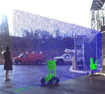
Programmable Triangulation Light Curtains 5
laser thickness
z
intersecting line
r curtain thickness
r x
ݎ ݎ
p(t) r
ݖ
ܾ ߜ
ߠ ߠ
camera laser camera ܾ laser
(a) Parallel rotation axis (b) Coordinate system (c) Top view
Fig. 2. (a) Viewing and illumination geometry of a triangulation light curtain generated
by rotating the laser light plane and sensor plane about parallel axes r. The intersection
line is also parallel to the two rotation axes. (b, c) The coordinate frame and top view
showing various parameters of interest. Note that changing θc and θp in synchrony
generates light curtains with different shapes. (c) The finite sizes of camera pixels and
finite thickness of laser sheet leads to a thick light curtain upon triangulation.
two 1D galvo mirrors, one each in the front of the line sensor and the laser,
respectively. Let the camera and laser rotation axes be r. We observe that inter-
secting line in the curtain will also be parallel and of the form
p0 + ur,
where p0 is any 3D point on the line and u ∈ (−α, α) is the offset along the axis
of rotation (see Fig. 2(a, b)). Then, the light curtain s(t, u) ⊂ R3 is obtained by
sweeping the intersection line such that
s(t, u) = p(t) + ur,
where p(t) ∈ R3 is a 3D path that describes the points scanned by the center
pixel on the line sensor and t ∈ [0, 1] is the parameterization of the path.
Given a light curtain s(t, u), we next show how to compute the rotation angles
of the camera and laser respectively. Without loss of generality, we assume that
the origin of our coordinate system is at the midpoint between the centers of the
line camera and the laser. We further assume that the rotation axes are aligned
along the y-axis and that the 3D path can be written as p(t) = [x(t), 0, z(t)]⊤ .
To achieve this light curtain, suppose that the laser rotates about its axis with
an angular profile of θp (t), where the angle is measured counter-clockwise with
respect to the x-axis. Similarly, the line sensor rotates with an angular profile of
θc (t). Let b be the baseline between the laser and the line camera. We can derive
θc (t) and θp (t) as
θc (t) atan2(z(t), x(t) + b/2)
= . (1)
θp (t) atan2(z(t), x(t) − b/2)
Fig. 1(c, d) shows different types of light curtains for use on robots and cars
and Fig. 3 explains each in detail. For each curtain, we show the rendered scene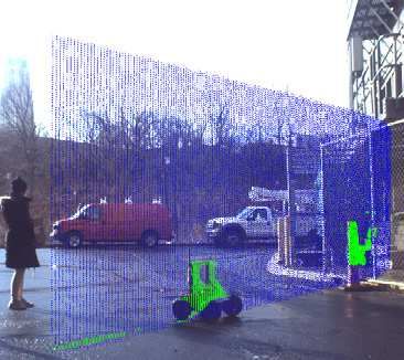
6 Wang et al.
Relative
Cylindrical safety curtain Z-axis Unit: degrees Unit: m Light fall-off exposure/power
camera ߠ
laser ߠ
start end
Planning path curtain X-axis ݐ ݐ ݐ
Lane curtain
Blind spot zone curtain
Discrete road sampling
Lane marking observer
(a) Application scenarios (b) 2D cross section (c) ߠ ሺݐሻ and ߠ ሺݐሻ (d) Uncertainty U (e) Light fall-off
Fig. 3. Different types of light curtains used by a robot and a car. (a) Envisioned
application scenarios visualized using 3D renderings. (b) 2D cross section (all units in
meters) of the light curtain and placement of the camera and laser (baselines in the
first two rows was 300mm, third row was 2m, and the remaining rows was 200mm).
The arrow on the curtain indicates the scanning direction. (c) Rotation angle profiles
of camera and laser to achieve desired light curtain in each scan. (d) Thickness of the
light curtain for a camera with 50µm pixel width and focal length 6mm. (e) Light
fall-off and the corresponding adaptation of exposure/power to compensate for it.
with the light curtain, a 2D cross section of the curtain, and the corresponding
rotation angle profiles θc (t) and θp (t), computed using (1). The first two light
curtains — a cylindrical curtain for safety zone monitoring and a curved curtain
for monitoring obstacles along a path — are envisioned for use on robots. The
next four kinds of curtains are envisioned for use on cars: ⊓-shape lane curtain
to detect proximity vehicles in front as well as those that encroach on to the lane
being used (row 3), side curtain to cover blind spot zones (row 4), and a discrete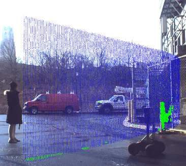
Programmable Triangulation Light Curtains        7

sampling of neighbor lane’s condition to identify presence of a vehicle in that
volume (row 5). As noted in the introduction, light curtains also offer improved
contrast in the presence of scattering media and hence, a curtain observing lane
markings (row 6) is especially useful on foggy days.
    Our proposed device can also be configured with the line sensor and laser
rotating over non-parallel axes or even with each of them enjoying full rota-
tional degree of freedom. These configurations can generate other kinds of ruled
surfaces including, for example, a Möbius strip. We leave the discussion to the
supplementary material. For applications that require light curtains of arbitrary
shapes, we would need to use point sources and detectors; this, however, comes
at the cost of large acquisition time that is required for two degrees of freedom
in scanning. On the other hand, 2D imaging with a divergent source does not re-
quire any scanning but has poor energy efficiency and flexibility. In comparison,
line sensors and line lasers provide a unique operating point with high acquisition
speeds, high energy efficiency, and a wide range of light curtain shapes.

4   Optimizing Triangulation Light Curtains
We now quantify parameters of interest in practical light curtains — for example
their thickness and signal-to-noise ratio (SNR) of measured detections — and
approaches to optimize them. In particular, we are interested in minimizing
thickness of the curtain as well as optimizing exposure time and laser power for
improved detection accuracy when the curtain spans a large range of depths.

Thickness of light curtain. The light curtain produced by our device has a finite
thickness due to the finite sizes of the sensor pixels and the laser illumination.
Suppose that the laser plane has a thickness of ∆L meters and each pixel has an
angular extent of δc radians. Given a device with a baseline of length b meters
and imaging a point at depth z(t) = z, the thickness of the light curtain is given
as an area of a parallelogram shaded in Fig. 2(c), which evaluates to

                                      rc2 rp δc ∆L
                                 A=                                            (2)
                                        z       b
where rc and rp is the distance between the intersected point and the camera
and laser, respectively. We provide the derivation in the supplemental material.
Finally, given that different light curtain geometries can produce curtains of
the same area, a more intuitive and meaningful metric for characterizing the
thickness is the length
                                     A      r 2 rp δ c
                               U=        = c           .                       (3)
                                    ∆L        z b
    In any given system, changing the laser thickness ∆L requires changing the
optics of the illumination module. Similarly, changing δc requires either chang-
ing the pixel width or the focal length of the camera. In contrast, varying the
baseline provides an easier alternative to changing the thickness of the curtain
that involves a single translation. This is important since different applications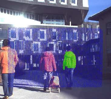
8       Wang et al.

often have differing needs on the thickness of the curtain. A larger baseline helps
in achieving very thin curtains which is important when there is a critical need
to avoid false alarm. On the other hand, thick curtains that can be achieved
by having a smaller baseline are important in scenarios where mis-detections,
especially those arising from the discreteness of the curtain, are to be avoided.
    In Fig. 3(d), we visualize the thickness of various light curtains. We set the
camera’s pixel width to 50µm with a lens of focal length f = 6mm, thereby
giving us a value for δc = 50µm f   = 0.008 radians. The baseline b was set to
300mm for the first two rows, 2m for the third row, and 200mm for the last
three rows. For example, for the lane marking observer (last row), a thickness of
2m at the furthest point is beneficial to deal with uneven roads.

Adapting laser power and exposure. Another key advantage of our light curtain
device is that we can adapt the power of the laser or the exposure time for
each intersecting line to compensate for light fall-off, which is inversely propor-
tional to the square of the depth. In a traditional projector-camera system, it is
common to increase the brightness of the projection to compensate for light fall-
off, so that far-away scenes points can be well illuminated; however, this would
imply that points close to the camera get saturated easily thereby requiring a
high dynamic range camera. In contrast, our system has an additional degree of
freedom where-in the laser’s power and/or the camera’s exposure time can be
adjusted according to depth so that light fall-off is compensated to the extent
possible under the device constraints and eye safety. Further, because our device
only detects presence or absence of objects, in an ideal scenario where albedo is
the same everywhere, the laser can send small amounts of light to just overcome
the camera’s readout noise or the photon noise of ambient light, and only a 1-bit
camera is required. Fig. 3(e) shows light fall-off and depth-adaptive exposure
time or laser power for all the light curtains.

Combining with time-of-flight sensors. The analysis in (3) indicates that U ≈
z 2 δc
   b   when rc , rp ≈ z and light curtain is expected to get thicker, quadratically,
with depth. Increasing baseline and other parameters of the system can only
alleviate this effect in part due to the physical constraints on sensor size, laser
spot thickness as well as the baseline. We show that replacing the line intensity
sensor with a 1D continuous-wave time-of-flight (CW-TOF) sensor [14] alleviates
the quadratic dependence of thickness with depth.
      CW-TOF sensors measure phase to obtain depth. A CW-TOF sensor works
by illuminating the scene with an amplitude modulated wave, typically a peri-
odic signal of frequency fm Hz, and measuring the phase difference between the
illumination and the light received at each pixel. The phase difference φ and the
depth d of the scene point are related as

                              φ = mod (fm d/c, 2π) .

As a consequence, the depth resolution of a TOF sensor ∆d = c∆φfm (ignoring
the phase wrapping) is constant and independent of depth. Further, the depth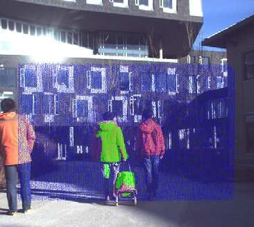
Programmable Triangulation Light Curtains        9

resolution increases with the frequency of the amplitude wave. However, TOF-
based depth recovery has a phase wrapping problem due to the presence of the
mod(·) operator; this implies that the depth estimate has an ambiguity prob-
lem and this problem gets worse at higher frequencies. In contrast, traditional
triangulation-based depth estimation has no ambiguity problem, but at the cost
of quadratic depth uncertainty.
    We can leverage the complementary strengths of traditional triangulation
and CW-TOF to enable light curtains with near-constant thickness over a large
range. This is achieved as follows. First, the phase and intensity of the trian-
gulated region are measured by the CW-TOF sensor; examples of this is shown
in Fig. 8(iii, iv). Second, knowing the depth of the curtain, we can calculate
the appropriate phase to retain and discard pixels with phase values that are
significantly different. An alternative approach to achieving this is to perform
phase-based depth gating using appropriate codes at illumination and sensing
[22]. The use of triangulation automatically eliminates the depth ambiguity of
phase-based gating provided the thickness of the triangulation is smaller than
half of the wavelength of the amplitude wave. With this, it is possible to create
thinner light curtains over a larger depth range.

5   Hardware Prototype

Our prototype device has two modules (see Fig. 4). At the sensor end, we use
an Alkeria NECTA N2K2-7 line intensity sensor with a 6mm f /2 S-mount lens
whose diagonal FOV is 45◦ and image circle has a diameter of 7mm. The line
camera has 2048 × 2 pixels with pixel size 7µm × 7µm; we only use the central
1000 × 2 pixels due to the lens’ limited circle of illumination. The line sensor is
capable of reading out 95, 057 lines/second. We fit it with an optical bandpass
filter, 630nm center wavelength and 50nm bandwidth to suppress ambient light.
For the ToF prototype, we used a Hamamatsu S11961-01CR sensor in place of
the intensity sensor whose pixel size is 20µm×50µm. We used a low cost 1D galvo
mirror to rotate the camera’s viewing angle. The 2D helper FLIR camera (shown
in the middle) is used for one-time calibration of the device and visualizing the
light curtains in the scene of interest by projecting the curtain to its view.
     At the illumination side, we used a Thorlabs L638P700M 638nm laser diode
with peak power of 700mW . The laser is collimated and then stretched into a
line with a 45◦ Powell lens. As with the sensor side, we used a 1D galvo mirror
to steer the laser sheet. The galvo mirror has dimension of 11mm × 7mm, and
has 22.5◦ mechanical angle and can give the camera and laser 45◦ FOV since
optical angle is twice the mechanical angle. It needs 500µs to rotate 0.2◦ optical
angle. A micro-controller (Teensy 3.2) is used to synchronize the camera, the
laser and the galvos. Finally, we aligned the rotation axes to be parallel and
fixed the baseline as 300mm. The FOV is approximately 45◦ × 45◦ .

Ambient light. The camera also measures the contribution from the ambient
light illuminating the entire scene. To suppress this, we capture two images at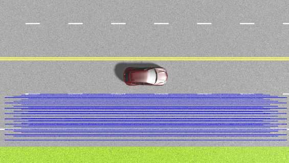
10       Wang et al.

                                                                   Laser
                                                              A    Thorlabs L638P700M
                                                                   Powell lens
                                   G            E D           B
     B    A                                                        Thorlabs PL0145
 C                                          F                      Galvo mirror
                                                              C    Wonsung P/N 0738770883980
                                                                   Line sensor
                                                              D    Alkeria NECTA N2K2-7
                                                                   Lens for line sensor
                                                              E    Boowon BW60BLF
                                                                   Galvo mirror
                                                               F
                                                                   Same as C
                                                                   2D helper camera
                                                              G    FLIR GS3-U3-23S6C-C
                                                                   (for calibration only)

Fig. 4. Hardware prototype with components marked. The prototype implements the
schematic shown in Fig. 1(b).

each setting of the galvos — one with and one without the laser illumination,
each with exposure of 100µs. Subtracting the two suppresses the ambient image.

Scan rate. Our prototype is implemented with galvo mirrors that take about
500 µs to stabilize, which limits the overall frame-rate of the device. Adding
two 100µs exposures for laser on and off, respectively, allows us to display 1400
lines per second. In our experiments, we design the curtains with 200 lines, and
we sweep the entire curtain at a refresh rate of 5.6 fps. To increase the refresh
rate, we can use higher-quality galvo mirrors with lower settling time, a 2D
rolling shutter camera as in [19] or spatially-multiplexed line camera by digital
micromirror device (DMD) [23] in the imaging side and a MEMS mirror on the
laser side so that 30 fps can be easily reached.

Calibration and eye safety. Successful and safe deployment of light curtains re-
quire precise calibration as well as specifications of laser eye safety. Calibration
is done by identifying the plane in the real world associated with each setting
of laser’s galvo and the line associated with each pair of camera’s galvo and
camera’s pixel. We use a helper camera and projector to perform calibration,
following steps largely adapted from prior work in calibration [7, 13]. The sup-
plemental material has detailed explanation for both calibration and laser eye
safety calculations based on standards [4].

6    Results
Evaluating programmability of triangulation light curtains. Fig. 5 shows the re-
sults of implementing various light curtain shapes both indoors and outdoors.
When nothing “touches” the light curtain, the image is dark; when a person or
other intruders touch the light curtain, it is immediately detected. The small
insets show the actual images captured by the line sensor (after ambient sub-
traction) mosaicked for visualization. The light curtain and the detection are
Programmable Triangulation Light Curtains 11
6
6 5
4
4 3
2
2 1
0
0 2
0
-2 0 2 -2 -1 0 1 2
y x
x
6
6
4
4
2
2
0
2
0
0
-2 0
-2 0 2 y
x x
6
6
5
4
4
3
2
2 1
0
2
0 0
-2 0 2 -2
0 1 2
x y x
6
6
4 4
2
2
0
2
0 0 2
-2 0 2 -2 0
1
y -1
x x
156
15
5
104
10
3
52
5 1
0
5 52
0 0
-2-5
-5 0 5 0
y x
x
6
5
4
4 3
2
2 1
0
2
0 0 1
-2 0 2 0
-2 -1
x y x
Fig. 5. Generating light curtains with different shapes. The images shown are from
the 2D helper camera’s view with the light curtain rendered in blue and detections
rendered in green. The curtains are shown both indoors and outdoors in sunlight. The
insets are images captured by the line sensor as people/objects intersect the curtains.
The curtains have 200 lines with a refresh rate of 5.6 fps. The curtain in the second
row detects objects by sampling a volume with a discrete set of lines.
geometrically mapped to the 2D helper camera’s view for visualization. Our
prototype uses a visible spectrum (red) laser and switching to near infrared can
improve performance when the visible albedo is low (e.g. dark clothing).
Light curtains under sunlight. Fig. 6(a) shows the detections of a white board
placed at different depths (verified using a laser range finder) in bright sunlight
(∼ 100klx). The ambient light suppression is good even at 25m range. Under12 Wang et al.
16
12
8
4
2D
0
scene at 5m at 15m at 25m at 35m
(b) Depth map by
(a) Fronto-parallel planar light curtain at different depths sweeping light curtains
Fig. 6. Performance under bright sunlight (100klux) for two different scenes. (a) We
show raw light curtain data, without post-processing, at various depths from a white
board. Notice the small speck of the board visible even at 35m. (b) We sweep the light
curtain over the entire scene to generate a depth map.
2D camera
Light Curtain
Fig. 7. Seeing through volumetric scattering media. Light curtains suppress backscat-
tered light and provide images with improved contrast.
cloudy skies, the range increases to more than 40m. Indoors, the range is approx-
imately 50m. These ranges assume the same refresh rate (and exposure time)
for the curtains. In Fig. 6(b), we verify the accuracy of the planar curtains by
sweeping a fronto-parallel curtain over a dense set of depths and visualizing the
resulting detections as a depth map.
Performance under volumetric scattering. When imaging in scattering media,
light curtains provide images with higher contrast by suppressing backscattered
light from the medium. This can be observed in Fig. 7 where we show images of
an outdoor road sign under heavy smoke from a planar light curtain as well as a
conventional 2D camera. The 2D camera provides images with low contrast due
to volumetric scattering of the sunlight, the ambient source in the scene.
Reducing curtain thickness using a TOF sensor. We use our device with a line
TOF sensor to form a fronto-parallel light curtain at a fixed depth. The results
are shown in Fig. 8. Because of triangulation uncertainty, the camera could see
a wide depth range as shown in (a.iii) and (b.iii). However, phase data, (a.iv)Programmable Triangulation Light Curtains 13
1
0.8
0.6
0.4
0.2
0
(i) scene (ii) light curtain (iii) triangulation (iv) phase w/o (v) phase +
with thickness wrapping triangulation
(a) Staircase scene
1
0.8
0.6
0.4
0.2
0
(i) scene (ii) light curtain (iii) triangulation (iv) phase with (v) Phase +
with thickness wrapping triangulation
(b) Lab scene
Fig. 8. Using line CW-TOF sensor. For both scenes, we show that fusing (iii) trian-
gulation gating with (iv) phase information leads to (v) thinner light curtains without
any phase wrapping ambiguity.
and (b.iv) helps to decrease the uncertainty as shown in (a.v) and (b.v). Note
that in (b.iv), there is phase wrapping which is mitigated using triangulation.
Adapting laser power and exposure. Finally, we showcase the flexibility of our
device in combating light fall-off by adapting the exposure and/or the power of
the laser associated with each line in the curtain. We show this using depth maps
sensed by sweeping fronto-parallel curtains with various depth settings. For each
pixel we assign the depth value of the planar curtain at which its intensity value
is the highest. We use an intensity map to save this highest intensity value. In
Fig. 9(a), we sweep 120 depth planes in an indoor scene. We performed three
strategies: two constant exposures per intersecting line and one that is depth-
adaptive such that exposure is linear in depth. We show intensity map and depth
map for each strategy. Notice the saturation and darkness in intensity maps with
the constant exposure strategies and even brightness with the adaptive strategy.
The performance of the depth-adaptive exposure is similar to that of a constant
exposure mode whose total exposure time is twice as much. Fig. 9(b) shows
a result on an outdoor scene with curtains at 40 depths, but here the power
is adapted linearly with depth. As before, a depth-adaptive budgeting of laser
power produces depth maps that are similar to those of a constant power mode
with 2× the total power. Strictly speaking, depth-adaptive budgeting should be
quadratic though we use a linear approximation for ease of comparison.14 Wang et al.
ᬅ ᬅ ᬆ ᬇ
depth
ᬇ ᬆ
exposure
(a) Constant exposure time vs. depth-adaptive exposure time
ᬅ ᬅ ᬆ ᬇ 12
depth
8
ᬇ ᬆ
4
power 0
(b) Constant power vs. depth-adaptive power
Fig. 9. We use depth adaptive budgeting of (a) exposure and (b) power to construct
high-quality depth maps by sweeping a fronto-parallel curtain. In each case, we show
the results of three strategies: (1) constant exposure/power at a low value, (2) constant
exposure/power at a high value, and (3) depth-adaptive allocation of exposure/power
such that the average matches the value used in (1). We observe that (3) achieves the
same quality of depth map as (2), but using the same time/power budget as in (1).
7 Discussion
A 3D sensor like LIDAR is often used for road scene understanding today. Let
us briefly see how it is used. The large captured point cloud is registered to a
pre-built or accumulated 3D map with or without the help of GPS and IMU.
Then, dynamic obstacles are detected, segmented, classified using complex, com-
putationally heavy and memory intensive deep learning approaches [9, 27]. These
approaches are proving to be more and more successful but perhaps all this com-
putational machinery is not required to answer questions, such as: “Is an object
cutting across into my lane?”, or “Is an object in a cross-walk?”.
This paper shows that our programmable triangulation light curtain can pro-
vide an alternative solution that needs little to no computational overhead, and
yet has high energy efficiency and flexibility. We are by no means claiming that
full 3D sensors are not useful but are asserting that light curtains are an effec-
tive addition when depths can be pre-specified. Given its inherent advantages, we
believe that light curtains will be of immense use in autonomous cars, robotics
safety applications and human-robot collaborative manufacturing.
Acknowledgments
This research was supported in parts by an ONR grant N00014-15-1-2358, an
ONR DURIP Award N00014-16-1-2906, and DARPA REVEAL Co-operative
Agreement HR0011-16-2-0021. A. C. Sankaranarayanan was supported in part
by the NSF CAREER grant CCF-1652569. J. Bartels was supported by NASA
fellowship NNX14AM53H.Programmable Triangulation Light Curtains 15
References
1. Light curtain wikipedia. https://en.wikipedia.org/wiki/Light curtain
2. Ruled surface wikipedia. https://en.wikipedia.org/wiki/Ruled surface
3. Achar, S., Bartels, J.R., Whittaker, W.L., Kutulakos, K.N., Narasimhan, S.G.:
Epipolar time-of-flight imaging. ACM Transactions on Graphics (TOG) 36(4), 37
(2017)
4. American National Standards Institute: American national standard for safe use
of lasers z136.1 (2014)
5. Baker, I.M., Duncan, S.S., Copley, J.W.: A low-noise laser-gated imaging system
for long-range target identification. In: Defense and Security. pp. 133–144. Inter-
national Society for Optics and Photonics (2004)
6. Barry, A.J., Tedrake, R.: Pushbroom stereo for high-speed navigation in cluttered
environments. In: International Conference on Robotics and Automation (ICRA).
pp. 3046–3052. IEEE (2015)
7. Bouguet, J.Y.: Matlab camera calibration toolbox.
http://www.vision.caltech.edu/bouguetj/calib doc/ (2000)
8. Burri, S., Homulle, H., Bruschini, C., Charbon, E.: Linospad: a time-resolved 256×
1 cmos spad line sensor system featuring 64 fpga-based tdc channels running at up
to 8.5 giga-events per second. In: Optical Sensing and Detection IV. vol. 9899, p.
98990D. International Society for Optics and Photonics (2016)
9. Geiger, A., Lenz, P., Urtasun, R.: Are we ready for autonomous driving? the kitti
vision benchmark suite. In: Conference on Computer Vision and Pattern Recogni-
tion (CVPR). pp. 3354–3361. IEEE (2012)
10. Grauer, Y., Sonn, E.: Active gated imaging for automotive safety applications. In:
Video Surveillance and Transportation Imaging Applications 2015. vol. 9407, p.
94070F. International Society for Optics and Photonics (2015)
11. Gupta, M., Yin, Q., Nayar, S.K.: Structured light in sunlight. In: International
Conference on Computer Vision (ICCV). pp. 545–552. IEEE (2013)
12. Hansen, M.P., Malchow, D.S.: Overview of swir detectors, cameras, and applica-
tions. In: Thermosense Xxx. vol. 6939, p. 69390I. International Society for Optics
and Photonics (2008)
13. Lanman, D., Taubin, G.: Build your own 3d scanner: 3d photography for beginners.
In: ACM SIGGRAPH 2009 Courses. p. 8. ACM (2009)
14. Li, L.: Time-of-flight camera–an introduction. Technical white paper (SLOA190B)
(2014)
15. Lichtsteiner, P., Posch, C., Delbruck, T.: A 128x128 120 dB 15us latency asyn-
chronous temporal contrast vision sensor. IEEE journal of solid state circuits 43(2),
566–576 (2008)
16. Marvin, M.: Microscopy apparatus (Dec 19 1961), US Patent 3,013,467
17. Matsuda, N., Cossairt, O., Gupta, M.: Mc3d: Motion contrast 3d scanning. In:
International Conference on Computational Photography (ICCP). pp. 1–10. IEEE
(2015)
18. Narasimhan, S.G., Nayar, S.K., Sun, B., Koppal, S.J.: Structured light in scattering
media. In: International Conference on Computer Vision (ICCV). vol. 1, pp. 420–
427. IEEE (2005)
19. O’Toole, M., Achar, S., Narasimhan, S.G., Kutulakos, K.N.: Homogeneous codes
for energy-efficient illumination and imaging. ACM Transactions on Graphics
(ToG) 34(4), 35 (2015)16 Wang et al.
20. O’Toole, M., Raskar, R., Kutulakos, K.N.: Primal-dual coding to probe light trans-
port. ACM Transactions on Graphics (ToG) 31(4), 39–1 (2012)
21. Satat, G., Tancik, M., Raskar, R.: Towards photography through realistic fog. In:
International Conference on Computational Photography (ICCP). pp. 1–10. IEEE
(2018)
22. Tadano, R., Kumar Pediredla, A., Veeraraghavan, A.: Depth selective camera: A
direct, on-chip, programmable technique for depth selectivity in photography. In:
International Conference on Computer Vision (ICCV). pp. 3595–3603. IEEE (2015)
23. Wang, J., Gupta, M., Sankaranarayanan, A.C.: Lisens-a scalable architecture for
video compressive sensing. In: International Conference on Computational Pho-
tography (ICCP). IEEE (2015)
24. Wang, J., Sankaranarayanan, A.C., Gupta, M., Narasimhan, S.G.: Dual structured
light 3d using a 1d sensor. In: European Conference on Computer Vision (ECCV).
pp. 383–398. Springer (2016)
25. Weber, M., Mickoleit, M., Huisken, J.: Light sheet microscopy. In: Methods in cell
biology, vol. 123, pp. 193–215. Elsevier (2014)
26. Wheaton, S., Bonakdar, A., Nia, I.H., Tan, C.L., Fathipour, V., Mohseni, H.:
Open architecture time of fight 3d swir camera operating at 150 mhz modulation
frequency. Optics Express 25(16), 19291–19297 (2017)
27. Zhou, Y., Tuzel, O.: Voxelnet: End-to-end learning for point cloud based 3d ob-
ject detection. Conference on Computer Vision and Pattern Recognition (CVPR)
(2018)You can also read