Blur Aware Calibration of Multi-Focus Plenoptic Camera
←
→
Page content transcription
If your browser does not render page correctly, please read the page content below
This paper has been accepted for publication at the
IEEE Conference on Computer Vision and Pattern Recognition (CVPR), Seattle, 2020. c IEEE
Blur Aware Calibration of Multi-Focus Plenoptic Camera
Mathieu Labussière1 , Céline Teulière1 , Frédéric Bernardin2 , Omar Ait-Aider1
1
Université Clermont Auvergne, CNRS, SIGMA Clermont,
Institut Pascal, F-63000 Clermont-Ferrand, France
2
Cerema, Équipe-projet STI, 10 rue Bernard Palissy, F-63017 Clermont-Ferrand, France
mathieu.labu@gmail.com, firstname.name@{uca,cerema}.fr
arXiv:2004.07745v1 [eess.IV] 16 Apr 2020
Abstract
This paper presents a novel calibration algorithm for
Multi-Focus Plenoptic Cameras (MFPCs) using raw im-
ages only. The design of such cameras is usually complex
and relies on precise placement of optic elements. Several
calibration procedures have been proposed to retrieve the
camera parameters but relying on simplified models, recon-
structed images to extract features, or multiple calibrations
when several types of micro-lens are used. Considering
blur information, we propose a new Blur Aware Plenop-
tic (BAP) feature. It is first exploited in a pre-calibration
step that retrieves initial camera parameters, and secondly
to express a new cost function for our single optimization
process. The effectiveness of our calibration method is val-
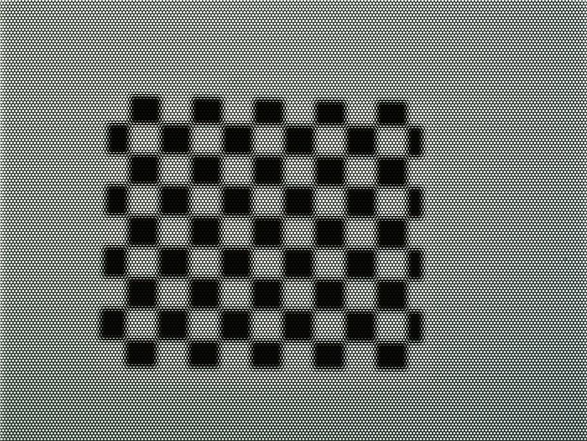
Figure 1: The Raytrix R12 multi-focus plenoptic cam-
idated by quantitative and qualitative experiments.
era used in our experimental setup (a), along with a raw
image of a checkerboard calibration target (b). The image
is composed of several micro-images with different blurred
1. Introduction
levels and arranged in an hexagonal grid. In each micro-
The purpose of an imaging system is to map incoming image, our new Blur Aware Plenoptic (BAP) feature is il-
light rays from the scene onto pixels of photo-sensitive de- lustrated by its center and its blur radius (c).
tector. The radiance of a light ray is given by the plenop-
tic function L (x, θ, λ, τ ), introduced by Adelson et al. [1], The mapping of incoming light rays from the scene onto
where x ∈ R3 is the spatial position of observation, θ ∈ R2 pixels can be expressed as a function of the camera model.
is the angular direction of observation, λ is the wavelength Classical cameras are usually modeled as pinhole or thin
of the light and τ is the time. Conventional cameras capture lens. Due to the complexity of plenoptic camera’s design,
only one point of view. A plenoptic camera is a device that the used models are usually high dimensional. Specific cal-
allows to retrieve spatial as well as angular information. ibration methods have to be developed to retrieve the intrin-
sic parameters of these models.
From Lumigraph [17] to commercial plenoptic cameras
[19, 23], several designs have been proposed. This paper 1.1. Related Work
focuses on plenoptic cameras based on a Micro-Lenses Ar-
ray (MLA) placed between the main lens and the photo- Unfocused plenoptic camera calibration. In this config-
sensitive sensor (see Fig. 2). The specific design of such a uration, light rays are focused by the MLA on the sensor
camera allows to multiplex both types of information onto plane. The calibration of unfocused plenoptic camera [19]
the sensor in the form of a Micro-Images Array (MIA) (see has been widely studied in the literature [6, 2, 25, 24, 11,
Fig. 1 (b)), but implies a trade-off between the angular and 36]. Most approaches rely on a thin-lens model for the main
spatial resolutions [10, 16, 8]. It is balanced according to lens and an array of pinholes for the micro-lenses. Most of
the MLA position with respect to the main lens focal plane them require reconstructed images to extract features, and
(i.e., focused [23, 9] and unfocused [19] configurations). limit their model to the unfocused configuration, i.e., set-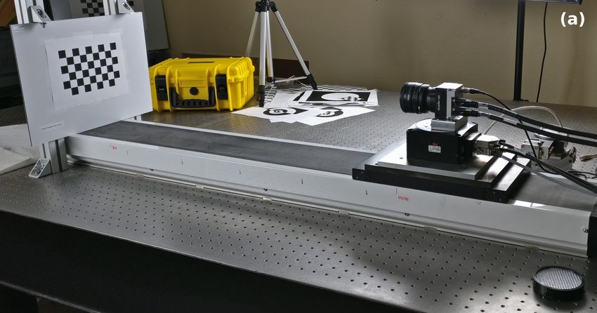
ting the micro-lens focal length at the distance MLA-sensor.               Sensor                                        xw zw
Therefore those models cannot be directly extended to the                              MLA                                  yw
focused or multi-focus plenoptic camera.                                 ∆c                                 Main Lens
                                                                                                                                  object

Focused plenoptic camera calibration. With the arrival                                                               A
of commercial focused plenoptic cameras [18, 23], new                                                            O
calibration methods have been proposed. Based on [14],                    (u0 , v0 )                 bl                          al
Heinze et al. [13] have developed a new projection model                                                                    //
                                                                  image            d             D
and a metric calibration procedure which is incorporated
in the RxLive software of Raytrix GmbH. Other cal-                                           F
ibration methods and models have been proposed, either                                                    ck,l
to overcome the fragility of the initialization [26], or to                                                          Ck,l
model more finely the camera parameters using depth in-                                                   ck,l
                                                                                                           0     f (i)
formation [33, 32]. O’Brien et al. [22] introduced a new                                         s                           ∆C
3D feature called plenoptic disc and defined by its center
                                                                  Figure 2: Focused Plenoptic Camera model in Galilean con-
and its radius. Nevertheless, all previous methods rely on
                                                                  figuration (i.e., the main lens focuses behind the sensor)
reconstructed images meaning that they introduce error in
                                                                  with the notations used in this paper.
the reconstruction step as well as in the calibration process.
    To overcome this problem, several calibration meth-           A visual overview of our method is given in Fig. 3. The
ods [35, 34, 29, 20, 3, 21, 31] have been proposed using          remainder of this paper is organized as follows: first, the
only raw plenoptic images. In particular, features extrac-        camera model and BAP feature are presented in Section 2.
tion in raw micro-images has been studied in [3, 21, 20]          The proposed pre-calibration step is explained in Section 3.
achieving improved performance through automation and             Then, the feature detection is detailed in Section 4 and the
accurate identification of feature correspondences. How-          calibration process in Section 5. Finally, our results are pre-
ever, most of the methods rely on simplified models for op-       sented and discussed in Section 6. The notations used in
tic elements: the MLA is modeled as a pinholes array mak-         this paper are shown in Fig. 2. Pixel counterparts of metric
ing it impossible to retrieve the focal lengths, or the MLA       values are denoted in lower-case Greek letters.
misalignment is not considered. Some do not consider dis-
tortions [35, 21, 31] or restrict themselves to the focused       2. Camera model and BAP feature
case [35, 34, 20].
    Finally, few have considered the multi-focus case [13, 3,     2.1. Multi-focus Plenoptic Camera
21, 31] but dealt with it in separate processes, leading to          We consider multi-focus plenoptic cameras as described
different intrinsic and extrinsic parameters according to the     in [9, 23]. The main lens, modeled as a thin-lens, maps
type of micro-lenses.                                             object point to virtual point behind (resp., in front of) the
1.2. Contributions                                                image sensor in Galilean (resp., Keplerian) configuration.
                                                                  Therefore, the MLA consists of I different lens types with
   This paper focuses on the calibration of micro-lenses-         focal lengths f (i) , i ∈ {1, . . . , I} which are focused on
based Multi-Focus Plenoptic Camera (MFPC). To the best            I different planes behind the image sensor. This multi-
of our knowledge, this is the first method proposing a sin-       focus setup corresponds to the Raytrix camera system
gle optimization process that retrieves intrinsic and extrinsic   described in [23] when I = 3. The micro-lenses are mod-
parameters of a MFPC directly from raw plenoptic images.          eled as thin-lenses allowing to take into account blur in the
The main contributions are the following:                         micro-image. Our model takes into account the MLA mis-
   • We present a new Blur Aware Plenoptic (BAP) feature          alignment, freeing all six degrees of freedom.
     defined in raw image space that enables us to handle            The tilt of the main lens is included in the distortion
     the multi-focus case.                                        model and we make the hypothesis that the main lens plane
   • We introduce a new pre-calibration step using BAP            Πl is parallel to the sensor plane Πs . Furthermore, we
     features from white images to provide a robust initial       choose the main lens frame as our camera reference frame,
     estimate of internal parameters.                             with O being the origin, the z-axis coinciding with the op-
   • We propose a new reprojection error function exploit-        tical axis and pointing outside the camera, and the y-axis
     ing BAP features to refine a more complete model, in-        pointing downwards. Only distortions of the main lens are
     cluding in particular the multiple micro-lenses focal        considered. We use the model of Brown-Conrady [4, 5]
     lengths. Our checkerboard-based calibration is con-          with three coefficients for the radial component and two for
     ducted in a single optimization process.                     the tangential.
Furthermore, we take into account the deviation of the we introduce a new Blur Aware Plenoptic (BAP) feature
image center and the optical center for each micro-lens be- characterized by its center and its radius, i.e., p = (u, v, ρ).
cause it tends to cause inaccuracy in decoded light field. Therefore, our complete plenoptic camera model allows
Therefore, the principal point ck,l
0 of the micro-lens indexed us to link a scene point pw to our new BAP feature p
by (k, l) is given by through each micro-lens (k, l)
uk,l u
d u0
ck,l
0 =
0 = − c k,l + ck,l , (1) v
v0k,l D+d v0 ∝ P (i, k, l) · Tµ (k, l) · ϕ(K(F ) · Tc · pw ) , (5)
ρ
where ck,l is the center in pixels of the micro-image (k, l), 1
>
u0 v0 is the main lens principal point, d is the distance
where P (i, k, l) is the blur aware plenoptic projection ma-
MLA-sensor and D is the distance main lens-MLA, as illus-
trix through the micro-lens (k, l) of type i, and computed
trated in Fig. 2.
as
Finally, each micro-lens produces a micro-image onto
the sensor. The set of these micro-images has the same P (i, k, l) = P (k, l) · K f (i) (6)
structural organization as the MLA, i.e., in our case an
uk,l
hexagonal grid, alternating between each type of micro- d/s 0 0 0 1 0 0 0
lens. The data can therefore be interpreted as an array of 0 d/s v k,l 0 0 1 0 0
= 0 .
∆C ∆C 0 0 1 0
micro-images, called by analogy the MIA. The MIA coor- 0 0 s 2 −s 2 d
dinates are expressed in image space. Let δc be the pixel dis- 0 0 −1 0 0 0 −1/f (i) 1
tance between two arbitrary consecutive micro-images cen-
ters ck,l . With s the metric size of a pixel, let ∆c = s · δc be P (k, l) is a matrix that projects the 3D point onto the sen-
its metric value, and ∆C be the metric distance between the sor. K(f ) is the thin-lens projection matrix for the given
two corresponding micro-lenses centers Ck,l . From similar focal length. Tc is the pose of the main lens with respect
triangles, the ratio between them is given by to the world frame and Tµ (k, l) is the pose of the micro-
lens (k, l) expressed in the camera frame. The function ϕ(·)
∆C D D models the lateral distortion.
= ⇐⇒ ∆C = ∆c · . (2)
∆c d+D d+D Finally, the projection model defined in Eq. (5) con-
sists of a set Ξ of (16 + I) intrinsic parameters to be opti-
We make the hypothesis that ∆C is equal to the micro-lens
mized, including the main lens focal length F and its 5 lat-
diameter. Since d
D, we can make the following ap-
eral distortion parameters, the sensor translation, encoded
proximation:
in (u0 , v0 ) and d, the MLA misalignment, i.e., 3 rotations
D D (θx , θy , θz ) and 3 translations (tx , ty , D), the micro-lens
= λ ≈ 1 =⇒ ∆C = ∆c · ≈ ∆c. (3) inter-distance ∆C, and the I micro-lens focal lengths f (i) .
D+d D+d
This approximation will be validated in the experiments. 3. Pre-calibration using raw white images
2.2. BAP feature and projection model Drawing inspiration from depth from defocus the-
ory [27], we leverage blur information to estimate param-
Using a camera with a circular aperture, the blurred im-
eters (e.g., here our blur radius) by varying some other pa-
age of a point on the image detector is circular in shape and
rameters (e.g., the focal length, the aperture, etc.) in com-
is called the blur circle. From similar triangles and from the
bination with known (i.e., fixed or measured) parameters.
thin-lens equation, the signed blur radius of a point in an
For instance, when taking a white picture with a controlled
image can be expressed as
aperture, each type of micro-lens produces a micro-image
1 A
1 1 1
(MI) with a specific size and intensity, providing a way to
ρ= · d − − , (4) distinguish between them. In the following all distances
s 2 f a d
are given with reference to the MLA plane. Distances are
with s the size of a pixel, d the distance between the con- signed according to the following convention: f is positive
sidered lens and the sensor, A the aperture of this lens, f its when the lens is convergent; distances are positive when the
focal length, and a the distance of the object from the lens. point is real, and negative when virtual.
This radius appears at different levels in the camera pro-
3.1. Micro-image radius derivation
jection: in the blur introduced by the thin-lens model of the
micro-lenses and during the formation of the micro-image Taking a white image is equivalent for the micro-lenses
while taking a white image. To leverage blur information, to image a white uniform object of diameter A at a distanceWhite Raw Sensor MLA
Images
- A
∆C
Micro-Images Array Centers R
calibration {ck,l }
- V0
V
R Internal Main Lens
Pre-calibration: Parameters
R b0
parameters estimation (m, q’1 … q’I ) f
d D
N-1
a0
BAP
Figure 4: Formation of a micro-image with its radius R
Corners BAP Feature
extraction extraction Features through a micro-lens while taking a white image at an aper-
(u, v, ⍴) ture A. The point V is the vertex of the cone passing by the
main lens and the considered micro-lens. V 0 is the image of
Virtual depth
estimation
V by the micro-lens and R is the radius of its blur circle.
Checkerboard
Raw Images Optimization Finally, we can express the MI radius for each micro-lens
focal length type i as
Figure 3: Overview of our proposed method with the pre- R N −1 = m · N −1 + qi
(9)
calibration step and the detection of BAP features that are
used in the non-linear optimization process. with
dF 1 ∆cD d ∆c
m= and qi = (i) · · − . (10)
D. This is illustrated in Fig. 4. We relate the micro-image 2D f d+D 2 2
(MI) radius to the plenoptic camera parameters. From op- Let qi0 be the value obtained by qi0 = qi + ∆c/2.
tics geometry, the image of this object, i.e. the resulting MI,
is equivalent to the image of an imaginary point constructed 3.2. Internal parameters estimation
as the vertex of the cone passing through the main lens and The internal parameters Ω = {m, q10 , . . . , qI0 } are used
the considered micro-lens (noted V in Fig. 4). Let a0 be to compute the radius part of the BAP feature and to initial-
the distance of this point from the MLA plane, given from ize the parameters of the calibration process. Given several
similar triangles and Eq. (2) by raw white images taken at different apertures, we estimate
−1
the coefficients of Eq. (9) for each type of micro-image. The
0 ∆C d+D
a = −D = −D A −1 , (7) standard full-stop f -number conventionally indicated on the
A − ∆C ∆cD
lens differs from the real√f -number calculated with the aper-
with A the main lens aperture. Note the minus sign is due ture value AV as N = 2AV .
to the fact that the imaginary point is always formed behind From raw white images, we are able to measure each
the MLA plane at a distance a0 , and thus considered as a micro-image (MI) radius % = |R| /s in pixels for each dis-
virtual object for the micro-lenses. Conceptually, the MI tinct focal length f (i) at a given aperture. Due to vignetting
formed can be seen as the blur circle of this imaginary point. effect, the estimation is only conducted on center micro-
Therefore, using Eq. (4), the metric MI radius R is given by images which are less sensitive to this effect. Our method
is based on image moments fitting. It is robust to noise,
∆C 1 1 1
R= d − 0− works under asymmetrical distribution and is easy to use,
2 f a d
but needs a parameter α to convert the standard deviation
d ∆cD d 1 1 1
=A· + · · − − . (8) σ into a pixel radius % = α · σ. We use the second order
2D d+D 2 f D d central moments of the micro-image to construct a covari-
From the above equation, we see that the radius depends lin- ance matrix. Finally, we choose σ as the square root of the
early on the aperture of the main lens. However, the main greater eigenvalue of the covariance matrix. The parameter
lens aperture cannot be computed directly whereas we have α is determined such that at least 98% of the distribution is
access to the f -number value. The f -number of an opti- taken into account. According to the standard normal distri-
cal system is the ratio of the system’s focal length F to the bution Z-score table, α is picked up in [2.33, 2.37]. In our
diameter of the entrance pupil, A, given by N = F/A. experiments, we set α = 2.357.0.06
for a given point p0 at distance a through a micro-lens of
i=1
0.04 type i is expressed as
Radius [mm]
0.06
i=2 ∆cD d 1 1 1
0.04 r= · · − −
0.06
d+D 2 f (i) a d
i=3 ∆cD d 1 ∆cD d 1 ∆cD d 1
0.04 = · · − · · − · ·
d + D 2 f (i) d + D 2 d d + D 2 a
0.080.10 0.12 0.14 0.16 0.18 | {z } | {z } | {z }
Inverse f -number =∆C (2)
=qi0 (10) =∆C/2 (2)
i=1 i=2 i=3
N=5.66
100 d 1 ∆C
N=8.00 = −∆C · · + qi0 − . (12)
N=11.31 2 a 2
0
0.04 0.06 0.04 0.06 0.04 0.06 Radius [mm]
In practice, we do not have access to the value of ∆C but
Figure 5: Micro-image radii as function of the inverse f - we can use the approximation from Eq. (3). Moreover, a
number with the estimated lines (in magenta). Each type of and d cannot be measured in the raw image space, but the
micro-lens is identified by its color (type (1) in red, type (2) virtual depth can. Virtual depth refers to relative depth value
in green and type (3) in blue) with its computed radius. For obtained from disparity. It is defined as the ratio between
each type an histogram of the radii distribution is given. the object distance a and the sensor distance d:
a
Finally, from radii measurements at different f - ν= . (13)
d
numbers, we estimate the coefficients of Eq. (9), X =
{m, q1 , . . . , qI }, with a least-square estimation. Fig. 5 The sign convention is reversed for virtual depth computa-
shows the radii computed in a white image taken with an tion, i.e. distances are negative in front of the MLA plane.
f -number N = 8, the histogram of these radii distributions If we re-inject the latter in Eq. (12), taking caution of the
for each type, and the estimated linear functions. sign, we can derive the radius of the blur circle of a point p0
at a distance a from the MLA by
4. BAP feature detection in raw images
λ∆c −1 0 λ∆c
At this point, the internal parameters Ω, used to express r= · ν + qi − . (14)
2 2
our blur radius ρ, are available. The process (illustrated in
Fig. 3) is divided into three phases: 1) using a white raw This equation allows to express the pixel radius of the blur
image, the MIA is calibrated and micro-image centers are circle ρ = r/s associated to each point having a virtual
extracted; 2) checkerboard images are processed to extract depth without explicitly evaluating A, D, d, F and f (i) .
corners at position (u, v); and 3) with the internal parame-
ters and the associated virtual depth estimate for each cor- 4.2. Features extraction
ner, the corresponding BAP feature is computed. First, the Micro-Images Array has to be calibrated. We
4.1. Blur radius derivation through micro-lens compute the micro-image centers observations {ck,l } by in-
tensity centroid method with sub-pixel accuracy [30, 20,
To respect the f -number matching principle [23], we 28]. The distance between two micro-image centers δc is
configure the main lens f -number such that the micro- then computed as the optimized edge-length of a fitted 2D
images fully tile the sensor without overlap. In this con- grid mesh with a non-linear optimization. The pixel trans-
figuration the working f -number of the main imaging sys- lation offset in the image coordinates, (τx , τy ), and the ro-
tem and the micro-lens imaging system should match. The tation around the (−z)-axis, ϑz , are also determined during
following relation is then verified for at least one type of the optimization process. From the computed distance and
micro-lens: the given size of a pixel, the parameter λ∆c is computed.
∆C A 1
∆cD
F Secondly, as we based our method on checkerboard cal-
= ⇐⇒ · = . (11) ibration pattern, we detect corners in raw images using the
d D d d+D ND
detector introduced by Noury et al. [20]. The raw images
We consider the general case of measuring an object p at a are devignetted by dividing them by a white raw image
distance al from the main lens. First, p is projected through taken at the same aperture.
the main lens according to the thin lens equation, 1/F = With a plenoptic camera, contrarily to a classical camera,
1/al + 1/bl , resulting in a point p0 at a distance bl behind a point is projected into more than one observation onto the
the main lens, i.e. at a distance a = D − bl from the MLA. sensor. Due to the nature of the spatial distribution of the
The metric radius of the blur circle r formed on the sensor data, we used the DBSCAN algorithm [7] to identify theclusters. We then associate each point with its cluster of where H is given by
observations. r !
Once each cluster is identified, we can compute the vir- h F
H= 1− 1±4 , (18)
tual depth ν from disparity. Given the distance ∆C1−2 be- 2 h
tween the centers of the micro-lenses C1 and C2 , i.e. the
with positive (resp., negative) sign in Galilean (resp., Kep-
baseline, and the Euclidean distance ∆i = |i1 − i2 | be-
lerian) configuration.
tween images of the same point in corresponding micro-
The focal length, and the pixel size s are set according to
images, the virtual depth ν can be calculated with the inter-
the manufacturer value. All distortion coefficients are set to
cept theorem:
zero. The principal point is set as the center of the image.
∆C1−2 η∆C ηλ∆c The sensor plane is thus set parallel to the main lens plane,
ν= = = , (15) with no rotation, at a distance − (D + d).
∆C1−2 − ∆i η∆C − ∆i ηλ∆c − ∆i
Seemingly, the MLA plane is set parallel to the main
where ∆C = λ∆c is the distance between two consecutive lens plane at a distance −D. From the pre-computed MIA
micro-lenses and η ≥ 1.0. Due to noise in corner detec- parameters the translation takes into account the offsets
tion, we use a median estimator to compute the virtual depth (−sτx , −sτy ) and the rotation around the z-axis is initial-
of the cluster taking into account all combinations of point ized with −ϑz . The micro-lenses inter-distance ∆C is set
pairs in the disparity estimation. according to Eq. (2). Finally, from internal parameters Ω,
Finally, from internal parameters Ω and with the avail- the focal lengths are computed as follows:
able virtual depth ν we can compute the BAP features us- d
ing Eq. (14). In each frame n, for each micro-image (k, l) f (i) ←− · ∆C. (19)
2 · qi0
of type i containing a corner at position (u, v) in the image,
the feature pnk,l is given by 5.2. Initial poses estimation
The camera poses {Tcn }, i.e., the extrinsic parameters
pnk,l = (u, v, ρ) , with ρ = r/s. (16)
are initialized using the same method as in [20]. For each
cluster of observation, the barycenter is computed. Those
In the end, our observations are composed of a setnof micro-
o barycenters can been seen as the projections of the checker-
image centers {ck,l } and a set of BAP features pnk,l al- board corners through the main lens using a standard pin-
lowing us to introduce two reprojection error functions cor- hole model. For each frame, the pose is then estimated us-
responding to each set of features. ing the Perspective-n-Point (PnP) algorithm [15].
5. Calibration process 5.3. Non-linear optimization
The proposed model allows us to optimize all the param-
To retrieve the parameters of our camera model, we use
eters into one single optimization process. We propose a
a calibration process based on non-linear minimization of
new cost function Θ taking into account the blur informa-
a reprojection error. The calibration process is divided into
tion using our new BAP feature. The cost is composed of
three phases: 1) the intrinsics are initialized using the in-
two main terms both expressing errors in the image space:
ternal parameters Ω; 2) the initial extrinsics are estimated
1) the blur aware plenoptic reprojection error, where, for
from the raw checkerboard images; and 3) the parameters
each frame n, each checkerboard corner pnw is reprojected
are refined with a non-linear optimization leveraging our
into the image space through each micro-lens (k, l) of type
new BAP features.
i according to the projection model of Eq. (5) and compared
5.1. Parameters initialization to its observations pnk,l ; and 2) the micro-lens center repro-
jection error, where, the main lens center O is reprojected
Optimization processes are sensitive to initial parame- according to a pinhole model in the image space through
ters. To avoid falling into local minima during the optimiza- each micro-lens (k, l) and compared to the detected micro-
tion process, the parameters have to be carefully initialized image center ck,l .
not too far from the solution. Let S = {Ξ, {Tcn }} be the set of intrinsic Ξ and extrinsic
First, the camera is initialized in Keplerian or Galilean {Tcn } parameters to be optimized. The cost function Θ(S)
configuration. First, given the camera configuration, the is expressed as
internal parameters Ω, the focus distance h, and from the 2 2
X X
Eq. (17) of [23], the following parameters are set as pnk,l − Πk,l (pnw ) + kck,l − Πk,l (O)k . (20)
2mH The optimization is conducted using the Levenberg-
d ←− and D ←− H − 2d, (17) Marquardt algorithm.
F + 4mR12-A (h = 450mm) R12-B (h = 1000mm) R12-C (h = ∞)
Unit Initial Ours [20] Initial Ours [20] Initial Ours [20]
F [mm] 50 49.720 54.888 50 50.047 51.262 50 50.011 53.322
D [mm] 56.66 56.696 62.425 52.11 52.125 53.296 49.38 49.384 52.379
∆C [µm] 127.51 127.45 127.38 127.47 127.45 127.40 127.54 127.50 127.42
f (1) [µm] 578.15 577.97 - 581.10 580.48 - 554.35 556.09 -
f (2) [µm] 504.46 505.21 - 503.96 504.33 - 475.98 479.03 -
f (3) [µm] 551.67 551.79 - 546.39 546.37 - 518.98 521.33 -
u0 [pix] 2039 2042.55 2289.83 2039 1790.94 1759.29 2039 1661.95 1487.2
v0 [pix] 1533 1556.29 1528.24 1533 1900.19 1934.87 1533 1726.91 1913.81
d [µm] 318.63 325.24 402.32 336.84 336.26 363.17 307.93 312.62 367.40
Table 1: Initial intrinsic parameters for each dataset along with the optimized parameters obtained by our method and with
the method of [20]. Some parameters are omitted for compactness.
6. Experiments and Results Free-hand camera calibration. The white raw plenop-
tic image is used for devignetting other raw images and for
We evaluate our calibration model quantitatively in a computing micro-images centers. From the set of calibra-
controlled environment and qualitatively when ground truth tion targets images, BAP features are extracted, and camera
is not available. intrinsic and extrinsic parameters are then computed using
6.1. Experimental setup our non-linear optimization process.
For all experiments we used a Raytrix R12 color Controlled environment evaluation. In our experimen-
3D-light-field-camera, with a MLA of F/2.4 aperture. The tal setup (see Fig. 1), the camera is mounted on a linear mo-
mounted lens is a Nikon AF Nikkor F/1.8D with a tion table with micro-metric precision. We acquired several
50mm focal length. The MLA organization is hexago- images with known relative motion between each frame.
nal, and composed of 176 × 152 (width × height) micro- Therefore, we are able to quantitatively evaluate the esti-
lenses with I = 3 different types. The sensor is a Basler mated displacement from the extrinsic parameters with re-
beA4000-62KC with a pixel size of s = 0.0055mm. The spect to the ground truth. The extrinsics are computed with
raw image resolution is 4080 × 3068. the intrinsics estimated from the free-hand calibration. We
compared our computed relative depth to those obtained by
Datasets. We calibrate our camera for three different fo-
the RxLive software.
cus distance configurations hand build three corresponding
datasets: R12-A for h = 450 mm, R12-B for h = 1000 Qualitative evaluation. When no ground truth is avail-
mm, and R12-C for h = ∞. Each dataset is composed of: able, we evaluate qualitatively our parameters on the evalu-
• white raw plenoptic images acquired at different aper- ation subset by estimating the reprojection error using the
tures (N ∈ {4, 5.66, 8, 11.31, 16}) with augmented previously computed intrinsics. We use the Root-Mean-
gain to ease circle detection in the pre-calibration step, Square Error (RMSE) as our metric to evaluate the repro-
• free-hand calibration targets acquired at various poses jection, individually on the corner reprojection and the blur
(in distance and orientation), separated into two sub- radius reprojection.
sets, one for the calibration process and the other for
the qualitative evaluation, Comparison. Since our model is close to [20], we com-
• a white raw plenoptic image acquired in the same lu- pare our intrinsics with the ones obtained under their pin-
minosity condition and with the same aperture as in the hole assumption using only corner reprojection error and
calibration targets acquisition, with the same initial parameters. We also provide the cali-
bration parameters obtained from the RxLive software.
• and calibration targets acquired with a controlled trans-
lation motion for quantitative evaluation, along with 6.2. Results
the depth maps computed by the Raytrix software
(RxLive v4.0.50.2). Internal parameters. Note that the pixel MI radius is
given by % = |R| /s, and R is either positive if formed after
We use a 9 × 5 of 10mm side checkerboard for R12-A, a
the rays inversion (as in Fig. 4), or negative if before. With
8 × 5 of 20mm for R12-B, and a 7 × 5 of 30mm for R12-C.
our camera f (i) > d [12], so R < 0 implying that m and ci
Datasets and our source code are publicly available1 .
are also negative. In practice, it means we use the value −%
1 https://github.com/comsee-research in the estimation process.In our experiments, we set λ = 0.9931. We verified that our method presents the smallest relative error, with low dis-
the error introduced by this approximation is less than the crepancy between datasets, outperforming the estimations
metric size of a pixel (i.e., less than 1 % of its optimized of the RxLive software.
value). Fig. 5 shows the estimated lines (see Eq. (9)), with
a cropped white image taken at N = 8, where each type R12-A R12-B R12-C All
of micro-lens is identified with its radius. An histogram of Error [%] ¯z σz ¯z σz ¯z σz ¯z
the radii distribution is also given for each type. From the Ours 3.73 1.48 3.32 1.17 2.95 1.35 3.33
radii measurements, the computed internal parameters are [20] 6.83 1.17 1.16 1.06 2.70 0.86 3.56
estimated and given for each dataset in Tab. 2. RxLive 4.63 2.51 4.26 5.79 11.52 3.22 6.80
R12-A R12-B R12-C Table 3: Relative translation error along the z-axis with re-
spect to the ground truth displacement. For each dataset,
∆c 128.222 128.293 128.333
m −140.596 −159.562 −155.975 the mean error ¯z and its standard deviation σz are given.
q10 35.135 36.489 35.443 Results are given for our method and compared with [20]
q20 40.268 42.075 41.278 and the proprietary software RxLive.
q30 36.822 38.807 37.858
Reprojection error evaluation. For each evaluation
m∗ −142.611 −161.428 −158.292
m 1.41% 1.16% 1.52% dataset, the total squared pixel error is reported with its
computed RMSE in Tab. 4. The error is less than 1pix per
Table 2: Internal parameters (in µm) computed during the feature for each dataset demonstrating that the computed in-
pre-calibration step for each dataset. The expected value for trinsics are valid and can be generalized to images different
m is given by m∗ and the relative error m = (m∗ −m)/m∗ from the calibration set.
is computed.
R12-A (#11424) R12-B (#3200) R12-C (#9568)
As expected, the internal parameters ∆c and m are dif- Total RMSE Total RMSE Total RMSE
ferent for each dataset, as D and δc vary with the focus dis-
tance h, whereas the qi0 values are close for each dataset. ¯all 8972.91 0.886 1444.98 0.672 5065.33 0.728
¯u,v 8908.65 0.883 1345.20 0.648 5046.68 0.726
Using intrinsics, we compare the expected coefficient m∗ ¯ρ 64.257 0.075 99.780 0.177 18.659 0.044
(from the closed form in Eq. (10) with the optimized pa-
rameters) with its calculated m value. The mean error over Table 4: Reprojection error for each evaluation dataset with
all datasets is ¯m = 1.36% which is smaller than a pixel. their number of observations. For each component of the
Free-hand camera calibration. The initial parameters feature, the total squared pixel error is reported with its
for each dataset are given in Tab. 1 along with the optimized computed RMSE.
parameters obtained from our calibration and from the 7. Conclusion
method in [20]. Some parameters are omitted for compact-
ness (i.e., distortions coefficient and MLA rotations which To calibrate the Multi-Focus Plenoptic Camera, state-
are negligible). The main lens focal lengths obtained with of-the-art methods rely on simplifying hypotheses, on re-
the proprietary RxLive software are: Fh=450 = 47.709 constructed data or require separate calibration processes to
mm, Fh=1000 = 50.8942 mm, and Fh=∞ = 51.5635 mm. take into account the multi-focal aspect. This paper intro-
With our method and [20], the optimized parameters are duces a new pre-calibration step which allows us to com-
close to their initial value, showing that our method pro- pute our new BAP feature directly in the raw image space.
vides a good initialization for our optimization process. The We then derive a new projection model and a new reprojec-
F , d and ∆C are consistent across the datasets with our tion error using this feature. We propose a single calibration
method. In contrast, the F and d obtained with [20] show a process based on non-linear optimization that enables us to
larger discrepancy. This is also the case for the focal lengths retrieve camera parameters, in particular the micro-lenses
obtained by RxLive. focal lengths. Our calibration method is validated by qual-
itative experiments and quantitative evaluations. In the fu-
Poses evaluation. Tab. 3 presents the relative translations
ture, we plan to exploit this new feature to improve metric
and their errors with respect to the ground truth for the con-
depth estimation.
trolled environment experiment. Even if our relative errors
are similar with [20], we are able to retrieve more param- Acknowledgments. This work has been supported by the
eters. With our method, absolute errors are of the order AURA Region and the European Union (FEDER) through
of the mm (R12-A: 0.37 ± 0.15 mm, R12-B: 1.66 ± 0.58 the MMII project of CPER 2015-2020 MMaSyF challenge.
mm and R12-C: 1.38 ± 0.85 mm) showing that the re- We thank Charles-Antoine Noury and Adrien Coly for their
trieved scale is coherent. Averaging over all the datasets, insightful discussions and their help during the acquisitions.References [15] Laurent Kneip, Davide Scaramuzza, and Roland Siegwart.
A novel parametrization of the perspective-three-point prob-
[1] E. H. Adelson and J. R. Bergen. The plenoptic function and lem for a direct computation of absolute camera position and
the elements of early vision. Computational Models of Visual orientation. Proceedings of the IEEE Computer Society Con-
Processing, pages 3–20, 1991. 1 ference on Computer Vision and Pattern Recognition, pages
[2] Yunsu Bok, Hae-Gon Jeon, and In So Kweon. Geometric 2969–2976, 2011. 6
Calibration of Micro-Lens-Based Light-Field Cameras Us- [16] Anat Levin, William T. Freeman, and Frédo Durand. Un-
ing Line Features. In Computer Vision – ECCV 2014, pages derstanding camera trade-offs through a Bayesian analysis
47–61. Springer International Publishing, 2014. 1 of light field projections. Lecture Notes in Computer Science
[3] Yunsu Bok, Hae-Gon Jeon, and In So Kweon. Geometric (including subseries Lecture Notes in Artificial Intelligence
Calibration of Micro-Lens-Based Light Field Cameras Using and Lecture Notes in Bioinformatics), 5305 LNCS(PART
Line Features. IEEE Transactions on Pattern Analysis and 4):88–101, 2008. 1
Machine Intelligence, 39(2):287–300, 2017. 2 [17] Gabriel Lippmann. Integral Photography. Academy of the
[4] Duane Brown. Decentering Distortion of Lenses - The Prism Sciences, 1911. 1
Effect Encountered in Metric Cameras can be Overcome [18] Andrew Lumsdaine and Todor Georgiev. The focused
Through Analytic Calibration. Photometric Engineering, plenoptic camera. In IEEE International Conference on
32(3):444–462, 1966. 2 Computational Photography (ICCP), pages 1–8, apr 2009.
[5] Ae Conrady. Decentered Lens-Systems. Monthly Notices of 2
the Royal Astronomical Soceity, 79:384–390, 1919. 2 [19] Ren Ng, Marc Levoy, Gene Duval, Mark Horowitz, and
[6] Donald G. Dansereau, Oscar Pizarro, and Stefan B. Pat Hanrahan. Light Field Photography with a Hand-held
Williams. Decoding, calibration and rectification for Plenoptic Camera. Technical report, Stanford University,
lenselet-based plenoptic cameras. Proceedings of the IEEE 2005. 1
Computer Society Conference on Computer Vision and Pat- [20] Charles Antoine Noury, Céline Teulière, and Michel Dhome.
tern Recognition, pages 1027–1034, 2013. 1 Light-Field Camera Calibration from Raw Images. DICTA
[7] Martin Ester, Hans-Peter Kriegel, Jiirg Sander, and Xiaowei 2017 – International Conference on Digital Image Comput-
Xu. A Density-Based Algorithm for Discovering Clusters in ing: Techniques and Applications, pages 1–8, 2017. 2, 5, 6,
Large Spatial Databases with Noise. In KDD, 1996. 5 7, 8
[8] Todor Georgiev and Andrew Lumsdaine. Resolution in [21] Sotiris Nousias, Francois Chadebecq, Jonas Pichat, Pearse
Plenoptic Cameras. Frontiers in Optics 2009/Laser Science Keane, Sebastien Ourselin, and Christos Bergeles. Corner-
XXV/Fall 2009 OSA Optics & Photonics Technical Digest, Based Geometric Calibration of Multi-focus Plenoptic Cam-
page CTuB3, 2009. 1 eras. Proceedings of the IEEE International Conference on
[9] Todor Georgiev and Andrew Lumsdaine. The multifocus Computer Vision, pages 957–965, 2017. 2
plenoptic camera. In Digital Photography VIII, pages 69–79. [22] Sean O’Brien, Jochen Trumpf, Viorela Ila, and Robert Ma-
International Society for Optics and Photonics, SPIE, 2012. hony. Calibrating light-field cameras using plenoptic disc
1, 2 features. In 2018 International Conference on 3D Vision
[10] Todor Georgiev, Ke Colin Zheng, Brian Curless, David (3DV), pages 286–294. IEEE, 2018. 2
Salesin, Shree K Nayar, and Chintan Intwala. Spatio- [23] Christian Perwaß and Lennart Wietzke. Single Lens 3D-
Angular Resolution Tradeoff in Integral Photography. Ren- Camera with Extended Depth-of-Field. In Human Vision and
dering Techniques, 2006(263-272):21, 2006. 1 Electronic Imaging XVII, volume 49, page 829108. SPIE, feb
[11] Christopher Hahne, Andrew Lumsdaine, Amar Aggoun, and 2012. 1, 2, 5, 6
Vladan Velisavljevic. Real-time refocusing using an FPGA- [24] Shengxian Shi, Junfei Ding, T. H. New, You Liu, and Hanmo
Based standard plenoptic camera. IEEE Transactions on In- Zhang. Volumetric calibration enhancements for single-
dustrial Electronics, 65(12):9757–9766, 2018. 1 camera light-field PIV. Experiments in Fluids, 60(1):21, jan
[12] Christian Heinze. Design and test of a calibration method 2019. 1
for the calculation of metrical range values for 3D light field [25] Shengxian Shi, Jianhua Wang, Junfei Ding, Zhou Zhao, and
cameras. Master’s thesis, Hamburg University of Applied T. H. New. Parametric study on light field volumetric particle
Sciences - Faculty of Engineering and Computer Science, image velocimetry. Flow Measurement and Instrumentation,
2014. 7 49:70–88, 2016. 1
[13] Christian Heinze, Stefano Spyropoulos, Stephan Hussmann, [26] Klaus H. Strobl and Martin Lingenauber. Stepwise calibra-
and Christian Perwaß. Automated Robust Metric Calibration tion of focused plenoptic cameras. Computer Vision and Im-
Algorithm for Multifocus Plenoptic Cameras. IEEE Trans- age Understanding, 145:140–147, 2016. 2
actions on Instrumentation and Measurement, 65(5):1197– [27] Murali Subbarao and Gopal Surya. Depth from defocus: A
1205, 2016. 2 spatial domain approach. International Journal of Computer
[14] Ole Johannsen, Christian Heinze, Bastian Goldluecke, and Vision, 13(3):271–294, 1994. 3
Christian Perwaß. On the calibration of focused plenop- [28] Piotr Suliga and Tomasz Wrona. Microlens array calibration
tic cameras. Lecture Notes in Computer Science (including method for a light field camera. Proceedings of the 19th
subseries Lecture Notes in Artificial Intelligence and Lecture International Carpathian Control Conference (ICCC), pages
Notes in Bioinformatics), 8200 LNCS:302–317, 2013. 2 19–22, 2018. 5[29] Jun Sun, Chuanlong Xu, Biao Zhang, Shimin Wang,
Md Moinul Hossain, Hong Qi, and Heping Tan. Geomet-
ric calibration of focused light field camera for 3-D flame
temperature measurement. In Conference Record - IEEE
Instrumentation and Measurement Technology Conference,
July 2016. 2
[30] Chelsea M. Thomason, Brian S. Thurow, and Timothy W.
Fahringer. Calibration of a Microlens Array for a Plenoptic
Camera. 52nd Aerospace Sciences Meeting, (January):1–18,
2014. 5
[31] Yuan Wang, Jun Qiu, Chang Liu, Di He, Xinkai Kang, Jian
Li, and Ligen Shi. Virtual Image Points Based Geometri-
cal Parameters’ Calibration for Focused Light Field Camera.
IEEE Access, 6(c):71317–71326, 2018. 2
[32] Niclas Zeller, Charles Antoine Noury, Franz Quint, Céline
Teulière, Uwe Stilla, and Michel Dhome. Metric Calibration
of a Focused Plenoptic Camera based on a 3D Calibration
Target. ISPRS Annals of Photogrammetry, Remote Sensing
and Spatial Information Sciences, III-3(July):449–456, jun
2016. 2
[33] Niclas Zeller, Franz Quint, and Uwe Stilla. Calibration and
accuracy analysis of a focused plenoptic camera. ISPRS An-
nals of Photogrammetry, Remote Sensing and Spatial Infor-
mation Sciences, II-3(September):205–212, 2014. 2
[34] Chunping Zhang, Zhe Ji, and Qing Wang. Decoding and cali-
bration method on focused plenoptic camera. Computational
Visual Media, 2(1):57–69, 2016. 2
[35] Chunping Zhang, Zhe Ji, and Qing Wang. Unconstrained
Two-parallel-plane Model for Focused Plenoptic Cameras
Calibration. pages 1–20, 2016. 2
[36] Ping Zhou, Weijia Cai, Yunlei Yu, Yuting Zhang, and
Guangquan Zhou. A two-step calibration method of lenslet-
based light field cameras. Optics and Lasers in Engineering,
115:190–196, 2019. 1You can also read