Improved spatial representation of a highly resolved emission inventory in China: evidence from TROPOMI measurements
←
→
Page content transcription
If your browser does not render page correctly, please read the page content below
LETTER • OPEN ACCESS

Improved spatial representation of a highly resolved emission inventory
in China: evidence from TROPOMI measurements
To cite this article: Nana Wu et al 2021 Environ. Res. Lett. 16 084056

View the article online for updates and enhancements.

                              This content was downloaded from IP address 45.145.248.101 on 07/08/2021 at 04:26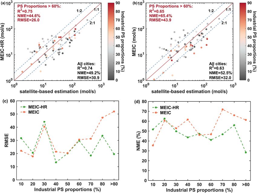
Environ. Res. Lett. 16 (2021) 084056 https://doi.org/10.1088/1748-9326/ac175f
LETTER
Improved spatial representation of a highly resolved emission
OPEN ACCESS
inventory in China: evidence from TROPOMI measurements
RECEIVED
8 June 2021 Nana Wu1, Guannan Geng2,∗, Liu Yan1, Jianzhao Bi1, Yanshun Li1, Dan Tong1, Bo Zheng3
REVISED
13 July 2021
and Qiang Zhang1
1
ACCEPTED FOR PUBLICATION Ministry of Education Key Laboratory for Earth System Modelling, Department of Earth System Science, Tsinghua University,
23 July 2021 Beijing 100084, People’s Republic of China
2
PUBLISHED
State Key Joint Laboratory of Environment Simulation and Pollution Control, School of Environment, Tsinghua University,
5 August 2021 Beijing 100084, People’s Republic of China
3
Institute of Environment and Ecology, Tsinghua Shenzhen International Graduate School, Tsinghua University, Shenzhen 518055,
People’s Republic of China
Original content from ∗
this work may be used Author to whom any correspondence should be addressed.
under the terms of the
E-mail: guannangeng@tsinghua.edu.cn
Creative Commons
Attribution 4.0 licence.
Keywords: emission inventory, high-resolution, TROPOMI
Any further distribution
of this work must Supplementary material for this article is available online
maintain attribution to
the author(s) and the title
of the work, journal
citation and DOI. Abstract
Emissions in many sources are estimated in municipal district totals and spatially disaggregated
onto grid cells using empirically selected spatial proxies such as population density, which might
introduce biases, especially in fine spatial scale. Efforts have been made to improve the spatial
representation of emission inventory, by incorporating comprehensive point source database (e.g.
power plants, industrial facilities) in emission estimates. Satellite-based observations from the
TROPOspheric Monitoring Instrument (TROPOMI) with unprecedented pixel sizes (3.5 × 7 km2 )
and signal-to-noise ratios offer the opportunity to evaluate the spatial accuracy of such highly
resolved emissions from space. Here, we compare the city-level NOx emissions from a proxy-based
emission inventory named the Multi-resolution Emission Inventory for China (MEIC) with a
highly resolved emission inventory named the Multi-resolution Emission Inventory for China -
High Resolution (MEIC-HR) that has nearly 100 000 industrial facilities, and evaluate them
through NOx emissions derived from the TROPOMI NO2 tropospheric vertical column densities
(TVCDs). We find that the discrepancies in city-level NOx emissions between MEIC and
MEIC-HR are influenced by the proportions of emissions from point sources and NOx emissions
per industrial gross domestic product (IGDP). The use of IGDP as a spatial proxy to disaggregate
industrial emissions tends to overestimate NOx emissions in cities with lower industrial emission
intensities or less industrial facilities in the MEIC. The NOx emissions of 70 cities are derived from
one year TROPOMI NO2 TVCDs using the exponentially modified Gaussian function. Compared
to the satellite-derived emissions, the cities with higher industrial point source emission
proportions in MEIC-HR agree better with space-constrained results, indicating that integrating
more point sources in the inventory would improve the spatial accuracy of emissions on city scale.
In the future, we should devote more efforts to incorporating accurate locations of emitting
facilities to reduce uncertainties in fine-scale emission estimates and guide future
policies.
1. Introduction mitigation policies and assessing their effects.
Emissions are fundamental inputs for chemical
Emission inventories have played an essential role transport models (CTMs), and their spatial pat-
in atmospheric science research and air quality terns are an important factor that determines
management, as they could support air pollution the model performance, especially at fine res-
modeling and forecasting, formulating emission olutions. Therefore, it is particularly critical to
© 2021 The Author(s). Published by IOP Publishing Ltd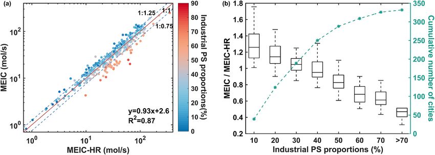
Environ. Res. Lett. 16 (2021) 084056                                                                      N Wu et al

evaluate the spatial representations of emission          the long-term (one year or more) OMI data required
inventories.                                              for NOx estimates, seasonal or subseasonal TRO-
     The traditional and widely used method to            POMI data are capable of quantifying NOx emis-
develop an emission inventory is the proxy-based          sions, and under extremely special conditions, even
method, which estimates emission totals at the muni-      data from a single day are sufficient [34]. Beirle et al
cipal level (e.g. countries or provinces) and alloc-      [33] has demonstrated that NOx emissions from large
ates them to fine grids using spatial proxies (e.g.       point sources can be mapped at high spatial resolu-
population density, nighttime light, road networks)       tion based on TROPOMI measurements and the con-
[1–6]. The proxy-based method is based on an              tinuity equation.
assumption that emissions are linearly correlated with        In this work, we first compare the city-level NOx
the selected proxies, which might introduce biases        emissions from a proxy-based emission inventory
since the energy consumption and emission level per       and a highly resolved emission inventory that con-
unit of proxies are spatially heterogeneous [7–13].       tains nearly 100 000 industrial infrastructures over
Previous studies have shown that high-resolution          China to study their differences and related impact
(
Environ. Res. Lett. 16 (2021) 084056 N Wu et al
Table 1. The emission allocation methods from provinces to cities in different sectors in MEIC-HR and MEIC. Emission magnitudes
and emission proportions by sector are also listed. The bold font represents the discrepancies between MEIC-HR and MEIC.
Province to city Emissions
Sector Subsector MEIC-HR MEIC (Tg) Proportion
Industry Boiler Point source Industrial GDP 2.66 13%
Iron Point source 2.49 12%
Cement Point source 0.92 5%
Glass Point source 0.31 2%
Other industry Industrial GDP 0.99 5%
Power — Point source 4.14 21%
Residential — Urban population/Rural population 0.85 4%
Transportation On-road Vehicle population 7.72 38%
Off-road Machine power/Total GDP/population
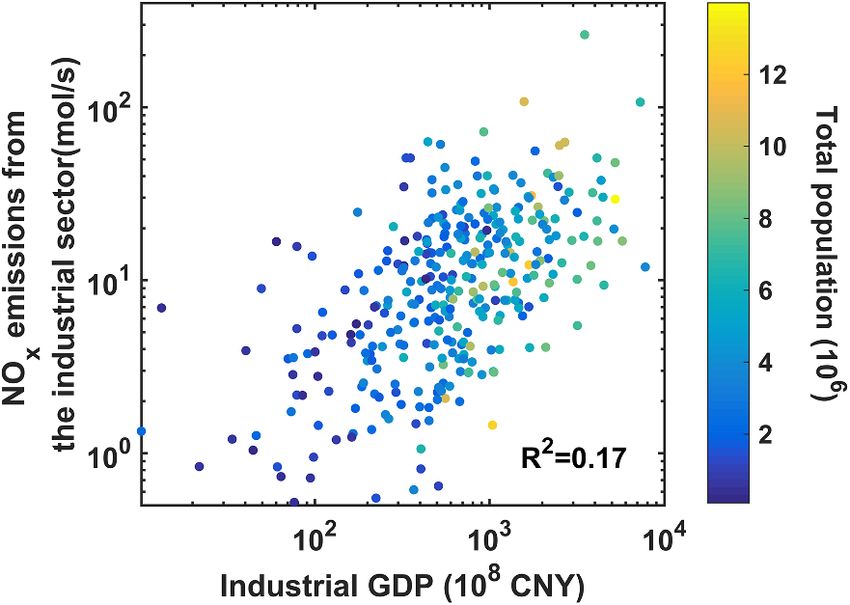
Figure 1. Comparisons between industrial NOx emissions from the point-source-based MEIC-HR and IGDP of all cities in
China. The color of symbols corresponds to the total population of each city.
(IGDP), while the MEIC-HR is mapped based on the consequence, uncertainties caused by the linear hypo-
exact locations of the industrial facilities. We define a thesis in proxy-based methods need to be evaluated.
variable as industrial point source emission propor-
tions (i.e. industrial PS proportions), which repres- 2.2. Satellite and wind data
ents the ratio of point-based emissions from boiler, TROPOMI is a payload on Sentinel-5 Precursor
iron, cement and glass in the MEIC-HR to emis- (S5P), which was launched on 13 October 2017 by
sions from all sectors. Although emissions from the the European Space Agency. The instrument achieves
power sector are also point sources, they are exactly daily global coverage with a swath width of 2600 km
the same in the two emission inventories and are not and ascends across the equator at approximately
considered in the point source proportion calcula- 13:30 local time. Compared to OMI, the significant
tion, as we mainly focus on the differences brought improvements of TROPOMI are unparalleled spa-
by the four industrial subsectors. Emission disaggreg- tial resolution of up to 3.5 × 7 km2 (upgraded to
ation for other industry, power, residential and trans- 5.5 × 3.5 km2 on 6 August 2019) and 1–5 times higher
portation in MEIC and MEIC-HR are the same. signal-to-noise ratios, which provide more details on
Although population and IGDP are widely util- a fine scale and improve the quality and reliability
ized in spatial allocations, it is worth noting that city- of the captured data. NO2 is one of the main trace
level NOx emissions from industrial sectors are not gases measured by TROPOMI, of which NO2 pro-
linearly correlated with IGDP (figure 1). IGDP data cessor realizes many retrieval improvements [38].
and population data used in this study are from China In this study, we use NO2 TVCDs over China
City Statistical Yearbook 2017 [37]. The R2 between from February 2018 to February 2019 from the
industrial NOx emissions and IGDP is 0.17, and the official TM5-MP-DOMINO version 1.0.0 L2 offline
R2 between NOx emissions from the industrial sec- product (www.temis.nl/airpollution/no2col/data/tro
tor and the total population is as low as 0.07. As a pomi/). Pixels with ‘quality assurance value’ below
3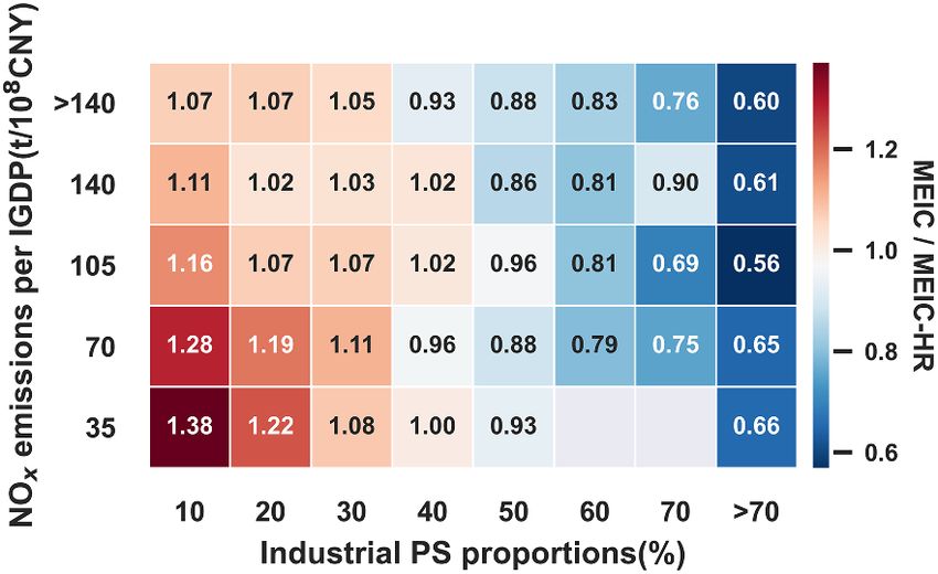
Environ. Res. Lett. 16 (2021) 084056                                                                          N Wu et al

0.75 are filtered to remove cloud radiance frac-                where N(x) represents a model function for the
tion greater than 0.5 and erroneous retrievals [38];            observed NO2 line densities (i.e. NO2 per cm), which
then, NO2 TVCDs are mapped at 0.06◦ × 0.06◦ .                   are calculated by integration of the mean NO2 TVCDs
Wind fields below 500 m with 0.36 degrees spa-                  perpendicular to the wind direction. The removal of
tial resolution and six-hour temporal resolution are            NO2 can be simply described by a first order loss and
taken from the ECMWF reanalysis (www.ecmwf.int/                 thus the truncated exponential decay function e(x)
en/research/climate-reanalysis/era-interim). Follow-            represents the chemical decay of NO2 . C(x) repres-
ing the method described in Liu et al [28], the                 ents the NO2 patterns under calm conditions, and
six hourly ECMWF wind fields are interpolated in                a, b reflect systematic deviations between windy and
time to match TROPOMI overpass time, and hori-                  calm wind, x0 is the e-folding distance downwind, w
zontal wind components are averaged in the ver-                 is the mean wind speed. A nonlinear least-squares fit
tical direction according to the weight of the layer            of N(x) is performed to derive a, b and x0 , and the
height.                                                         e-folding distance x0 is divided by the average wind
                                                                speed w to obtain the lifetime τ .
2.3. Fitting the NOx emissions and lifetimes of                      The emission rate is obtained in three steps
cities                                                          according to the mass balance (equation (4)). First,
The EMG model is used to derive the NOx emis-                   the total NO2 mass ANO2 under calm conditions
sions and atmospheric lifetimes of cities following             around the centers of emitting sources are quanti-
the method developed by Liu et al [28], which is                fied (equation (5)). We use a corrected factor f (σi )
for sources located in a heterogeneously polluted               based on the fitted width of the Gaussian plume to
background and applicable to our work. Wind fields              scale ANO2 to account for possible losses by cross-wind
are divided into calm and windy conditions with a               dilution as Liu et al [28] do (see equation (6)). Then
threshold of 2 m s−1 , as in Beirle et al [25] and Liu          NO2 is converted to NOx with a conversion coeffi-
et al [28]. The NO2 spatial distributions under calm            cient of 1.32, as suggested by Beirle et al [25] and Liu
conditions represent the spatial patterns of NOx emis-          et al [28]. Finally, the NOx mass ANOx is divided by
sions. Changes in the NO2 spatial patterns from calm            the corresponding lifetime τ to obtain NOx emission
to windy conditions indicate how long NO2 survives              rates (equation (4)). The most complicated part of
in the atmosphere. The function for the lifetime fit is         the above processes is the calculation of the total NO2
expressed as follows:                                           mass under calm conditions, and the fitting model is
                                                                as equation (5):
                N (x) = a × [e ⊗ C] (x) + b           (1)                                  ANOx
                                                                                      E=                            (4)
                                                                                            τ
                                  (    )
                                  x                                                       (            )
                    e (x) = exp −                     (2)                          1         (x − X)
                                                                                                     2
                                  x0                            gi (x) = ANO2 × √      exp −             + εi + βi x
                                                                                  2πσi          2σi2
                                  x0                                                                            (5)
                            τ=                        (3)
                                  w

                                                   (          )/
                                                       (x−X)2                   (        )
                                    ∫ 20km √ 1
                                               exp   −                            (x−X)2
                           f (σi ) = −20km 2πσi          2σ 2
                                                            i        ∫∞
                                                                      −∞ 2πσ exp − 2σ 2
                                                                        √1                                          (6)
                                                                                i           i

                                                                use 600 km as the fitting interval and 300 km as
where g(x) is a modified Gaussian function, which               the integration interval for lifetime fit, and we set a
is for NO2 line densities (i.e. NO2 per cm) under               fitting interval of 200 km (300 km for Pearl River
calm wind, i represents the wind directions of rota-            Delta) and an integration interval of 40 km (60 km
tion, ANOx and ANO2 are the NOx amount and NO2                  for Pearl River Delta) for total NO2 mass fit. Strict
amount, respectively, X is the location of inversion            constraints are set on fit performance, as shown in
sites, εi and βi indicate the hypothesis of a linear dis-       Liu et al [28]: R ⩾ 0.9, confidence intervals of life-
tribution of background concentrations, and σi rep-             time 0. The fitting model shows robust ability to
ods to calculate the lifetimes and emissions of cit-            derive the lifetimes and emissions of cities. Uncertain-
ies. In accordance with the set in Liu et al [28], we           ties resulting from the parameters used in the model

                                                  4
Environ. Res. Lett. 16 (2021) 084056 N Wu et al
Figure 2. Comparisons of the city-level NOx emissions between MEIC and MEIC-HR. (a) Correlations between city-level NOx
emissions in MEIC and those in MEIC-HR. The colors of the symbols correspond to the industrial PS proportions. The dotted
line and two dashed lines represent slopes of 1.0, 0.75 and 1.25, respectively. (b) Changes of MEIC/MEIC-HR ratio as a function
of industrial PS proportions. The boxplot represents the median, upper quartile, and lower quartile of MEIC/MEIC-HR ratio.
The green line shows the cumulative number of cities.
and other factors for the lifetime and emission fit are regions. Figure 3 presents the discrepancies of city-
presented in section 4.1. In addition, sites with an level NOx emissions between MEIC and MEIC-HR
elevation difference of more than 250 m in ECMWF and their relationships with IGDP and industrial PS
and GTOPO30 (https://earthexplorer.usgs.gov/) are proportions in each city. In a certain industrial PS
defined as mountainous cities and eliminated in our proportion range, the average MEIC/MEIC-HR ratio
analysis, as in Liu et al [28]. decreases along with the increase in NOx emissions
per IGDP. For example, when industrial PS propor-
tions are less than 10%, the average MEIC/MEIC-HR
3. Results ratio declines from 1.38 to 1.07 as the NOx emis-
sions per IGDP increase from 35 to over 140 t/108
3.1. City-level NOx emissions in the two emission
CNY. Compared to the real-world emissions, the
inventories
assumption that NOx emissions are linearly associ-
Figure 2(a) compares the city-level NOx emissions
ated with IGDP tends to allocate more/less emis-
from MEIC and MEIC-HR. Although the R2 value
sions to cities with low/high emission intensities,
reaches 0.87, most cities deviate from the 1:1 line,
which results in overestimation/underestimation of
among which 96 cities deviate by more than 25%,
NOx emissions in the MEIC. Similarly, in a cer-
accounting for approximately 39% of the total cities.
tain range of NOx emissions per IGDP, the average
This result indicates that different spatial disaggrega-
MEIC/MEIC-HR ratio decreases as industrial PS pro-
tion methods lead to city-level emission discrepancies
portions increase. For example, when the NOx emis-
considering that provincial NOx emissions in MEIC
sions per IGDP are between 35 and 70 t/108 CNY,
and MEIC-HR are the same. The differences between
the average MEIC/MEIC-HR decreases from 1.28 to
city-level NOx emissions in MEIC and MEIC-HR are
0.65 as industrial PS proportions increase from 10%
related to the industrial PS proportions in each city,
to over 70%. As the industrial PS proportions defined
with cities of high industrial PS proportions below
in our study are from highly polluting industries such
the 1:1 line and vice versa. Figure 2(b) further ana-
as iron and cement, lower industrial PS proportions
lyzes the ratio of NOx emissions in the MEIC to those
under a certain range of emission intensity reflect
in the MEIC-HR (MEIC/MEIC-HR) as a function
that the IGDP in those cities are contributed more by
of industrial PS proportions. The MEIC/MEIC-HR
other cleaning industries. Therefore, using IGDP to
ratio decreases with the median value from 1.26 to
allocate emissions from province level to cities tend to
0.47 as the industrial PS proportions increase from
overestimate the industrial emissions of such cities.
10% to more than 70%, indicating that the proxy-
based inventory (MEIC) tends to overestimate the
NOx emissions for cities with lower industrial PS pro- 3.2. City-level NOx emissions derived from satellite
portions and underestimate the NOx emissions for observations
cities occupied by a large amount of industrial factor- We apply the EMG model described in section 2.3
ies (i.e. higher industrial PS proportions). and finally derive the NOx lifetimes and emissions
In the MEIC, IGDP is used as the spatial proxy of 70 cities in China from TROPOMI measurements
to allocate industrial NOx emissions from province (table S1 (available online at stacks.iop.org/ERL/16/
level to cities/counties, which may induce biases since 084056/mmedia)). High spatial resolution and low
NOx emissions per IGDP are heterogeneous among noise enable TROPOMI to have more effective pixels
5Environ. Res. Lett. 16 (2021) 084056 N Wu et al
Figure 3. The relationships of MEIC/MEIC-HR ratio with NOx emissions per IGDP and industrial PS proportions in each city.
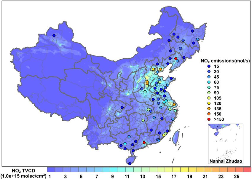
Figure 4. Average TROPOMI NO2 TVCDs over China from February 2018 to February 2019 overlaid with the locations of cities
with successfully derived emissions in this work, and their colors indicate the derived NOx emissions.
and exhibits a significantly better performance of The fitted NOx lifetimes range from 1.0 h to 9.3 h
representing spatial variability than any instrument in this work, which correspond to the results repor-
before it [39, 40], which increases the possibility of ted in the literature [24–26, 28]. The city with the
meeting the constraints on model performance (see highest NOx emissions rate is Pearl River Delta (up
the last paragraph of section 2.3 for details). As the key to 331 mol s−1 ), while the lowest is Wuzhou (only
for deriving NOx lifetimes and emissions is to ensure 2 mol s−1 ). Figure 4 presents the spatial distributions
strong gradients of the NO2 signal around the source, of the average NO2 TVCDs over China from Febru-
the improved estimation of NOx lifetimes and emis- ary 2018 to February 2019 overlaid with the derived
sions by high-quality satellite measurements is dir- NOx emissions of 70 cities. Hotspots of average NO2
ectly reflected in the greater number of derived cities TVCDs are mainly located in the North China Plain,
compared to previous works [28]. Yangtze River Delta, Pearl River Delta, Fenwei Plain
6Environ. Res. Lett. 16 (2021) 084056 N Wu et al
Figure 5. Comparisons of city-level NOx emissions between satellite-based estimates and the two emission inventories.
(a) Correlations between city-level NOx emissions in MEIC-HR and satellite-based estimates. The color of each symbol
corresponds to the industrial PS proportions. We calculated the statistical indicators for all cities and the cities with industrial PS
proportions more than 60%: R is the correlation coefficient, RMSE is the root mean square error, and NME is the normalized
mean error. The dotted line and two dashed lines represent slopes of 1.0, 0.5 and 2.0, respectively. (b) The same as (a), but for
MEIC. (c) The RMSE under different segments of industrial PS proportions. (d) The NME under different segments of industrial
PS proportions.
and Sichuan-Chongqing region, which are consist- Figures 5(c) and (d) further show a comparison
ent with the spatial patterns of NOx emissions of the between NOx emissions in emission inventories and
investigated cities in this study. satellite-based estimates as a function of industrial PS
proportions. When industrial PS proportions are rel-
atively low (60%), the root mean square the highly resolved emission inventories have better
error (RMSE) is 26.0 and 43.9 mol s−1 for MEIC- spatial representations of real-world emission distri-
HR and MEIC, respectively, and the normalized mean butions than proxy-based inventories, especially in
error (NME) is 44.6% and 65.4%, respectively. regions with a large amount of emitting facilities. It
7Environ. Res. Lett. 16 (2021) 084056 N Wu et al
is crucial to raise point source emission proportions consideration and conclude that the total uncertain-
in emission inventories to reduce spatial biases caused ties of lifetimes and emissions are within 42%–91%
by spatial proxies. and 57%–99%, respectively. This uncertainty range is
comparable to Liu et al [28] and Liu et al [31]. As illus-
4. Discussion trated in Liu et al [28] and Liu et al [31], under the
assumption that all uncertain factors are independ-
4.1. Uncertainties ent, the total uncertainty calculated here is rather con-
There are several uncertainties in this work. Liu servative.
et al [28] systematically evaluated the uncertainties
in the EMG model. Here, following Liu et al [28], 4.2. Implications
we estimate the uncertainties of the NOx lifetimes In this study, we use NOx emissions derived from
and emissions from six aspects: (a) sensitivity tests TROPOMI NO2 TVCDs to evaluate the NOx emis-
are conducted to quantify the uncertainties from sions on city scale estimated from two bottom-up
the choice of fit and integration intervals. The fit- emission inventories. NOx is selected as an example
ted lifetimes and emissions are found to be insens- here because the errors in NO2 satellite retrievals
itive to the choice of the fit and integration inter- are relatively small [41, 45, 46] and the method to
vals. Table S2 shows that for the lifetime fit, every derive NOx emissions in cities from satellite data is
100 km changes of the fit interval f or integration solid [25, 28, 31, 34, 47]. The findings obtained in
interval i cause lifetimes to vary by about 10%. For this work that raising point emission proportions in
the total NO2 mass fit, 10% or 20% changes of the emission inventory could improve its spatial repres-
fit interval h or integration interval v lead to less entation on city scale are also applicable to other air
than 20% changes of NOx emission rates. (b) The pollutant species (e.g. CO2 and SO2 ) from fossil fuel
95% confidence interval and the standard mean error combustion, as they come from the same emission
of the lifetimes under different wind directions are sources.
used to quantify the fit errors for each investigated Recently, some studies have emphasized the
site. (c) With the consideration of the height of wind importance of spatial allocation method in the devel-
fields and threshold for calm winds, the wind fields opment of gridded emissions [7, 14–16, 18, 19].
from ECMWF lead to an uncertainty of ∼30% for For example, Zheng et al [18] compile the MEIC-
non-mountainous cities. (d) In this study, we use HR inventory with comprehensive industrial-facility-
a constant scaling factor of 1.32 to convert NO2 to level information and find that the point-source-
NOx , which is a typical value under cloud-free con- based emission inventory substantially improves the
ditions around noon when polluted air masses sup- WRF/CMAQ model simulations at high spatial res-
port the formation of O3 (i.e. TROPOMI overpass olution of 4 km compared to the proxy-based emis-
time). Although the difference in O3 concentrations sions. Our study adds new evidence from space to
between upwind and downwind plumes might influ- prove the accuracy of the spatial patterns represented
ence NOx /NO2 , the effect has been included in the by such highly resolved emission inventory. However,
overall uncertainty estimates as we average the fit res- due to the limitation of the emission retrieval method,
ults for different wind direction sectors, which usually only 70 cities are covered in our evaluation analysis. A
represent different incoming O3 concentrations. The more comprehensive evaluation in the future might
constant NOx /NO2 scaling factor brings an uncer- be comparing modeled tropospheric vertical columns
tainty of ∼10% to the derived emissions (but not life- from CTMs at fine spatial resolution with TVCDs
times) based on previous studies [25, 28, 31, 33]. (e) with unprecedented resolution from TROPOMI, fol-
The uncertainty of TVCDs is ∼30% according to pre- lowing the method in Geng et al [15].
vious studies [39, 41–43], which directly propagates As reported in previous studies [11, 14, 16–18],
to NO2 amount and thus the estimated emissions (but emissions from point sources exhibit inconsistent
not lifetimes). The uncertainty of TVCDs consists of spatial patterns with those from spatial proxies (e.g.
additive and multiplicative terms. The uncertainty population density) at fine spatial scale, which means
of multiplicative terms comes from tropospheric air- the decoupling effect between emission inventory
mass factor, which depends on profile shape, cloud constructed from large point database and spatial
parameters, albedo and surface pressure [44]. And proxies. More importantly, the spatial patterns of
the uncertainty of TVCDs from additive components such highly resolved inventory cannot be repro-
owing to the spectral retrieval and stratospheric cor- duced by any spatial proxies that have been fre-
rection is eliminated by the fitted background in our quently used before. Therefore, it is crucial to
study. (f) The wind speed is an important impact increase the share of point source emissions by
factor for the fitted lifetime [26], which is assumed including more detailed point source statistical data
to be the same under calm and windy conditions in [11, 14, 16–18], conducting field surveys [17, 24, 48]
this work. The systematic difference of NO2 TVCDs or identifying missing point sources by means of
between calm and windy conditions is about 20% satellite observations [29, 49, 50]. For example, three
(figure S1). We take the factors mentioned above into industrial datasets are combined in MEIC-HR to
8Environ. Res. Lett. 16 (2021) 084056 N Wu et al
provide a synthesized facility-level database [18]. better agreement with satellite-based estimates than
To develop high-resolution emission inventory, on- those in MEIC (r 2 = 0.63). And the improvement is
site surveys for industrial sources are conducted to more obvious for cities with high industrial PS pro-
obtain key parameters relevant to emission estima- portions (>60%), which is manifested as the RMSE
tion [17, 24, 48]. Owing to the wide spatial cover- is 26.0 and 43.9 mol s−1 for MEIC-HR and MEIC,
age, high temporal and spatial resolution, and timely respectively, and the NME is 44.6% and 65.4% for
updates, satellite data can be used to detect emis- MEIC-HR and MEIC, respectively, indicating that
sion sources including those that are not captured in incorporating comprehensive point source database
bottom-up emission inventories due to lack of avail- will improve the spatial representation of emission
able data, especially in developing nations. Mclinden inventories.
et al [29] use the measurement of SO2 from OMI and This work emphasizes the importance of integ-
find nearly 40 emission sources missing from conven- rating more point sources in emission inventories
tional inventories, accounting for roughly 6%–12% to improve the spatial accuracy. Our study provides
of the global anthropogenic source. The combination a framework to propagate top-down information
of bottom-up and top-down information might lead from satellite to the evaluations of bottom-up invent-
to greater accuracy of fine scale emission inventory in ories, which could support the development and
the future. refinement of highly resolved emission inventor-
ies in the future. More efforts should be made
5. Conclusion to develop highly resolved emission inventories
to facilitate atmospheric research and air quality
The proxy-based method to allocate emission totals management.
to smaller administrative districts or grids might
introduce biases, especially at fine scales. Develop- Data availability statement
ing highly resolved emission inventories is an effective
way to support fine-scale emission characterization, The data that support the findings of this study are
whose improvement to the spatial representations available upon reasonable request from the authors.
of emissions needs to be studied. In this work, we
evaluate the effect of integrating a large amount of Acknowledgments
point sources on emission allocations from province
level to cities using a proxy-based emission invent- This work was supported by the National Natural Sci-
ory (MEIC), a highly resolved emission invent- ence Foundation of China (91744310 and 42005135).
ory (MEIC-HR), and satellite observations. We first
investigate the discrepancies in city-level NOx emis- ORCID iDs
sions between the two emission inventories and dia-
gnose the related impact factors. City-level NOx emis- Guannan Geng https://orcid.org/0000-0002-
sions derived from TROPOMI NO2 TVCDs are then 1605-8448
applied to evaluate the spatial representations of city- Bo Zheng https://orcid.org/0000-0001-8344-3445
level emissions by MEIC and MEIC-HR.
We find that the discrepancies in city-level NOx References
emissions between MEIC and MEIC-HR are affected
[1] Streets D G et al 2003 An inventory of gaseous and primary
by the industrial PS proportions and NOx emis-
aerosol emissions in Asia in the year 2000 J. Geophys. Res.
sions per IGDP. As the industrial PS proportions Atmos. 108 8809
increase from 10% to over 70%, the median value of [2] Shi K, Chen Y, Yu B, Xu T, Chen Z, Liu R, Li L and Wu J 2016
MEIC/MEIC-HR ratio decreases from 1.26 to 0.47. Modeling spatiotemporal CO2 (carbon dioxide) emission
dynamics in China from DMSP-OLS nighttime stable light
When NOx emissions per IGDP are in a certain range,
data using panel data analysis Appl. Energy 168 523–33
the mean MEIC/MEIC-HR ratio decreases along with [3] Li M et al 2017 MIX: a mosaic Asian anthropogenic emission
the increase of industrial PS proportions. Similarly, inventory under the international collaboration framework
in a certain range of industrial PS proportions, the of the MICS-Asia and HTAP Atmos. Chem. Phys. 17 935–63
[4] Zheng B, Huo H, Zhang Q, Yao Z L, Wang X T, Yang X F,
mean MEIC/MEIC-HR ratio declines as NOx emis-
Liu H and He K B 2014 High-resolution mapping of vehicle
sions per IGDP increase. Therefore, Using IGDP as emissions in China in 2008 Atmos. Chem. Phys. 14 9787–805
a spatial proxy to allocate provincial industrial NOx [5] Zhang Q et al 2009 Asian emissions in 2006 for the NASA
emissions to cities tends to overestimate emissions INTEX-B mission Atmos. Chem. Phys. 9 5131–53
[6] Lu Z, Zhang Q and Streets D G 2011 Sulfur dioxide and
in cities with lower industrial PS proportions (a
primary carbonaceous aerosol emissions in China and India,
less amount of industrial facilities or lower indus- 1996–2010 Atmos. Chem. Phys. 11 9839–64
trial emission intensities). NOx emissions of 70 cit- [7] Gurney K R, Mendoza D L, Zhou Y, Fischer M L, Miller C C,
ies are derived based on TROPOMI NO2 TVCDs and Geethakumar S and de la Rue du Can S 2009 High resolution
fossil fuel combustion CO2 emission fluxes for the United
the EMG model and applied to evaluate the spa-
States Environ. Sci. Technol. 43 5535–41
tial accuracy of the two emission inventories. City- [8] Rayner P J, Raupach M R, Paget M, Peylin P and Koffi E 2010
level NOx emissions in MEIC-HR (r 2 = 0.74) show A new global gridded data set of CO2 emissions from fossil
9Environ. Res. Lett. 16 (2021) 084056 N Wu et al
fuel combustion: methodology and evaluation J. Geophys. [26] Valin L C, Russell A R and Cohen R C 2013 Variations of OH
Res. Atmos. 115 D19306 radical in an urban plume inferred from NO2 column
[9] Zhou Y and Gurney K R 2011 Spatial relationships of measurements Geophys. Res. Lett. 40 1856–60
sector-specific fossil fuel CO2 emissions in the United States [27] Fioletov V E, McLinden C A, Krotkov N and Li C 2015
Glob. Biogeochem. Cycles 25 GB3002 Lifetimes and emissions of SO2 from point sources estimated
[10] Nassar R, Napier-Linton L, Gurney K R, Andres R J, Oda T, from OMI Geophys. Res. Lett. 42 1969–76
Vogel F R and Deng F 2013 Improving the temporal and [28] Liu F, Beirle S, Zhang Q, Dörner S, He K and Wagner T 2016
spatial distribution of CO2 emissions from global NOx lifetimes and emissions of cities and power plants in
fossil fuel emission data sets J. Geophys. Res. Atmos. polluted background estimated by satellite observations
118 917–33 Atmos. Chem. Phys. 16 5283–98
[11] Oda T and Maksyutov S 2011 A very high-resolution [29] McLinden C A, Fioletov V, Shephard M W, Krotkov N, Li C,
(1 km × 1 km) global fossil fuel CO2 emission inventory Martin R V, Moran M D and Joiner J 2016 Space-based
derived using a point source database and satellite detection of missing sulfur dioxide sources of global air
observations of nighttime lights Atmos. Chem. Phys. pollution Nat. Geosci. 9 496–500
11 543–56 [30] Liu F, Duncan B N, Krotkov N A, Lamsal L N, Beirle S,
[12] Gately C K, Hutyra L R, Wing I S and Brondfield M N 2013 Griffin D, McLinden C A, Goldberg D L and Lu Z 2020 A
A bottom up approach to on-road CO2 emissions estimates: methodology to constrain carbon dioxide emissions from
improved spatial accuracy and applications for regional coal-fired power plants using satellite observations of
planning Environ. Sci. Technol. 47 2423–30 co-emitted nitrogen dioxide Atmos. Chem. Phys.
[13] Gately C K, Hutyra L R and Sue Wing I 2015 Cities, traffic, 20 99–116
and CO2 : a multidecadal assessment of trends, drivers, and [31] Liu F, Beirle S, Zhang Q, van der A R J, Zheng B, Tong D and
scaling relationships Proc. Natl Acad. Sci. 112 4999–5004 He K 2017 NOx emission trends over Chinese cities
[14] Zheng B, Zhang Q, Tong D, Chen C, Hong C, Li M, Geng G, estimated from OMI observations during 2005–2015 Atmos.
Lei Y, Huo H and He K 2017 Resolution dependence of Chem. Phys. 17 9261–75
uncertainties in gridded emission inventories: a case study in [32] Veefkind J P et al 2012 TROPOMI on the ESA sentinel-5
Hebei, China Atmos. Chem. Phys. 17 921–33 precursor: a GMES mission for global observations of the
[15] Geng G, Zhang Q, Martin R V, Lin J, Huo H, Zheng B, atmospheric composition for climate, air quality and ozone
Wang S and He K 2017 Impact of spatial proxies on the layer applications Remote Sens. Environ. 120 70–83
representation of bottom-up emission inventories: a [33] Beirle S, Borger C, Dörner S, Li A, Hu Z, Liu F, Wang Y and
satellite-based analysis Atmos. Chem. Phys. 17 4131–45 Wagner T 2019 Pinpointing nitrogen oxide emissions from
[16] Zheng H, Cai S, Wang S, Zhao B, Chang X and Hao J 2019 space Sci. Adv. 5 eaax9800
Development of a unit-based industrial emission inventory [34] Goldberg D L, Lu Z, Streets D G, de Foy B, Griffin D,
in the Beijing–Tianjin–Hebei region and resulting McLinden C A, Lamsal L N, Krotkov N A and Eskes H 2019
improvement in air quality modeling Atmos. Chem. Phys. Enhanced capabilities of TROPOMI NO2 : estimating NOX
19 3447–62 from North American Cities and power plants Environ. Sci.
[17] Zhou Y, Zhao Y, Mao P, Zhang Q, Zhang J, Qiu L and Yang Y Technol. 53 12594–601
2017 Development of a high-resolution emission inventory [35] Li M et al 2017 Anthropogenic emission inventories in
and its evaluation and application through air quality China: a review Nat. Sci. Rev. 4 834–66
modeling for Jiangsu Province, China Atmos. Chem. Phys. [36] Zheng B et al 2018 Trends in China’s anthropogenic
17 211–33 emissions since 2010 as the consequence of clean air actions
[18] Zheng B, Cheng J, Geng G, Wang X, Li M, Shi Q, Qi J, Lei Y, Atmos. Chem. Phys. 18 14095–111
Zhang Q and He K 2021 Mapping anthropogenic emissions [37] National Bureau of Statistics of People’s Republic of China
in China at 1 km spatial resolution and its application in air 2017 China City Statistical Yearbook 2017 (Beijing: China
quality modeling Sci. Bull. 66 612–20 Statistics Press)
[19] Wang Y, Wang J, Zhou M, Henze D K, Ge C and Wang W [38] van Geffen J H G M, Eskes H J, Boersma K F, Maasakkers J D
2020 Inverse modeling of SO2 and NOx emissions over and Veefkind J P 2019 TROPOMI ATBD of the total and
China using multisensor satellite data—part 2: downscaling tropospheric NO2 data products (S5P-KNMI-L2-0005-RP,
techniques for air quality analysis and forecasts Atmos. Royal Netherlands Meteorological Institute) (available at:
Chem. Phys. 20 6651–70 https://sentinel.esa.int/documents/247904/2476257/
[20] Xiong T, Jiang W and Gao W 2016 Current status and Sentinel-5P-TROPOMI-ATBD-NO2-data-products)
prediction of major atmospheric emissions from coal-fired (accessed 23 April 2020)
power plants in Shandong Province, China Atmos. Environ. [39] Griffin D et al 2019 High-resolution mapping of nitrogen
124 46–52 dioxide with TROPOMI: first results and validation over the
[21] Liu F, Zhang Q, Tong D, Zheng B, Li M, Huo H and He K B Canadian oil sands Geophys. Res. Lett. 46 1049–60
2015 High-resolution inventory of technologies, activities, [40] Wang C, Wang T, Wang P and Rakitin V 2020 Comparison
and emissions of coal-fired power plants in China from 1990 and validation of TROPOMI and OMI NO2 observations
to 2010 Atmos. Chem. Phys. 15 13299–317 over China Atmosphere 11 636
[22] Wang K, Tian H, Hua S, Zhu C, Gao J, Xue Y, Hao J, Wang Y [41] Boersma K, Eskes H and Brinksma E 2004 Error analysis for
and Zhou J 2016 A comprehensive emission inventory of tropospheric NO2 retrieval from space J. Geophys. Res.
multiple air pollutants from iron and steel industry in China: 109 D04311
temporal trends and spatial variation characteristics Sci. [42] Lorente A et al 2017 Structural uncertainty in air mass factor
Total Environ. 559 7–14 calculation for NO2 and HCHO satellite retrievals Atmos.
[23] Qi J, Zheng B, Li M, Yu F, Chen C, Liu F, Zhou X, Yuan J, Meas. Tech. 10 759–82
Zhang Q and He K 2017 A high-resolution air pollutants [43] Lorente A, Boersma K F, Eskes H J, Veefkind J P, Van Geffen J
emission inventory in 2013 for the Beijing-Tianjin-Hebei H G M, De Zeeuw M B, Denier van der Gon H A C, Beirle S
region, China Atmos. Environ. 170 156–68 and Krol M C 2019 Quantification of nitrogen oxides
[24] Zhao Y, Xia Y and Zhou Y 2018 Assessment of a emissions from build-up of pollution over Paris with
high-resolution NOx emission inventory using satellite TROPOMI Sci. Rep. 9 20033
observations: a case study of southern Jiangsu, China Atmos. [44] McLinden C A, Fioletov V, Boersma K F, Kharol S K,
Environ. 190 135–45 Krotkov N, Lamsal L, Makar P A, Martin R V, Veefkind J P
[25] Beirle S, Boersma K F, Platt U, Lawrence M G and Wagner T and Yang K 2014 Improved satellite retrievals of NO2 and
2011 Megacity emissions and lifetimes of nitrogen oxides SO2 over the Canadian oil sands and comparisons with
probed from space Science 333 1737–9 surface measurements Atmos. Chem. Phys. 14 3637–56
10Environ. Res. Lett. 16 (2021) 084056 N Wu et al
[45] Van Geffen J, Boersma K F, Eskes H, Sneep M, Ter Linden M, [48] Zhao Y et al 2015 Advantages of a city-scale emission
Zara M and Veefkind J P 2020 S5P TROPOMI NO2 slant inventory for urban air quality research and policy: the case
column retrieval: method, stability, uncertainties and of Nanjing, a typical industrial city in the Yangtze River
comparisons with OMI Atmos. Meas. Tech. 13 1315–35 Delta, China Atmos. Chem. Phys. 15 12623–44
[46] Boersma K F et al 2011 An improved tropospheric NO2 [49] Liu F et al 2018 A new global anthropogenic SO2 emission
column retrieval algorithm for the Ozone monitoring inventory for the last decade: a mosaic of satellite-derived
instrument Atmos. Meas. Tech. 4 1905–28 and bottom-up emissions Atmos. Chem. Phys. 18 16571–86
[47] Lu Z, Streets D G, De Foy B, Lamsal L N, Duncan B N and [50] Luo J, Han Y, Zhao Y, Liu X, Huang Y, Wang L, Chen K,
Xing J 2015 Emissions of nitrogen oxides from US urban Tao S, Liu J and Ma J 2020 An inter-comparative evaluation
areas: estimation from Ozone monitoring instrument of PKU-FUEL global SO2 emission inventory Sci. Total
retrievals for 2005–2014 Atmos. Chem. Phys. 15 10367–83 Environ. 722 137755
11You can also read