GTPack: A Mathematica group theory package for application in solid-state physics and photonics
←
→
Page content transcription
If your browser does not render page correctly, please read the page content below
GTPack: A Mathematica group theory
                                                    package for application in solid-state physics
                                                    and photonics
                                                    R. Matthias Geilhufe 1,∗ and Wolfram Hergert 2
                                                    1 Nordita,  KTH Royal Institute of Technology and Stockholm University,
                                                    Roslagstullsbacken 23, SE-106 91 Stockholm, Sweden
                                                    2 Institute of Physics, Martin Luther University Halle-Wittenberg,
arXiv:1807.01245v1 [cond-mat.mtrl-sci] 3 Jul 2018

                                                    Von-Seckendorff-Platz 1, 06120 Halle, Germany
                                                    Correspondence*:
                                                    R. M. Geilhufe, W. Hergert
                                                    geilhufe@kth.se, wolfram.hergert@physik.uni-halle.de

                                                    ABSTRACT
                                                      We present the Mathematica group theory package GTPack providing about 200 additional
                                                    modules to the standard Mathematica language. The content ranges from basic group theory
                                                    and representation theory to more applied methods like crystal field theory, tight-binding and
                                                    plane-wave approaches capable for symmetry based studies in the fields of solid-state physics
                                                    and photonics. GTPack is freely available via http://GTPack.org. The package is designed
                                                    to be easily accessible by providing a complete Mathematica-style documentation, an optional
                                                    input validation and an error strategy. We illustrate the basic framework of the package and
                                                    show basic examples to present the functionality. Furthermore, we give a complete list of the
                                                    implemented commands including references for algorithms within the supplementary material.

                                                    INTRODUCTION
                                                    Symmetry and symmetry breaking are basic concepts of nature. Thus, arguments based on the symmetry
                                                    of the considered system play a significant role within almost all branches of physics. Group theory
                                                    represents the mathematical language to deal with symmetry, since all transformations that leave a
                                                    physical system invariant (usually described in terms of transformations of algebraic or differential
                                                    equations) naturally form a group. The application of group theory in physics has a long tradition ranging
                                                    back to the beginning of the 20th century [1, 2]. Concentrating on solid-state and condensed matter
                                                    physics, examples for the application of group theory can be found in the theory of the degeneracy
                                                    of energy bands [3], color centers, d0 magnetism and impurity states [4, 5, 6], optical transitions [7],
                                                    phase transitions, atoms and molecules on surfaces [8], x-ray diffraction and crystallography in Fourier
                                                    space [9], construction of effective low-energy excitation Hamiltonians [10], the classification of the
                                                    superconducting states of matter [11, 12, 13, 14, 15], and, more recently, topological band theory
                                                    [16, 17, 18, 19, 20] and topological quantum computation [21]. Due to the similarity of the underlying
                                                    formalism, several concepts can be transferred to the field of photonics, for example, the band theory of
                                                    photonic crystals [22, 23, 24], impurities and defect modes [25], and selection rules and uncoupled modes
                                                    [26, 27].

                                                                                                                                                            1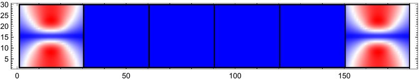
R. M. Geilhufe & W. Hergert                                       GTPack: A Mathematica group theory package

  In many cases, non-trivial results can be obtained from basic group theoretical information like the
characters of the irreducible representations or the Clebsch-Gordan coefficients. In the past decades these
information were tabulated in various books (e.g., [28, 29]). A comprehensive and widely used online
group theory tool is provided by the Bilbao crystallographic server [30]. The work with printed group
theory tables is not suitable for automation and the probability of copying and pasting misprints is high.
However, modern computer algebra systems are capable to provide the same information, assumed that the
necessary algorithms are implemented. Especially, the computer algebra system GAP (groups, algorithms
and programming) [31] represents a powerful program to deal with computationally demanding questions
in abstract algebra. Similarly, the computer algebra system Mathematica is well established within the
research community. However, a stable group theory package designed for applications in solid-state
physics and photonics is not included in the standard version.
  The development of the Mathematica group theory package GTPack was designed to fill this gap. The
functionality was planned to cover both, an application in active research and an application in university
teaching. Therefore a main focus is the development of a user-friendly application, via self-explanatory
names for new commands, a comprehensive documentation system and an optional input validation.
  The aim of the paper is to report on the initial version of the Mathematica group theory package GTPack
which is freely available for academic usage via http://GTPack.org. In the first part of the paper
we introduce the main functionality and structure of the package. Afterwards we give general information
about the implementation of the commands. In the last part we provide simple examples to illustrate
the package. The supplementary material contains a full reference of all implemented modules. A more
comprehensive guide about applied group theory in connection to GTPack can be found in Ref. [32].

FUNCTIONALITY AND STRUCTURE
According to the functionality of the modules, GTPack is divided into various subpackages as illustrated
in Fig. 1. In general, the subpackages can be assembled in three groups, “basic functionality”, “structure”
and “applications”. Subpackages belonging to the class of “basic functionality” are Auxiliary.m, Basic.m,
Install.m and RepresentationTheory.m. The package Auxiliary.m contains modules which are needed by
GTPack or extend the general Mathematica language. Among others tesseral harmonics (real spherical
harmonics) were added and also the Cartesian form of tesseral and spherical harmonics was implemented.
Furthermore, the package contains modules for the handling with quaternions, the calculation of Gaunt
coefficients, Dirac matrices or SU(2)-rotation matrices, to name but a few. The package Basic.m
concentrates on general abstract group theory and, for example, provides modules for the calculation
of classes, multiplication tables, left and right cosets and several logical commands to check for groups,
Abelian groups, subgroups or invariant subgroups. Modules needed for basic representation theory are

GTPack databases                                                                                  External data
Crystal field rl                                      GTPack                                      CIF files
                                                                                                  POSCAR files
Crystal structures                                                                                XSF files
Molecular structure          Basic functionality      Structure            Application
Tight-binding parameters                                                                          MPB calculations
Pseudopotential parameters   Auxiliary.m              CrystalStructure.m   CrystalField.m         Abinit calculations
                             Basic.m                  Lattice.m            ElectroniStructure.m
                             Install.m                Molecules.m          Photonics.m
                             RepresentationTheory.m                        PseudoPotential.m
                                                                           TightBinding.m
                                                                           Vibrations.m

Figure 1. Subpackage structure of GTPack and interaction with external data.

                                                                                                                        2
R. M. Geilhufe & W. Hergert GTPack: A Mathematica group theory package contained in the package RepresentationTheory.m. This package comprises the calculation of character tables, handling of irreducible representations, the calculation of Clebsch-Gordan coefficients, etc.. Modules for the installation of point and space groups or symmetry elements can be found in Install.m. The second class “structure” comprises of the packages CrystalStructure.m, Lattice.m and Molecules.m. Within CrystalStructure.m, modules for loading, saving and handling of crystal structures can be found. Modules with similar functionality but specialized on molecules are contained within Molecules.m. The construction and manipulation of atomic clusters as well as several commands for dealing with the reciprocal space are summarized in the package Lattice.m. Next to basic group theory GTPack also contains subpackages for particular applications in solid state physics and photonics. The third class “Applications” contains the subpackages CrystalField.m, ElectronicStructure.m, Photonics.m, PseudoPotential.m, TightBinding.m and Vibrations.m. The crystal field package CrystalField.m is capable of automatically generating crystal field Hamiltonians. Furthermore, it contains the generation of standard operator equivalents like Stevens [? ] and Buckmaster- Smith-Thornley [33] operators. GTPack also allows for electronic structure calculations for periodic systems, i.e. crystals, in the framework of the tight-binding and the pseudopotential approximation. Modules to construct tight-binding Hamiltonians are summarized in TightBinding.m and modules for the pseudopotential approximation in PseudoPotential.m. The calculation of band structures, density of states as well as the calculation of a Fermi surface is practically independent of the underlying model Hamiltonian. Therefore such commands are contained within the package ElectronicStructure.m. In the framework of plane-waves it is also possible to calculate the band structure of photonic crystals. The necessary modules for the construction of the master equation for various geometrical objects can be found in the package Photonics.m. Commands for the investigation of phonons or molecular vibrational modes are contained in Vibrations.m. For various applications it is necessary to incorporate data, for example, tight-binding parameters, crystal field parameters and crystal structures. Therefore, GTPack contains several modules for the creation and handling of databases (cf. Fig. 1). Here, special file endings are used, such as *.parm and *.struc. Databases can be easily created, extended and modified by the user. Furthermore, GTPack includes commands for the interaction with external data formats and ab initio software. This concerns the import and export of structural data files *.cif [34] and *.xsf [35] and the output of the programs MIT Photonic Bands - MPB [36, 37]. For the future it is intended to implement similar modules for VASP [38] and abinit [39]. IMPLEMENTATION To distinguish new commands provided by GTPack from the standard Mathematica language and to prevent conflicts with new versions of Mathematica, all GTPack commands are starting with the characters GT (e.g. GTInstallGroup, GTCharacterTable, ...). Options are denoted with a suffix GO (e.g. GOVerbose, GOIrepNotation, ...). One of the main features of GTPack is the symbolic representation of symmetry elements. Symmetry elements for various standard axes (see Figure 2)) are predefined and the respective symbols, such as C3z for a 3-fold rotation about the z-axis are protected. As a standard form they are displayed with subscripts, i.e., C3z . Internally all symmetry elements are represented using matrices. The conversion between symbols and matrices can be done using GTGetMatrix and GTGetSymbol, respectively. Every module is implemented such that it is capable to handle lists of matrices in arbitrary representations. Depending on the application, GTPack uses a certain standard representation to provide Frontiers 3
R. M. Geilhufe & W. Hergert                             GTPack: A Mathematica group theory package

Figure 2. Rotation axes for symmetry elements in Schönflies notation.

a faithful matrix representation of point groups. Elements of ordinary point groups are represented by 3D
rotation matrices of the group O(3). In the special case of planar groups, the standard representation can be
chosen to be O(2). Symmetry elements within double groups are represented according to Damhus [40],
where elements of groups not containing the inversion are represented by SU (2) matrices and elements of
groups containing the inversion are represented by matrices of the direct product group SU (2) ⊗ S with
S = {1, −1}. Additionally, users can also define a group by providing a multiplication table. In this case
GTPack automatically installs the provided elements within the multiplication table as new symmetry
elements using permutation matrices as faithful representations.

  Character tables are frequently needed and can be calculated using GTCharacterTable. The module uses
the Burnside algorithm [41], which is a reasonable choice for relatively small groups, such as point groups.
Representation matrices can be generated using GTGetIrep, where the algorithm of Flodmark and Blokker
is implemented [42]. Clebsch-Gordan coefficients, which are necessary to generate the basis of a direct
product representation, can be calculated using GTClebschGordanCoefficients. Here, the algorithm of van
Den Broek and Cornwell is implemented [43]. To calculate band structures of solids, GTPack supports
a plane-wave basis [44, 45] and a tight-binding method in the two- and three-center form [46, 47]. The
Master equation for photonic crystals is constructed by GTPhMaster as described in Ref. [24].

INSTALLATION OF GTPACK

GTPack is installed similarly to all other Mathematica packages. After downloading and decompressing
GTPack, the content of the package has to be copied to the application folder of Mathematica within the
respective base directory. Here, the user can choose between making the package available for all users of
the computer or only for her- or himself. If the package should be available for all users of the computer,
the corresponding folder to copy to can be found by opening a Mathematica notebook and typing
$BaseDirectory. If the package should be available exclusively for the current user of the computer
the respective base directory can be found by typing $UserBaseDirectory. According to the path of
the base or user base directory (called $dir in the following), the folder containing GTPack needs to be
copied to the directory $dir\Applications. Afterwards, the package and the documentation are available.
The package itself can be loaded within a Mathematica notebook by typing Needs[”GroupTheory‘”].

                                                                                                           4
R. M. Geilhufe & W. Hergert GTPack: A Mathematica group theory package
EXAMPLES
Installation of groups and character table
In the first example, the installation of point groups and the calculation of character tables will be shown.
Within the example, the point group T is considered. Using GTPack, the point group is installed with the
command GTInstallGroup as shown in Fig. 3. The output is a list of symmetry elements, where each
element is given in symbolic form. In total T contains 12 elements, where the symmetry elements are
denoted using the Schönflies notation [32], where Cna denotes a rotation about the angle 2π/n about the
rotation axis ~a. The implemented standard axes are shown in Figure 2. Additional rotation axes can be
installed using GTInstallAxis. Each symbol can be transformed into a rotation matrix using GTGetMatrix.
A character table for a point group is installed using GTCharacterTable.
The command applies the Burnside algorithm for the calculation of the character table [41]. Within
the command several options can be specified optionally, such as an input validation (GOFast), a
In[2]:= Needs"GroupTheory`"
In[3]:= group = GTInstallGroup[T]
The standard representation has changed to O(3)
Out[3]= Ee, C2z , C2y , C2x , C3β , C3γ , C-1
3γ , C3α , C3β , C3δ , C3α , C3δ
-1 -1 -1
In[4]:= GTCharacterTablegroup, GOIrepNotation → "Mulliken", GOReality → True;
Ee 3 C2z 4 C3β 4 C-1
3γ Reality
A 1 1 1 1 potentially real
E2 1 1 - 1
2
ⅈ - ⅈ + 3 1
2
ⅈ ⅈ + 3 essentially complex
E1 1 1 1
2
ⅈ ⅈ + 3 - 1
2
ⅈ - ⅈ + 3 essentially complex
T 3 -1 0 0 potentially real
C1 = {Ee}
C2 = C2z , C2y , C2x
C3 = C3β , C3γ , C3α , C3δ
C4 = C-1
3γ , C3α , C3β , C3δ
-1 -1 -1
In[5]:= doublegroup = GTInstallGroupT, GORepresentation → "SU(2)"
The standard representation has changed to SU(2)
__ _ _ _ _ _ _ _ _
Out[5]= Ee, Ee, C3δ , C3γ
-1 -1
, C3β -1
, C3α , C3α -1
, C3β , C3γ , C3δ , C2y ,
_ _ _
C-1 C-1 3β , C3γ , C3δ
C3α , C-1 -1
C2x , C2x , C2y , C2z , C2z , 3δ , C3γ , C3β , 3α ,
In[6]:= GTCharacterTabledoublegroup;
_ _ __
Ee 4 C3δ -1
4 C3γ -1
4 C3δ 4 C3γ 6 C2y Ee
Γ1 1 1 1 1 1 1 1
Γ2 1 - (- 1)1/3 1
2
ⅈ ⅈ + 3 1
2
ⅈ ⅈ + 3 - (- 1)1/3 1 1
Γ3 1 1
2
ⅈ ⅈ + 3 - (- 1)1/3 - (- 1)1/3 1
2
ⅈ ⅈ + 3 1 1
Γ4 2 -1 -1 1 1 0 -2
Γ5 2 1
2
1 - ⅈ 3 1
2
1 + ⅈ 3 - (- 1)1/3 1
2
ⅈ ⅈ + 3 0 -2
Γ6 2 1
2
1 + ⅈ 3 1
2
1 - ⅈ 3 1
2
ⅈ ⅈ + 3 - (- 1)1/3 0 -2
Γ7 3 0 0 0 0 -1 3
C1 = {Ee}
_ _ _ _
C2 = C3δ , C3α , C3β , C3γ
_ _ _ _
C3 = C-1
3γ , C3β , C3α , C3δ
-1 -1 -1
C4 = C-1
3δ , C3α , C3β , C3γ
-1 -1 -1
C5 = C3γ , C3β , C3α , C3δ
_ _ _
C6 = C2y , C2x , C2x , C2y , C2z , C2z
__
C7 = Ee
Figure 3. Installation of groups and double groups and calculation of the character tables using the
commands GTInstallGroup and GTCharacterTable.
Frontiers 5R. M. Geilhufe & W. Hergert GTPack: A Mathematica group theory package
control of the printed output (GOVerbose), or the choice of notation for the irreducible representations
(GOIrepNotation). For example, possible options for the names of irreducible representations are: the
Mulliken notation [48, 49], which is widely used in chemistry and spectroscopy; the notation according
to Bouckaert, Smoluchowski and Wigner [3], which is usually used in connection to band structure
calculations; and a simple index notation, which is denoted by Bethe notation. To determine additional
degeneracies of energy levels due to time-reversal symmetry, the reality of irreducible representations
plays a central role [50]. Given a point group G, a representation Γ of G is called: potentially real, if Γ is
equivalent to a real representation and Γ ∼ Γ∗ ; pseudo-real, if Γ is not equivalent to a real representation,
but Γ ∼ Γ∗ ; and essentially complex, if Γ
Γ∗ . This property can be determined by means of the
equation of Frobenius and Schur [50], given by
1 X 1 if Γ is potentially real
2
χ(T ) = 0 if Γ is essentially complex . (1)
g
T ∈G −1 if Γ is pseudo-real
Equation (1) can be evaluated using GTReality, or during the calculation of the character table by
specifying the option GOReality. In the second part of the example in Figure 3 the character table
is calculated for the double group of T . The double group is installed by specifying the option
GORepresentation within the command GTInstallGroup and choosing SU (2) as standard representation.
The additional symbols of the double group elements are denoted with an overline. Instead of four, the
double group of T has seven classes and irreducible representations. The additional classes are classified
by the theorem of Opechowski [51, 52]. The respective extra representations of the double group can be
determined using GTExtraRepresentations.
Crystal-field splitting
Crystal field theory represents a semi-empirical approach to describe localized states in an atomic or
crystallographic surrounding. The crystallographic surrounding or crystal field is described in terms of a
small perturbation Vcr (~r) leading to the total Hamiltonian
~2 2
− ∇ + V (~r) + Vcr (~r) ψ(~r) = Eψ(~r). (2)
2m
The crystal field itself can be expanded in terms of spherical harmonics Yml [32],
l
X X
Vcr (~r) = rl Al,m Yml (θ, φ), (3)
l m=−l
l ,
or more generally in terms of crystal field operators Ôm
l
X X
l
V̂cr = Bl,m Ôm . (4)
l m=−l
D E
l |jm
GTPack contains various modules to calculate matrix elements jm1 |Ôm 2 for operator equivalents,
such as spherical harmonics, Buckmaster-Smith-Thornley operators [33], and Stevens operators
6R. M. Geilhufe & W. Hergert GTPack: A Mathematica group theory package
[? ]. The respective GTPack commands are given by GTGauntCoefficients, GTBSTOperator, and
GTStevensOperator.
Depending on the underlying symmetry of the system some of the expansion coefficients Al,m or Bl,m
are zero. Given a symmetry group G, then the Hamiltonian of the system and with that the crystal field
expansion as to be invariant under the application of the projection operator of the identity representation,
P̂ 1 Vcr (r, θ, φ) = Vcr (r, θ, φ). (5)
However, for any proper coordinate transformation P̂ (T ) corresponding to an element T ∈ G the spherical
l ) transform as
harmonics (and similarly crystal field operators Ôm
l
X 0
P̂ (T )Ylm = l
Dm 0 m (T )Yl
m
, (6)
m0 =−l
where Dm l
0 m denotes the Wigner-D function. For improper coordinate transformations (inversion,
reflections, etc.) a factor of (−1)l has to be taken into account. Evaluating equation (5) by using the
We consider the point group Oh and calculate the crystal field Hamiltonian.
In[ ]:= Ohgroup = GTInstallGroup[Oh, GOVerbose → "False"];
vcr = GTCrystalField[Ohgroup, 4]
14
Out[ ]= A[0, 0] Y[0, 0] + r4 A[4, 4] Y[4, - 4] + r4 A[4, 4] Y[4, 0] + r4 A[4, 4] Y[4, 4]
5
According to linear perturbation theory the matrix Alm1,m2 = (Ylm1 ,Vcr Ylm2 ) is calculated. This can be
simplified by using GTGauntCoefficient.
In[ ]:= Amat = vcr /. Y[l_, m_] :>
Table[(- 1) ^ m1 GTGauntCoefficient[2, - m1, l, m, 2, m2], {m1, - 2, 2}, {m2, - 2, 2}];
In the following the eigenvalues for an octahedral, a cubic and a tetrahedral crystal field are calculated
and the parameters Dq[oct] and ϵ[oct] are introduced.
In[ ]:= rule = q r4 → 24 π Dq[oct], q → 2 3 π ϵ[oct];
Octahedron
In[ ]:= Roct = {{R, 0, 0}, {- R, 0, 0}, {0, R, 0}, {0, - R, 0}, {0, 0, R}, {0, 0, - R}} /. R → 1;
In[ ]:= qoct = Table[q, {i, 1, 6}];
In[ ]:= Expand[Eigenvalues[Amat]] /.
A[l_, m_] -> GTCrystalFieldParameter[l, m, Roct, qoct] /. rule
Out[ ]= {- 4 Dq[oct] + ϵ[oct], - 4 Dq[oct] + ϵ[oct],
- 4 Dq[oct] + ϵ[oct], 6 Dq[oct] + ϵ[oct], 6 Dq[oct] + ϵ[oct]}
Cube
In[ ]:= Rcube = {{R, R, R}, {- R, R, R}, {- R, - R, R}, {R, - R, R},
{R, R, - R}, {- R, R, - R}, {- R, - R, - R}, {R, - R, - R}} Sqrt[3] /. R → 1;
In[ ]:= qcube = Table[q, {i, 1, 8}];
In[ ]:= Expand[Eigenvalues[Amat]] /.
A[l_, m_] -> GTCrystalFieldParameter[l, m, Rcube, qcube] /. rule
32 Dq[oct] 4 ϵ[oct] 32 Dq[oct] 4 ϵ[oct]
Out[ ]= + , + ,
9 3 9 3
32 Dq[oct] 4 ϵ[oct] 16 Dq[oct] 4 ϵ[oct] 16 Dq[oct] 4 ϵ[oct]
+ ,- + ,- +
9 3 3 3 3 3
Tetrahedron
In[ ]:= Rtet = {{R, - R, R}, {- R, R, R}, {- R, - R, - R}, {R, R, - R}} Sqrt[3] /. R → 1;
In[ ]:= qtet = Table[q, {i, 1, 4}];
In[ ]:= Expand[Eigenvalues[Amat]] /.
A[l_, m_] -> GTCrystalFieldParameter[l, m, Rtet, qtet] /. rule
16 Dq[oct] 2 ϵ[oct] 16 Dq[oct] 2 ϵ[oct]
Out[ ]= + , + ,
9 3 9 3
16 Dq[oct] 2 ϵ[oct] 8 Dq[oct] 2 ϵ[oct] 8 Dq[oct] 2 ϵ[oct]
+ ,- + ,- +
9 3 3 3 3 3
Figure 4. Crystal field expansion and level splitting for a localized d-electron in an octahedral, a cubic
and a tetrahedral crystal field.
Frontiers 7R. M. Geilhufe & W. Hergert GTPack: A Mathematica group theory package
expansion (3) and transformation behavior (6) leads to the under determined equation system
l
1X X l 0
Am
l = Dmm0 (T )Alm . (7)
g 0 T ∈G m =−l
From equation (7) it can be concluded which coefficients depend on each other and which coefficients
vanish. The final symmetry adapted crystal field expansion can be calculated using GTPack by means
of GTCrystalField. Figure 4 illustrates an example for the level splitting for a single d-electron in an
octahedral, a cubic and a tetrahedral crystal field. The underlying point groups are Oh for the cubic and
the octahedral case as well as Td for the tetrahedral case. However, it turns out that both groups lead to
the same crystal field expansion. First, the point group Oh is installed using GTInstallGroup. Afterwards
the crystal field expansion is calculated using GTCrystalField up to a cutoff value of 2l. As we discuss
d-electrons, the expansion is truncated after l = 4. Next, we define the surrounding field in terms of the
nearest neighbors and create lists containing their positions and ionic charges. The splitting is calculated
from the eigenvalues of the matrix elements over radial wave functions ψm r) = Rl (r)Yml (θ, φ), as
l (~
l0
2l X
X D 0E
Vcr = rl Al0 ,m lm1 |l0 m|lm2 , (8)
l0 =0 m=−l0
where D 0E Z
rl = drr2 rl Rl (r)2 , (9)
and Z
0
0
lm1 |l m|lm2 = dΩYml ∗1 (Ω)Yml (Ω)Yml 2 (Ω). (10)
The latter integral is called Gaunt Dcoefficient
E and can be calculated by means of GTPack using
0
GTGauntCoefficient. The values for r l are materials specific and can be calculated, e.g., in the
framework of the density functional theory [53]. GTPack provides commands to store and load explicit
values from a database. However, in this example we introduce the generic parameters
3q r2
[oct] = , (11)
2π
Octahedron Cube Tetrahedron
Eg
T2g
6Dq[oct] 8 · 4Dq[oct]
9
T2
4 · 4Dq[oct]
9
8 · 6Dq[oct]
D2 4Dq[oct] 9
4 · 6Dq[oct]
9
T2g Eg E
Figure 5. The level splitting for a localized d-electron into Eg (E) and T2g (T2 ) levels in an octahedral, a
cubic and a tetrahedral crystal field.
8R. M. Geilhufe & W. Hergert GTPack: A Mathematica group theory package
and
q r4
. Dq[oct] = (12)
24π
As can be verified from the Mathematica example in Figure 4, in all three cases a two-fold and a three-fold
degenerate level can be found. In the cubic and octahedral case the two-fold degenerate state corresponds
to the irreducible representation Eg and the three-fold degenerate level corresponds to the irreducible
representation T2g . For the tetrahedron the inversion symmetry is broken and the states are denoted by E
and T2 , respectively. The final result is plotted in Figure 5.
Tight-binding bandstructure of graphene
Due to the occurrence of Dirac nodes within the band structure and the resulting properties, graphene
counts as one of the most studied materials to date [54, 55]. Within the following example the calculation
of the band structure using the tight-binding approximation will be illustrated in the framework of GTPack.
In Fig. 6 the structure and the construction of the tight-binding Hamiltonian is shown. At first, the
structure is given as a list in the standard GTPack format. The list contains the name of the structure
and a prototype, four different names for the space group (Pearson symbol, Strukturbericht designation,
international notation, and space group number), the lattice, and the sites containing the atom name and
the atom position. Note that the first five information are optional and not important for the generation
= {{ } /
{{ [ ] } { [ ] / / } { }}
{{{ } } {{ - } }} { }}
![ " #$ % { } $ %
{{& % %' [$ ( ]} {) * % %' [+ ]}}]
{{ } { }}
Honeycomb lattice
4
2
Atoms
C1
-4 -2 2 4
C2
-2
-4
, = , [ #$ % { -> }]
% = ,[ , [[-]] /+ { } { }
# $ % {{ { }} { { }} { { }}}
# ,% % ) %. #/ , 0 , ]
{{ } { }}
, = {{ { }} { { }}}
= % % [ , % ] % % [ ,]
Figure 6. Structural information and construction of the tight-binding Hamiltonian for graphene.
Frontiers 9R. M. Geilhufe & W. Hergert GTPack: A Mathematica group theory package
In[10]:= hpp = 88hamc@@3, 3DD, hamc@@3, 7DDR. M. Geilhufe & W. Hergert GTPack: A Mathematica group theory package
Group theory analysis of the band structure for the transversal magnetic mode.
In[ ]:= GTPhSymmetryBands["bandstructure_TM", "e.k01.b01.z.tm.h5",
{{1, "Γ"}, {52, "X"}, {103, "M"}, {154, "Γ"}}, 1, 8,
{"z.r-new", "z.i-new"}, 30, c4v, {{1, 0}, {0, 1}},
GOVerbose → False, PlotStyle → {{Thin, Black}},
Joined → True, PlotRange → {{0, 1.82}, {- 0.02, 1.02}}]
1 2 3 4 5 6 7 8
Γ A1 A1 E E B1 B2 A1 E
E(k) 0. 0.5826 0.6286 0.6286 0.8901 0.9744 1.066 1.1236
X A1 B1 B2 B1 A1 A2 A1 A1
E(k) 0.2749 0.4424 0.6368 0.7735 0.7834 0.9446 0.9827 1.1384
M A1 E E B2 E E B1 A1
E(k) 0.3227 0.549 0.549 0.6934 0.923 0.923 0.9836 0.9886
Γ A1 A1 E E B1 B2 A1 E
E(k) 0. 0.5826 0.6286 0.6286 0.8901 0.9744 1.066 1.1236
Maximum Abscissa = 1.70711
Photonic band structure
Γ X M Γ
1.0 B2 A1 A1
B B2
A2 E
B1 B1
0.8 A
B11
B2
E B2 E
0.6 A1 A1
ω a/( 2 πc)
E
Out[ ]=
B1
0.4
A1
A1
0.2
0.0 A1 A1
Γ X M Γ
Figure 8. Photonic band structure for a two-dimensional square lattice of alumina rods in air calculated
using MPB and analyzed with GTPack.
magnetic (TM) and transversal electric (TE) modes. The resulting master equations are given by
2
1 ∂ ∂2 ω2
− + Ez (~r k ) = Ez (~rk ) , (13)
ε(~rk ) ∂x2 ∂y 2 c2
( )
∂ 1 ∂ ∂ 1 ∂ ω2
− + Hz (~rk ) = 2 Hz (~rk ) . (14)
∂x ε(~rk ) ∂x ∂y ε(~rk ) ∂y c
Here, the vector ~rk denotes a vector in the xy plane. For the solution of the masters equation, a plane-
wave approach can be applied which transforms the Masters equations into an eigenvalue problem. Such
an approach is implemented in GTPack, but also within the code MPB [37]. GTPack can be applied to
analyze photonic band structure calculations performed with MPB, as will be shown in the following.
We consider a two-dimensional photonic crystal with a square lattice made of circular alumina rods
(ε = 8.9) in air. The radius of the rods is given by R = 0.2a (a-lattice constant). This corresponds
to a filling factor of γ = 0.126. The photonic band structure was calculated using MPB incorporating
a tolerance of 10−7 . The calculated band structure can be loaded, plotted and analyzed automatically
using the command GTPhSymmetryBands as shown in Figure 8 for the transversal magnetic mode. The
underlying point group is C4v , which has four one-dimensional irreducible representation (A1 , A2 , B1 ,
B2 ) and one two-dimensional irreducible representation (E). As can be seen in Figure 8, there is a
spectral gap between the first and the second band. Degeneracies in the band structure correspond to
the dimensions of the corresponding irreducible representation. Therefore, all single bands are associated
to the one-dimensional irreducible representations. However, for example, for the second and the third
band, a two-fold degeneracy can be found at the M point which corresponds to the two-dimensional
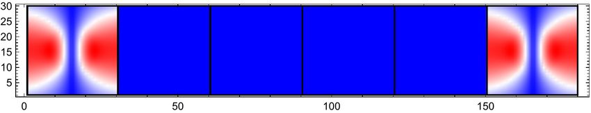
irreducible representation E. To revise this point more clearly, the specific fields corresponding to the
Frontiers 11R. M. Geilhufe & W. Hergert GTPack: A Mathematica group theory package
The point group of the square lattice is C 4 v. c4vct contains the character table of the group.
Read the 2nd eigenmode at M and analyze.
= [
{ - - }
! ! " # ]$
%& & [ [[ ]] ' !( ! #
! % & ) ]
- - - -
× × × ×
Read the 3rd eigenmode at M and analyze.
= [
{ - - }
! ! " # ]$
%& & [ [[ ]] ' !( ! #
! % & ) ]
- - - -
× × × ×
Figure 9. Application of the character projection operator to the field corresponding to the degeneracy
between the second and third band of the transversal magnetic mode at M .
modes can be imported into the Mathematica notebook using GTPhMPBFields. Afterwards, the field is
analyzed by applying the character projection operator for each irreducible representation. As expected,
only the application of the operator corresponding to E shows non-zero results, as can be seen in Figure
9.
ADVANTAGES AND LIMITATIONS
As an additional package to the standard Mathematica framework, GTPack is embedded into the
Mathematica framework. The new modules provided within GTPack are designed for application in solid
state physics and photonics and use notations which are common in these research communities. Having
a programming framework at hand comes with the advantage of easy automation which is in contrast
to recently published group theory tables. Most of the provided modules are kept general and can be
applied in connection to any set of matrices forming a group. This allows for applications way beyond the
provided point and space group setup. As usual, the package is constructed in a modular form and can be
extended easily.
GTPack is under ongoing development and therefore comes with limitations in the first version. Among
others, these comprise of the calculation of character tables for space groups and groups containing anti-
unitary symmetry elements. The implemented modules for the calculation of photonic band structures
currently do not reach the same performance as specialized numeric implementations such as MPB. Thus,
export and import modules connect MPB with GTPack. Additionally, modules to export analytically
generated tight-binding Hamiltonians to Fortran help to generate more efficient numeric codes. An
extension to a parallel implementation for the usage of the cluster version of Mathematica is currently
not planned. Concerning the symmetry analysis, irreducible representations can currently only be
12R. M. Geilhufe & W. Hergert GTPack: A Mathematica group theory package associated to the calculated bands if symmorphic space groups are taken into account. An extension for non-symmorphic groups is under development. CONCLUSION We presented the Mathematica group theory package GTPack together with four basic examples. The package contains about 200 additional commands dealing with basic group theory and representation theory and providing tools for applications in solid state physics and photonics. The package itself is structured into several subpackages. In connection to external databases it is possible to load, change and save data, like structural information or parameters for electronic and photonic band structure calculations. The package works externally with a symbolic representation of symmetry elements. Internally, matrices are used. GTPack can be obtained online via the web page http://GTPack.org. ACKNOWLEDGMENTS The authors acknowledge the support of Sebastian Schenk, especially with respect to his help in building up a documentation within the Mathematica framework. Furthermore, we are grateful for discussions and contributions from Markus Däne, Christian Matyssek, Stefan Thomas, Martin Hoffmann, and Arthur Ernst. This publication was funded by the German Research Foundation within the Collaborative Research Centre 762 (projects A4 and B1). Additionally, RMG acknowledges funding from the European Research Council under the European Union’s Seventh Framework Program (FP/2207-2013)/ERC Grant Agreement No. DM-321031. SUPPLEMENTARY MATERIAL The supplementary material comprises of a complete list of implemented modules. Each table from Table 1 to Table 13 contains the respective modules of one subpackage (see main text Fig. 1). The tables contain the name of the module, a short and general explanation and in some cases (when appropriate) a reference to the implemented algorithm or to further information. Auxiliary.m Table 1 Modules of the subpackage Auxiliary.m. The package contains additional modules which were needed for GTPack but which were not covered in the standard Mathematica language. Name Functionality Ref. GTBlueRed defines the color scheme for tables printed within GTPack GTCartesianSphericalHarmonicY calculates spherical harmonics Ylm in Cartesian form GTCartesianTesseralHarmonicY calculates tesseral harmonics Slm in Cartesian form GTClusterFilter removes certain atoms from a given cluster GTCompactStore stores sparse matrices in compact form GTDiracMatrix gives the Dirac matrices Γ̂i in various representations GTEulerAnglesQ checks if an input is a set of Euler angles GTFermiSurfaceXSF calculates the band structure and stores results to XSF file GTGauntCoefficient calculates the Gaunt coefficients Frontiers 13
R. M. Geilhufe & W. Hergert                         GTPack: A Mathematica group theory package

 GTGroupConnection                     plots a graph illustrating the connection between several
                                       groups
 GTGroupHierarchy                      plots a graph illustrating all subgroups of a group
 GTNeighborPlot                        present information about input data to construct adjacency
                                       matrices
 GTPointGroups                         illustrates the subgroup relationships of the 32 point groups
 GTQAbs                                calculates the absolute value of a quaternion
 GTQConjugate                          calculates the conjugate of a quaternion
 GTQInverse                            calculates the inverse of a quaternion
 GTQMultiplication                     multiplies two quaternions
 GTQPolar                              calculates the polar angle of a quaternion
 GTQuaternionQ                         checks if an input is a quaternion
 GTReadFromFile                        reads an object from a file
 GTSetTableColors                      defines a color function based on the MPB color code
 GTSU2Matrix                           calculates a SU(2) matrix from a given angle and 3D vector
 GTSymbolQ                             checks if an input is a GTPack symbol
 GTTesseralHarmonicY                   calculates tesseral harmonics Slm                             [61]
 GTWriteToFile                         writes an object to a file

Basic.m

Table 2 Modules of the subpackage Basic.m. The package contains modules for basic group theory, like
  calculation of classes, multiplication tables, cosets, etc..

  Name                            Functionality                                               Ref.
  GTAbelianQ                      checks if list of elements forms an Abelian group
  GTAllSymbols                    gives a listed of all currently installed symmetry elements
  GTCenter                        calculates the center of a group
  GTClasses                       calculates the classes of a group
  GTClassMult                     calculates the class multiplication of two classes
  GTClassMultTable                calculates a class multiplication table
  GTConjugacyClass                constructs all conjugate subgroups for a given group and
                                  subgroup
  GTConjugateElement              calculates the conjugate element of an element
  GTCyclicQ                       checks if list of elements forms a cyclic group
  GTGenerators                    estimates a set of generators of a group
  GTGetEulerAngles                gives the Euler angles associated with a symmetry element
  GTGetMatrix                     gives the matrix associated with a symmetry element
  GTGetQuaternion                 gives the quaternion associated with a symmetry element
  GTGetRotationMatrix             gives the 3D rotation matrix associated with a symmetry
                                  element
  GTGetSU2Matrix                  gives the SU(2) matrix associated with a symmetry element
  GTGetSubGroups                  calculates the subgroups of a given group
  GTGetSymbol                     gives the symbol associated with a symmetry element
  GTgmat                          group multiplication
  GTGroupOrder                    calculates the order of a group

                                                                                                     14
R. M. Geilhufe & W. Hergert GTPack: A Mathematica group theory package
GTGroupQ checks if list of elements forms a group
GTInverseElement calculates the inverse of a symmetry element
GTInvSubGroupQ checks if one group is an invariant subgroup of another one
GTInvSubGroups calculates the invariant subgroups of a given group
GTLeftCosets constructs left cosets for a given group and subgroup
GTMagnetic logical module to allow for magnetic groups
GTMagneticQ checks if magnetic groups are considered
GTMultTable calculates the multiplication table of a group
GTNormalizer calculates the normalizer of a group
GTOrderOfElement calculates the order of a symmetry element
GTProductGroup constructs the product group of two groups
GTProductGroupQ checks if a group is a product of two given groups
GTQuotientGroup constructs the quotient group of two groups
GTQuotientGroupQ checks if two groups can form a quotient group
GTRightCosets constructs right cosets for a given group and subgroup
GTSelfAdjointQ checks if a symmetry element is self-adjoint
GTSetMultiplication multiplies the elements of two sets with each other
GTSubGroupQ checks if one group is a subgroup of another one
GTTransformation applies a transformation operator to a given vector
GTTransformationOperator applies a transformation operator to a given vector
GTType gives a symmetry element in space group form
GTWhichInput checks if the input is a symbol, matrix, quaternion or set of
angles
GTWhichOutput transforms an output to a symbol, matrix, quaternion or set
of angles
CrystalField.m
Table 3 Modules of the subpackage CrystalField.m. The package contains modules needed within
crystal field theory, like calculation of the crystal field Hamiltonian, crystal field operators and crystal
field parameters.
Name Functionality Ref.
GTBSTOperator calculates a matrix for Buckmaster-Smith-Thornley [33]
operator equivalent
GTBSTOperatorElement calculates matrix elements for Buckmaster-Smith-Thornley [33]
operator equivalents
GTCFDatabaseInfo gives a list of stored rl expectation values
GTCFDatabaseRetrieve retrieves stored rl expectation values from a file
GTCFDatabaseUpdate adds rl expectation values to a file
GTCrystalField calculates an effective crystal field Hamiltonian
GTCrystalFieldParameter calculates crystal field parameters in the point-charge model
GTCrystalFieldSplitting calculates the decomposition of irreducible representations
within a subgroup
GTStevensOperator calculates a matrix for Stevens operator equivalent [62]
GTStevensOperatorElement calculates matrix elements for Stevens operator equivalents [62]
Frontiers 15R. M. Geilhufe & W. Hergert GTPack: A Mathematica group theory package
GTStevensTheta gives multiplet prefactors for the crystal field expansion [? ]
CrystalStructure.m
Table 4 Modules of the subpackage CrystalStructure.m. The package contains modules for the handling
of crystal structures and crystal structure databases.
Name Functionality Ref.
GTAllStructures prints a list of currently installed structures
GTBravaisLattice gives lattice vectors for a specified crystal system
GTBuckyBall gives a cluster of carbon atoms in buckminsterfullerene
structure
GTClusterManipulate allows for manipulation of atomic clusters
GTCrystalData provides information about crystal structures
GTCrystalSystem gives a list of point groups for a specified crystal system
GTExportXSF exports structures to XC RY SD EN format
GTGetStructure gives an installed crystal structure
GTGroupNotation change notation between Schönflies and Hermann-Mauguin
GTImportCIF imports crystal structure information from CIF files [34]
GTInstallStructure installs new crystal structures
GTLatticeVectors constructs lattice vectors from lattice parameters and angles
GTLoadStructures load stored crystal structures
GTPlotCluster plots a cluster of atoms
GTPlotStructure plots an installed crystal structure
GTPlotStructure2D plots an installed 2D crystal structure
GTSaveStructures saves a set of installed crystal structures
GTShowSymmetryElements plots symmetry elements of a point group
GTSpaceGroups gives information about nomenclature of the 230 space
groups
GTTubeParameters calculates the important geometric properties of single wall
carbon nanotubes
GTTubeStructure constructs a (n, m) single wall carbon nanotube.
ElectronicStructure.m
Table 5 Modules of the subpackage ElectronicStructure.m. The package contains general modules for
electronic structure calculations like calculation of band structures or density of states from various
effective Hamiltonians.
Name Functionality Ref.
GTBands calculates the energy bands for an effective Hamiltonian
GTBandsPlot plots a calculated band structure
GTBandStructure calculates and plots the band structure for an effective
Hamiltonian
GTCompatibility calculates the compatibility relations of two point groups
GTDensityOfStates calculates the density of states for an effective Hamiltonian
GTDensityOfStatesPlot plots a calculated density of states
16R. M. Geilhufe & W. Hergert GTPack: A Mathematica group theory package
GTDensityOfStatesRS calculates the density of states for an effective Hamiltonian
in real space
GTFermiSurface calculates the Fermi-surface
Install.m
Table 6 Modules of the subpackage Install.m. The package contains modules for the installation of
groups and symmetry elements.
Name Functionality Ref.
GTChangeRepresentation changes the standard representation used by GTPack
(SO(3), SO(2), SU(2), ...)
GTGroupFromGenerators installs a finite group from a set of generators
GTInstallAxis installs symmetry elements for a given rotation axis
GTInstallGroup installs point and space groups
GTReinstallAxes changes between active and passive convention for
symmetry elements
GTTableToGroup install a permutation group from the multiplication table
GTWhichAxes informs if active or passive convention for symmetry
elements is used
GTWhichRepresentation gives the currently used standard representation (SO(3),
SO(2), SU(2), ...)
Lattice.m
Table 7 Modules of the subpackage Lattice.m. The package contains modules connected to
crystallographic lattices, like calculation of reciprocal lattice vectors, illustration of Wigner-Seitz cells
and Brillouin zones and the construction of atomic clusters.
Name Functionality Ref.
GTAdjacencyMatrix calculates an adjacency matrix for a cluster of atoms
GTBZLines generates a set of ~k-points for a Brillouin zone path
GTBZMPBPointMesh exports a set of ~k-points in MPB data format [36, 37]
GTBZPath ~
generates a standard k-path in the Brillouin zone
GTBZPointMesh gives a ~k-point mesh in the irreducible part of the Brillouin
zone
GTCluster constructs a spherical cluster of atoms
GTGroupOfK calculates the group of the wave-vector ~k
GTLatCluster constructs a spherical cluster of lattice points
GTLatShells separates a cluster of lattice points into distinct shells
GTReciprocalBasis calculates the reciprocal basis
GTShells separates a cluster of atoms into distinct shells
GTStarOfK calculates the star of the wave-vector ~k
GTVoronoiCell plots the Brillouin zone or Wigner-Seitz cell
Frontiers 17R. M. Geilhufe & W. Hergert GTPack: A Mathematica group theory package
Molecules.m
Table 8 Modules of the subpackage Molecules.m. The package contains modules for the handling of
molecules and molecule structure databases.
Name Functionality Ref.
GTMolChemicalData gives molecular data from the Mathematica database in
GTPack form
GTMolDatabaseInfo gives information of molecular data stored within a database
GTMolDatabaseUpdate add molecular information to a database
GTMolGetMolecule gives information of a particular molecule stored within a
database
GTMolPermutationRep gives a representation of a group in terms of permutation
matrices
GTMolToCluster transforms a molecule from a data set into a cluster of atoms
Photonics.m
Table 9 Modules of the subpackage Photonics.m. The package contains modules for the study of
photonic crystals.
Name Functionality Ref.
GTPhBandsObjects
GTPhCuboid gives the structure factor for a cuboid
GTPhDCObjects calculates the Fourier transform of the inverse permittivity
of a set of geometric objects
GTPhDCPixel calculates the Fourier transform of the inverse permittivity
defined by a pixel map
GTPhDielectric calculates the Fourier transform of −1 (~r)
GTPhEllipticRod gives the structure factor of an elliptic rod
GTPhFields calculates the electro magnetic field in a photonic crystal
GTPhMaster constructs the master equation for a photonic crystal [24]
structure
GTPhMasterObjects constructs the master equation from a list of objects [24]
GTPhMasterPixel constructs the master equation if the permittivity is given by
a pixelmap
GTPhMPBBands imports a photonic band structure calculated by MPB [36, 37]
GTPhMPBFields imports electromagnetic field components calculated with [36, 37]
MPB
GTPhPermittivity ~ for all reciprocal lattice vectors used in the
gives −1 (G)
master equation
GTPhPixelSmooth gives a smoothed pixel map
GTPhPixelStructure allows to perform a modification of the permittivity
distribution defined by a pixel map
GTPhPrismaticRod gives the structure factor of a prismatic rod
GTPhRodSmooth gives a smoothed structure factor of a rectangular rod
18R. M. Geilhufe & W. Hergert GTPack: A Mathematica group theory package
GTPhShowStructure plots an image of the arrangement of dielectric objects in a
photonic structure
GTPhSlab gives the structure factor of a slab
GTPhSlabSmooth gives a smoothed structure factor of a slab
GTPhSphere gives the structure factor of a sphere
GTPhSymmetryBands performs a symmetry analysis of electromagnetic fields for [24]
a given band structure
GTPhSymmetryField performs the symmetry analysis of an electromagnetic field
GTPhSymmetryPoint performs the symmetry analysis of electromagnetic fields
given in datasets
PseudoPotential.m
Table 10 Modules of the subpackage PseudoPotential.m. The package contains modules for the
construction of plane-wave Hamiltonians.
Name Functionality Ref.
GTPwDatabaseInfo gives information about the pseudopotential parameter sets
stored in a database
GTPwDatabaseRetrieve retrieves pseudopotential parameter sets stored in a database
GTPwDatabaseUpdate adds pseudopotential parameter sets to a database
GTPwDielectricF defines a screening function
GTPwEmptyLatticeIrep determines the irreducible representations of the empty
lattice band structure
GTPwHamiltonian constructs a Hamiltonian based on pseudopotential theory [44, 45]
GTPwPrintParmSet prints a parameter set form a pseudopotential database
RepresentationTheory.m
Table 11 Modules of the subpackage RepresentationTheory.m. The package contains modules for basic
representation theory, like calculation of character tables and installation and handling of irreducible
representations.
Name Functionality Ref.
GTAngularMomentumChars gives characters of a matrix representation in terms of
Wigner D-matrices
GTAngularMomentumRep gives a matrix representation in terms of Wigner D-matrices
GTCharacterTable calculates the character table [41]
GTCharProjectionOperator applies the character projection operator to a given function
GTClebschGordanCoefficients calculation of Clebsch Gordan coefficients [43]
GTClebschGordanSum calculates the Clebsch-Gordan sum (direct sum) of two
representation
GTClebschGordanTable illustrates calculated Clebsch-Gordan coefficients
GTDirectProductChars calculates characters of a direct product representation
GTDirectProductRep calculates matrices of a direct product representation
GTExtraRepresentations calculates the extra representations within a double group
Frontiers 19R. M. Geilhufe & W. Hergert GTPack: A Mathematica group theory package
GTGetIrep calculates matrices of irreducible representations [42]
GTIrep calculates the number of times an irred. rep. occurs within
a red. rep.
GTIrepDimension calculates the dimensions of the irreducible representations
GTNumberOfIreps calculates the number of inequivalent irreducible
representations
GTProjectionOperator applies the projection operator to a given function
GTReality estimates if a representation is potentially real, essentially
complex or pseudo-real
GTRegularRepresentation calculates the regular representation of a group
GTSOCSplitting calculates the splitting of states due to spin-orbit coupling
GTSpinCharacters calculates the characters of the spin representation
GTWignerProjectionOperator applies the projection operator to spherical harmonics
TightBinding.m
Table 12 Modules of the subpackage TightBinding.m. The package contains modules for the
construction of tight-binding Hamiltonians in two- and three-center form.
Name Functionality Ref.
GTFindStateNumbers findes the number of states within a certain energy interval
(real space)
GTHamiltonianPlot illustrates zero and non-zero entries within the tight-binding
Hamiltonian
GTPlotStateWeights plots the contribution of atomic sites to an electronic state
(real space)
GTSymmetryBasisFunctions calculates the associated irreducible representation of a
wave function
GTTbAtomicWaveFunction calculates values of an atomic-like wave function
GTTbDatabaseInfo gives information about tight-binding parameters stored in [63]
a database
GTTbDatabaseRetrieve retrieves tight-binding parameters from a database
GTTbDatabaseUpdate adds tight-binding parameters to a database
GTTbGetParameter gives a particular tight-binding parameter from a database
GTTbHamiltonian constructs a tight-binding Hamiltonian [46]
GTTbHamiltonianElement constructs a single element of a tight-binding Hamiltonian
GTTbHamiltonianRS constructs a real space tight-binding Hamiltonian
GTTbNumberOfIntegrals calculates the number of independent tight-binding [47]
integrals
GTTbParameterNames creates a set of parameter names
GTTbParmToRule gives a rule to replace tight-binding symbols using a given
parameter set
GTTbPrintParmSet prints a tight-binding parameter set from a database
GTTbRealSpaceMatrix constructs the interaction of two atoms in a tight-binding
Hamiltonian
GTTbSpinMatrix gives elementary spin matrices for tight-binding [61]
Hamiltonians
20R. M. Geilhufe & W. Hergert GTPack: A Mathematica group theory package
GTTbSpinOrbit adds spin-orbit coupling to a given tight-binding
Hamiltonian
GTTbSymbol2C gives a symbol according to the nomenclature of the two-
center approximation
GTTbSymmetryBandStructure performs a symmetry analysis of a given band structure
GTTbSymmetryPoint performs a symmetry analysis of energy bands at a specified
~k-point
GTTbSymmetrySingleBand performs a symmetry analysis of a single energy band
GTTbToFortran transforms a k-space tight-binding Hamiltonian into a
FORTRAN module
GTTbToFortranList prints a Hamiltonian as FORTRAN code
GTTbWaveFunction constructs a tight-binding wave-function
Vibrations.m
Table 13 Modules of the subpackage Vibrations.m. The package contains modules for the study of
vibrational modes of solids and molecules.
Name Functionality Ref.
GTVibDisplacementRep gives the displacement representation of a molecule
GTVibDynamicalMatrix gives the dynamical matrix for a given structure
GTVibModeSymmetry gives the vibrational modes of a molecule
GTVibSetParameters substitutes spring constants and masses within a dynamical
matrix
GTVibTbToPhonon transforms a tight-binding p-Hamiltonian into a dynamical [64]
matrix
GTVibTbToPhononRule gives rules to transform a tight-pinding p-Hamiltonian into
a dynamical matrix
REFERENCES
[1] Wigner E. Fifty years of symmetry operators. Understanding the Fundamental Constituents of
Matter (Springer) (1978), 879–892.
[2] Ahmad S, International Centre for Theoretical Physics TI. Group theory, the new language of modern
physics. Tech. rep., International Centre for Theoretical Physics (1990).
[3] Bouckaert LP, Smoluchowski R, Wigner E. Theory of brillouin zones and symmetry properties of
wave functions in crystals. Physical Review 50 (1936) 58–67. doi:10.1103/PhysRev.50.58.
[4] Bethe HA. Splitting of terms in crystals. Annalen der Physik 3 (1929) 133.
[5] Inui T, Uemura Y. Theory of color centers in ionic crystals i electronic states of f-centers in alkali
halides. Progress of Theoretical Physics 5 (1950) 252–265.
[6] Chanier T, Opahle I, Sargolzaei M, Hayn R, Lannoo M. Magnetic state around cation vacancies in
ii–vi semiconductors. Physical review letters 100 (2008) 026405.
[7] Bassani F, Parravicini GP. Electronic states ans optical transitions in solids (Pergamon Press) (1975).
[8] Miyamachi T, Schuh T, Märkl T, Bresch C, Balashov T, Stöhr A, et al. Stabilizing the magnetic
moment of single holmium atoms by symmetry. Nature 503 (2013) 242–246.
Frontiers 21R. M. Geilhufe & W. Hergert GTPack: A Mathematica group theory package
[9] König A, Mermin ND. Screw rotations and glide mirrors: Crystallography in fourier space.
Proceedings of the National Academy of Sciences 96 (1999) 3502–3506.
[10] Liu CX, Qi XL, Zhang H, Dai X, Fang Z, Zhang SC. Model hamiltonian for topological insulators.
Physical Review B 82 (2010) 045122. doi:10.1103/PhysRevB.82.045122.
[11] Volovik GE, Gor’kov LP. Superconducting classes in heavy-fermion systems. Ten Years of
Superconductivity: 1980–1990 (Springer) (1985), 144–155.
[12] Blount EI. Symmetry properties of triplet superconductors. Physical Review B 32 (1985) 2935.
[13] Sigrist M, Ueda K. Phenomenological theory of unconventional superconductivity. Reviews of
Modern Physics 63 (1991) 239.
[14] Geilhufe RM, Balatsky AV. Symmetry analysis of odd-and even-frequency superconducting gap
symmetries for time-reversal symmetric interactions. Physical Review B 97 (2018) 024507.
[15] Fernandes RM, Orth PP, Schmalian J. Intertwined vestigial order in quantum materials: nematicity
and beyond. arXiv preprint arXiv:1804.00818 (2018).
[16] Bradlyn B, Elcoro L, Cano J, Vergniory MG, Wang Z, Felser C, et al. Topological quantum chemistry.
Nature 547 (2017) 298 EP –. Article.
[17] Geilhufe RM, Bouhon A, Borysov SS, Balatsky AV. Three-dimensional organic dirac-line materials
due to nonsymmorphic symmetry: A data mining approach. Physical Review B 95 (2017) 041103.
[18] Geilhufe RM, Borysov SS, Bouhon A, Balatsky AV. Data mining for three-dimensional organic dirac
materials: Focus on space group 19. Scientific reports 7 (2017) 7298.
[19] Wieder BJ, Kane CL. Spin-orbit semimetals in the layer groups. Physical Review B 94 (2016)
155108. doi:10.1103/PhysRevB.94.155108.
[20] Bouhon A, Black-Schaffer AM. Global band topology of simple and double dirac-point semimetals.
Physical Review B 95 (2017) 241101.
[21] Nayak C, Simon SH, Stern A, Freedman M, Sarma SD. Non-abelian anyons and topological quantum
computation. Reviews of Modern Physics 80 (2008) 1083.
[22] López-Tejeira F, Ochiai T, Sakoda K, Sánchez-Dehesa J. Symmetry characterization of eigenstates
in opal-based photonic crystals. Physical Review B 65 (2002) 195110.
[23] Hergert W, Däne M. Group theoretical investigations of photonic band structures. physica status
solidi (a) 197 (2003) 620–634.
[24] Sakoda K. Optical properties of photonic crystals, vol. 80 (Springer Science & Business Media)
(2004).
[25] Sakoda K, Shiroma H. Numerical method for localized defect modes in photonic lattices. Physical
Review B 56 (1997) 4830.
[26] Stefanou N, Karathanos V, Modinos A. Scattering of electromagnetic waves by periodic structures.
Journal of Physics: Condensed Matter 4 (1992) 7389.
[27] Sakoda K. Symmetry, degeneracy, and uncoupled modes in two-dimensional photonic lattices.
Physical Review B 52 (1995) 7982.
[28] Altmann S, Herzig P. Point-group theory tables (Oxford University Press) (1994).
[29] Bradley C, Cracknell A. The mathematical theory of symmetry in solids: representation theory for
point groups and space groups (Oxford University Press) (2010).
[30] Aroyo MI, Perez-Mato J, Orobengoa D, Tasci E, De La Flor G, Kirov A. Crystallography online:
Bilbao crystallographic server. Bulg. Chem. Commun 43 (2011) 183–97.
[31] GAP. GAP – Groups, Algorithms, and Programming, Version 4.8.5. The GAP Group (2016).
[32] Hergert W, Geilhufe M. Group Theory in Solid State Physics and Photonics. Problem Solving with
Mathematica (Wiley-VCH) (2018).
22You can also read