Infinitely Many Multipulse Solitons of Different Symmetry Types in the Nonlinear Schr odinger Equation with Quartic Dispersion
←
→
Page content transcription
If your browser does not render page correctly, please read the page content below
Infinitely Many Multipulse Solitons of Different Symmetry Types
                                                 in the Nonlinear Schrödinger Equation with Quartic Dispersion
                                               Ravindra Bandara∗1,3 , Andrus Giraldo1,3 , Neil G. R. Broderick2,3 , and Bernd Krauskopf1,3
                                                  1
                                                      Department of Mathematics, University of Auckland, Auckland 1010, New Zealand.
                                                        2
                                                          Department of Physics, University of Auckland, Auckland 1010, New Zealand.
                                                       3
                                                         The Dodd-Walls Centre for Photonic and Quantum Technologies, New Zealand.

                                                                                               March 31, 2021
arXiv:2103.16053v1 [nlin.PS] 30 Mar 2021

                                                                                                    Abstract
                                                      We show that the generalised nonlinear Schrödinger equation (GNLSE) with quartic dispersion supports
                                                  infinitely many multipulse solitons for a wide parameter range of the dispersion terms. These solitons exist
                                                  through the balance between the quartic and quadratic dispersions with the Kerr nonlinearity, and they
                                                  come in infinite families with different signatures. A travelling wave ansatz, where the optical pulse does not
                                                  undergo a change in shape while propagating, allows us to transform the GNLSE into a fourth-order nonlinear
                                                  Hamiltonian ordinary differential equation with two reversibilities. Studying families of connecting orbits
                                                  with different symmetry properties of this reduced system, connecting equilibria to themselves or to periodic
                                                  solutions, provides the key to understanding the overall structure of solitons of the GNLSE. Integrating a
                                                  perturbation of them as solutions of the GNLSE suggests that some of these solitons may be observable
                                                  experimentally in photonic crystal wave-guides over several dispersion lengths.

                                           1      INTRODUCTION
                                           Recently, Blanco-Redondo et al. experimentally discovered pure quartic solitons (PQS) in a silicon photonic
                                           crystal waveguide [5]. Such PQS exist due to a balance between negative quartic dispersion and the Kerr
                                           nonlinearity — unlike conventional optical solitons which balance quadratic dispersion and nonlinearity. This
                                           balance through the quartic dispersion allows for an unusual scaling of the pulse width with the power, which
                                           makes them attractive for short-pulse lasers [5]. Furthermore, these new solitons have decaying oscillating tails.
                                           Pure quartic solitons have been the focus of several recent studies, both experimental and theoretical [35, 36, 37].
                                               It is well known that the generalised nonlinear Schrödinger equation (GNLSE) can be used to model optical
                                           pulse propagation in fibres in a variety of different regimes, including the case of higher-order dispersion. An
                                           analytic solution in the presence of both quartic and quadratic dispersion was found by Karlson and Höök [25]
                                           in the form of a squared hyperbolic secant pulse shape. It exists in the situation when both the quadratic
                                           and the quartic dispersion coefficients, β2 and β4 , are negative. Furthermore, the Karlson and Höök solution
                                           family does not possess oscillating decaying tails; thus, it does not describe PQS. Subsequently, Piché et al. [31]
                                           numerically studied the effect of third-order dispersion together with second and fourth-order dispersion. With
                                           numerical simulations, they found that, when a weak third-order dispersion is introduced, the temporal profile
                                           and the peak power of the soliton remain unchanged. Akhmediev et al. [2] found that, when both β2 and
                                           β4 are negative, solitons have either exponentially decaying tails or oscillating tails, depending on the soliton
                                           propagation constant (nonlinear shift of the wave number). Interaction of solitons with oscillating tails was
                                           numerically studied by Akhmediev and Buryak [3]. They found that the oscillating tails of a soliton establish a
                                           potential barrier between neighbouring solitons during their interactions, preventing two adjacent solitons from
                                           combining. Furthermore, they investigated the bound states of two or more solitons when the single soliton
                                           has oscillating tails [7]. Roy and Biancalana [32] demonstrated that, when both β2 and β4 are negative, it is
                                           possible to observe solitons in silicon-based slot waveguides. Although there have been many studies of solitons
                                           in the presence of both quartic and quadratic dispersions, all these works considered the situation when both
                                           β2 and β4 are negative. More recently Tam et al. [35, 37] considered the case when β4 is negative while β2 can
                                           have either sign. They numerically found that single-hump solitons exist for some positive β2 values as well.
                                           Furthermore, they explained that the decay rate of the solitons decreases as β2 increases.
                                               ∗ ravindra.bandara@auckland.ac.nz

                                                                                                        1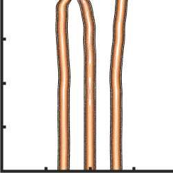
In this paper, we perform a detailed analysis of the GNLSE to find solitons of different types (multi-hump
solitons) with different symmetry properties, beyond the one-hump soliton obtained in [37] and for different
signs of the quadratic dispersion term. By taking a dynamical system approach, we show that the GNLSE
supports infinitely many multi-hump solitons in the presence of both quartic and quadratic dispersion. We
consider the situation when β4 is negative, and show that these multi-hump solitons exist not only when β2
is negative. More specifically, we extend the work in [7] and [37] and present the parameter range for which
these multi-hump solitons also exist when β2 is positive. Moreover, we show that, apart from symmetric and
antisymmetric solitons, there also exist nonsymmetric, symmetry-broken solitons, which are distinct from a
union of fundamental solitons. For fixed negative β4 , we determine the parameter intervals of β2 over which the
different types of solitons exists. This is achieved via a travelling wave ansatz that transforms the GNLSE into a
fourth-order Hamiltonian ordinary differential equation (ODE) with two reversible symmetries. Solitons of the
GNLSE are then identified as homoclinic solutions to the origin of this ODE, which we find and track with state-
of-the art continuation techniques. We discuss a connection of our findings with results obtained, for example,
for the Swift-Hohenberg equation [6] and the Lugiato-Lefeverer equation [30], and demonstrate that the overall
bifurcation structure of the GNLSE can be characterised as truncated homoclinic snaking. Moreover, we show
that connecting orbits from the origin to periodic orbits (also referred to as EtoP connections) with different
symmetry properties organise different infinite families of multi-hump solitons. The structure of periodic orbits
is discussed briefly to show that infinitely many of them create different connections to the origin and, hence,
associated families of solitons. Importantly, our results apply to any negative values of the quartic dispersion
term via a suitable transformation. Finally, we investigate the evolution of these solitons along a waveguide via
the integration of the GNLSE with a split-step Fourier method; here we consider symmetric and non-symmetric
solitons for β2 = 0 and also for different signs of β2 . Our numerical simulations indicate that some of the
multi-hump solitons are only weakly unstable and may propagate effectively unchanged over many dispersion
lengths; hence, they might be observable in careful experiment with currently available waveguides.
    The paper is structured as follows. In Sec. 2, we introduce the GNLSE, and show how it can be transformed
into an ODE; we then discuss the special mathematical properties of this ODE, present its local bifurcation
analysis and also discuss the role of its homoclinic solutions as solitons of the GNLSE. In Sec. 3, we set up
suitable boundary value problems to find and then continue homoclinic solutions, periodic solutions and EtoP
connections. In Sec. 4, we present one-by-one families of homoclinic solutions of different symmetry types, show
over which β2 -range they exist and discuss the connection with homoclinic snaking. Section 5 then shows that
the respective homoclinic solutions occur along parabolas in different parameter planes. In Sec. 6 we show that
there are infinitely many periodic orbits that create families of connecting orbits and, hence, a menagerie of
solitons with different signatures. In Sec. 7, we present some simulations of the GNLSE that demonstrate that,
while only the single-pulse primary soliton is stable, certain multi-hump solitons are only weakly unstable and,
thus, may be observable in an experimental settings. Finally, a discussion of the results and an outlook to future
research are presented in Sec. 8.

2    MATHEMATICAL ANALYSIS
Pulse propagation along an optical fibre under the influence of quadratic dispersion, quartic dispersion and the
Kerr nonlinearity is governed by the GNLSE [1]

                                      ∂A                β2 ∂ 2 A     β4 ∂ 4 A
                                         = iγ|A|2 A − i          + i          .                               (1)
                                      ∂z                2 ∂t2        24 ∂t4
Here, A(z, t) is the slowly varying complex pulse envelope, z is the propagation distance, t is the time in a
co-moving frame of the pulse, γ is the coefficient of the nonlinearity, and β2 and β4 are the quadratic and
quartic dispersion coefficients, respectively. In order to focus on the essential interactions between dispersion
and nonlinearity that drive soliton formation, Eq. (1) does not include losses and higher-order terms such as
the Raman effect.
     We note that it is possible to reduce Eq. (1) to a parameter-free form by using a rescaling transforma-
tion. However, as shown in Table 1, depending on the sign of β2 and β4 , it is necessary to consider different
transformations. That is, each quadrant of the (β2 , β4 )-plane has a corresponding transformation that reduces
Eq. (1) into a parameter-free form. In particular, Akhmediev et al. [2] considered the transformation of case
(d) in Table 1; thus, they considered the situation when both β2 and β4 are negative. Furthermore, all the
transformations are undefined when β2 = 0 or β4 = 0, and there is no continuous transition between different
signs of β2 and β4 . Therefore, none of the reduced PDEs are able to describe the case of PQS. For the purpose
of this paper, we are interested in the transition between β2 < 0, β2 = 0 (PQS) and β2 > 0. Thus, we consider
the original GNLSE without reducing the parameters first. We stress that our results are general because they
can be mapped to any specific parameter region by the corresponding transformations for given signs of β2 and
β4 .

                                                         2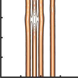
Quadrant Transformation Non-dimensionalised GLNSE
∂U ∂2U ∂4U
(a) β2 > 0, β4 > 0 = i|U |2 U − i 2 + i 4
∂x ∂τ ∂τ
s
sign(β4 )β4 γ 6β22 ∂U ∂2U ∂4U
(b) β2 < 0, β4 > 0 U= A, x = z = i|U |2 U + i 2 + i 4
6β22 sign(β4 )β4 ∂x ∂τ ∂τ
s
12 sign(β2 )β2 ∂U ∂2U ∂4U
(c) β2 > 0, β4 < 0 τ= t = i|U |2 U − i 2 − i 4
sign(β4 )β4 ∂x ∂τ ∂τ
∂U ∂2U ∂4U
(d) β2 < 0, β4 < 0 = i|U |2 U + i 2 − i 4
∂x ∂τ ∂τ
Table 1: Different transformations to reduce the GNLSE to a parameter-free form in each quadrant of the
(β2 , β4 )-plane.
When solving the GNLSE one looks for solutions, where the pulse is stationary and does not change with
propagation distance. We study here such travelling wave solutions of the form
A(z, t) = u(t)eiµz , (2)
where u(t) is the temporal profile of the pulse and µ is the soliton propagation constant (nonlinear shift of the
wavenumber) [2]. Note that the intensity of such solutions, |A(t)|2 = u(t)2 , is unchanged during propagation.
After substituting Eq. (2) into Eq. (1) we obtain the fourth-order nonlinear ODE
β4 d4 u β2 d2 u
− − µu + γu3 = 0. (3)
24 dt4 2 dt2
d2 u d3 u
By introducing the new variables u1 , u2 , u3 and u4 such that u = (u1 , u2 , u3 , u4 ) = u, du ,
dt dt 2 , dt3 , Eq. (3)
can be written as the system of four first-order ODEs
u2
u3
du
u4
= f (u, ζ) = ! , (4)
dt 24 β
2 3
u3 + µu1 − γu1
β4 2
where ζ = (β2 , β4 , γ, µ) ∈ R4 . Note that system (4) is reversible [11] under the transformations
R1 : (u1 , u2 , u3 , u4 ) → (u1 , −u2 , u3 , −u4 ) and
R2 : (u1 , u2 , u3 , u4 ) → (−u1 , u2 , −u3 , u4 ).
This means that if u(t) is a solution then both R1 (u(−t)) and R2 (u(−t)) are also solutions of system (4).
Throughout the paper, we refer to R1 (u(−t)) and R2 (u(−t)) as the R1 - and R2 -counterpart of u(t), respectively.
Furthermore, S = R1 ◦ R2 = R2 ◦ R1 , is the state-space symmetry
S : (u1 , u2 , u3 , u4 ) → (−u1 , −u2 , −u3 , −u4 )
of system (4), which is point reflection in the origin 0. The set of points that are left invariant under R1 or R2
are known as symmetric or reversibility sections of system (4); they are
Σ1 = {u ∈ R4 : u2 = u4 = 0} and
Σ2 = {u ∈ R4 : u1 = u3 = 0},
respectively. Note that the origin 0 is the only point that belongs to both Σ1 and Σ2 , that is, it is the only
point that is invariant under S. A solution trajectory u(t) of system (4) is called symmetric if it satisfies either
R1 (u(−t)) = u(t) or R2 (u(−t)) = u(t). One can show that if u(t) is a symmetric solution, then there exists a
time t∗ ∈ R such that u(t∗ ) ∈ Σ1 or u(t∗ ) ∈ Σ2 , that is, u(t) intersects Σ1 or Σ2 . To distinguish the invariance
3between the two reversibility conditions R1 and R2 , we refer to a solution that is only invariant under R1 as a
R1 -symmetric solutions of system (4), and similarly define R2 -symmetric solutions. Furthermore, if a solution is
invariant under both R1 and R2 , then we refer to it as R∗ -symmetric. Notice that if a solution is R∗ -symmetric,
then it is invariant under S; however, invariance under S does not necessarily imply R∗ -symmetry. Lastly, a
solution that is neither invariant under R1 nor R2 is referred to as non-symmetric.
System (4) can be transformed into the form of a Hamiltonian system by the change of coordinates
p = (p1 , p2 ) = (u2 , u4 ),
−12β2
q = (q1 , q2 ) = u1 + u3 , u1 ,
β4
where p and q are the generalised position and momentum coordinates. With this transformation, system (4)
can be written as
dq1 − 12β2
p1 + p2
dt β4
dq p
2 1
dt 12β ,
= q +
2
q (5)
dp 1 1 2
β4
dt ! !
24 β2 12β
dp2 q1 +
2 3
q2 + µq2 − γq2
β4 2 β4
dt
which satisfies the well-known Hamiltonian equations [11]
dq b
∂H dp b
∂H
= , =− . (6)
dt ∂p dt ∂q
Here the conserved quantity or energy is
2
b 6β2 2 1 12β2
H(p, q) = p1 p2 − p1 + q1 + q2
β4 2 β4
6γq24 − 12µq22
+ , (7)
β4
as obtained from system (5) by integration with respect to p and q. This expression can be written in original
coordinates as
1 6β2 u22 − 6γu41 + 12µu21
H(u) = u2 u4 − u23 − , (8)
2 β4
and it is a conserved quantity along solution trajectories of system (4). We remark that one can also derive
Eq. (8) by using the general expression for fourth-order reversible systems provided in [8]. Notice that, if a
solution trajectory converges backward or forward in time to an equilibrium u0 of system (4) with energy H(u0 ),
then the solution trajectory has energy H(u0 ) for all times.
We now focus our attention on the equilibria of system (4). The origin 0 = (0, 0, 0, 0) is an equilibrium
for
q any parameter
value. It undergoes a pitchfork bifurcation at µ = 0, which creates two equilibria E± =
µ
± γ , 0, 0, 0 for µγ > 0. These are the only equilibria of system (4). Note that 0 ∈ Σ1 ∩ Σ2 , while E± lie
only in Σ1 . Hence, all equilibria are symmetric: 0 is invariant under both R1 and R2 , and E± are invariant
under R1 only. Note from Eq. (8) that, for any choice of the parameters, 0 always lies in the zero energy level.
6µ2
This is not the case for the other two equilibria E± for which H(E± ) = − γβ 4
. Hence, H(E± ) 6= 0 whenever
µ 6= 0 (and β4 , γ 6= 0), so that the equilibria 0 and E± do not lie in the same energy level. Thus, there cannot
be a connecting trajectory between them.
We now focus our attention on homoclinic solutions, which are trajectories of system (4) that converge to the
same equilibrium both forward and backward in time. Homoclinic solutions are sought because they correspond
to solitons of the GNLSE. Since, the solitons of the GNLSE converge to 0, in both forward and backward in
time, we only consider homoclinic solutions to 0 as it is the only equilibrium with u = u1 = 0.
Homoclinic solutions in fourth-order, reversible and Hamiltonian systems have been studied, for example, in
[13, 14, 8, 4, 11, 12, 22]. In particular, results on four-dimensional reversible systems have been developed and
applied in the analysis of a system that describes the dynamics of an elastic strut [8, 4, 12, 11]. It is the case that
symmetric homoclinic solutions in fourth-order reversible systems persist when a suitable parameter is changed
[13, 14, 8]. This is true for both reversible and non-reversible Hamiltonian systems. It has also been proved
4µ (a)
u1 (b)
HH 0.9
1.5
(b) (c) 0
1
u1 (c)
(I) (II) (III) 0.9
0.5
BD 0
−0.75 0 0.75 β2 −5.0 0 5.0 t
Figure 1: Panel (a) shows the bifurcation diagram in the (β2 , µ)- parameter plane for β4 = −1 and γ = 1.
The purple parabola denotes the boundary between the equilibrium 0 having real and complex eigenvalues,
given by BD and HH bifurcation; in the grey shaded region close to the purple parabola, infinitely many
symmetric homoclinic solutions are expected to exist. Panel (b) and (c) show the temporal traces of the
primary homoclinic solution of system (4) for (β2 , β4 , γ, µ) = (−1, −1, 1, 1) and (β2 , β4 , γ, µ) = (0.4, −1, 1, 1), at
the yellow and orange dots in panel (a), respectively.
that each symmetric homoclinic solution in a reversible system is accompanied, for fixed parameter values, by
a one-parameter family of periodic solutions with minimal period T0 . As the period growths to infinity, that
is T0 → ∞, periodic solutions accumulate on a symmetric homoclinic solution. The periodic solutions of these
families lie in different Hamiltonian energy levels, and some of them lie in the energy level with H = 0. As
opposed to the symmetric case, non-symmetric homoclinic solutions in reversible systems do not persist as a
suitable parameter is changed; however, they persist in systems that are both reversible and Hamiltonian [8, 17]
as is the case for system (4). It is a special property of systems that are both reversible and Hamiltonian that
homoclinic solutions persist as codimension-zero phenomena. It has been proven in [12] that a transition of
the equilibrium from a real saddle (spectrum with only real eigenvalues) to a saddle-focus (spectrum with only
complex conjugate eigenvalues), as a parameter is changed, is an organising centre for the creation of infinitely
many symmetric homoclinic solutions, provided the following conditions are satisfied:
(1) the ODE is fourth-order, reversible and Hamiltonian,
(2) there exists a symmetric homoclinic solution at the moment of the transition of the equilibrium.
One refers to this transition as the Belyakov-Devaney (BD) bifurcation [13, 30, 8, 20]. To see whether the second
condition is satisfied for system (4), we first focus our attention on the eigenvalues of its equilibria in different
parameter regimes. The eigenvalues of the linearisation around a symmetric equilibrium of a reversible system
have generically one of the following forms [11]:
(I) two eigenvalues are ±λ1 and the other two are ±λ2 , where λ1 , λ2 ∈ R;
(II) two eigenvalues are ±λ and the other two are ±λ∗ , where λ ∈ C with Re(λ) 6= 0 and Im(λ) 6= 0;
(III) two eigenvalues are ±iλ1 and the other two are ±iλ2 , where λ1 , λ2 ∈ R;
(IV) two eigenvalues are ±λ1 and the other two are ±iλ2 , where λ1 , λ2 ∈ R.
For system (4), one can obtain an analytical expression for the eigenvalues of the linearisation around 0 and
E± . The eigenvalues of 0 are given by [37, 8]:
s !
2 6β2 2β4
λ0 = 1± 1+ 2µ , (9)
β4 3β2
while the eigenvalues of E± are given by
s !
6β2 4β4
λ2E± = 1± 1 − 2µ . (10)
β4 3β2
Since we are interested in homoclinic solutions to 0, we focus our attention on Eq. (9). Notice that the
expression inside the square root defines a parabola in the (β2 , µ)-plane that separates the different cases of
the spectrum of the equilibrium 0. This parabola is shown in Fig. 1(a) as a purple curve that separates the
(β2 , µ)-plane into three regions, where the eigenvalues of 0 are of the form (I), (II) and (III), respectively. Note
that 0 is a real saddle in region (I) and a saddle-focus in region (II). Due to the real eigenvalues of 0, homoclinic
solutions in region (I) must have non-oscillatory exponentially decaying tails. In contrast, homoclinic solutions
5in region (II) must have oscillatory decaying tails because the eigenvalues of 0 are complex conjugates. In the
following sections up to Sec. V, we present our results on the existence of homoclinic solutions for the horizontal
line µ = 1 in (β2 , µ)-plane. This choice of µ-value does not restrict the generality of our results as we will show
in Sec. V; indeed, our results extend throughout the upper half of the (β2 , µ)-parameter plane, that is, when
µ > 0. Figure 1(b) and (c) show two homoclinic solutions along this horizontal line for two distinct β2 -values in
region (I) and (II), respectively. The homoclinic solution in Fig. 1(b) has non-oscillating exponentially decaying
tails as it belongs to region (I). Furthermore, this homoclinic solution persist until β2 reachs the right-hand side
of the parabola in Fig. 1(a), that is, at the boundary between regions (II) and (III) – which correspond to a
Hamiltonian-Hopf (HH) bifurcation [20, 24]. In Fig. 1(c), we show what this homoclinic solution looks like at
β2 = 0.4 where it has oscillating tails. In particular, this homoclinic solution is R1 -symmetric and we refer to it
as the primary homoclinic solution; its corresponding soliton is the one Tam et al considered in [35]. Note that
the homoclinic solution in Fig. 1(c) has oscillatory decaying tails but the oscillations damp out very quickly.
The oscillations in the tails of the these homoclinic solutions increase when moving horizontally towards HH
bifurcation. Because the primary homoclinic solution exists at the transition between regions (I) and (II), the
conditions for a BD bifurcation are satisfied and infinitely many homoclinic solutions must exist in the indicated
grey shaded region near the branch BD in Fig. 1(a)[12].
3 NUMERICAL IDENTIFICATION AND CONTINUATION OF
HOMOCLINIC SOLUTIONS
The task is now to find and identify a representative number of symmetric and non-symmetric homoclinic
solutions of system (4). To this end, we make use of continuation algorithms for two-point boundary value
problems (2PBVP), implemented in the software package Auto-07p [15] and its extension HomCont [10]. In
the 2PBVP formulation, time is rescaled to the interval [0, 1]. Thus, the integration time is treated as a free
parameter that multiplies the right-hand side of system (4), that is,
dv
= T f (v, ζ). (11)
dt
Note that we always assume that T > 0. Suitable boundary conditions are imposed at the starting point v(0)
and the end point v(1) of the solution segment [26]. For the continuation of a homoclinic solution, we use
projection boundary conditions that place v(0) in the unstable eigenspace Eu (0) of the equilibrium 0, and
v(1) in one of the reversibility sections Σ1 or Σ2 . In this way, we take advantage of the reversibility of system
(4) to compute only half of a symmetric homoclinic solution v(t). Convergence forward in time to the stable
eigenspace Es (0) is guaranteed by the corresponding reversibility conditions, and the remaining part of the
homoclinic solution is obtained by applying R1 (v(−t)) or R2 (v(−t)). Notice that this formulation is only able
to continue symmetric homoclinic solutions, since an intersection with a reversibility section is required.
For the case of non-symmetric homoclinic solutions we formulate a 2PBVP of the entire homoclinic solution.
Auto-07P is a general-purpose continuation package designed for generic vector fields, and particular con-
siderations have to be taken when continuing homoclinic and periodic solutions in reversible and Hamiltonian
systems [19]. To deal with the fact that homoclinic solutions generically persist when a single parameter is
varied, we follow [19] and introduce the gradient of the conserved quantity H as a perturbation of the vector
field equations
dv
= T f (v, ζ) + δ∇H, (12)
dt
where δ is an additional continuation parameter. We then impose the boundary conditions that v(0) lies in
Eu (0) and v(1) lies in Es (0). We continue the solution of the overall 2PBVP in one of the parameters while
allowing δ and T to vary. In this setup, the new parameter δ is free but remains extremely close to zero during
continuation [19, 16, 28]. Note that the 2PBVP formulation of the entire homoclinic solution can be used to
continue symmetric homoclinic solutions as well.
To find the first homoclinic solution, we make use of a numerical implementation of Lin’s method [27],
where we consider two orbit segments va (t), vb (t) and a suitable three-dimensional hyperplane Σ. Here, va (0)
and vb (1) lie in Eu (0) and Es (0), respectively, and va (1) and vb (0) both lie in Σ. Then the signed difference
(called the Lin gap) between va (1) and vb (0), along a fixed one-dimensional direction, provides a well-defined
test function whose zeros correspond to homoclinic solutions of system (4); see [27]. Once a zero is found, the
associated homoclinic solution can be followed in system parameters with the previously constructed 2PBVP
formulations. Lin’s method allows us to compute multi-hump homoclinic solutions of different types. We
remark that the Auto demo rev [15], for the GNLSE as considered in [23], contain a setup to continue the basic
homoclinic solutions. However, we are interested in many different types of homoclinic solutions that cannot
be computed from the demo, and they are all identified with Lin’s method.
6Connections between the equilibrium 0 and periodic solutions, which we refer to as EtoP connections, are
organising centres for the existence of homoclinic solutions under mild conditions [29, 9]; hence, they are an
important object to consider when studying homoclinic solutions. To compute EtoP connections, we have to
find first periodic solutions of system (4) that support a connection to 0. In reversible and Hamiltonian systems,
periodic solutions are not isolated in phase space for fixed parameter values [19]. To be able to compute and
continue them, we consider the perturbed system (12) and use the 2PBVP formulation for periodic solutions
[26]. For the initial data of the formulation, we use homoclinic solutions previously constructed with the 2PBVP
above, as they are good initial approximation of periodic solutions of high period. Performing a continuation
step in δ and T allows us to find the family of periodic solutions for fixed parameter values, while δ again
remains practically 0. These solution families form two-dimensional surfaces in phase space where each periodic
solution lies in a particular energy level. Among these solution families, we focus on saddle periodic solutions
in the zero energy level because they are the only periodic solutions that can have connections with 0.
To find connections from 0 to a saddle periodic solution we can follow the approach that we used to find
homoclinic solutions to 0. This requires one to compute first the Floquet multipliers and Floquet bundles of the
periodic solution, as they contain the linear information of the flow near the periodic solution. Saddle periodic
solutions of system (4) have one stable (inside the unit circle) and one unstable (outside of the unit circle)
Floquet multipliers with associated stable and unstable Floquet bundles, respectively. The stable (unstable)
bundle consists of the directions in phase space, along which solutions converge forward (backward) in time to
the periodic solution. Finally, the other two Floquet multipliers of a saddle-periodic solution in system (4) are
always equal to one. Associated to them, there are two Floquet bundles: one that is pointing in the direction
of the flow along the periodic solution, called the trivial bundle, and another one tangent to the surface of the
periodic solutions in phase space.
We compute the Floquet multipliers and their corresponding bundles with a homotopy step for a suitable
2PBVP formulation; see [18] for more details. Note that any connection that converges backward in time to 0
and forward in time to a R1 -symmetric (R2 -symmetric) periodic solution has a R1 -counterpart (R2 -counterpart)
that converges backward in time to the same periodic solution and forward in time to 0. As we are interested
in periodic solutions that are R1 -symmetric or R2 -symmetric, we make use of this fact to set up Lin’s method
by using the unstable eigenspace Eu (0) of 0 and the stable bundle of the periodic solution. That is, we consider
two orbits segments va (t), vb (t) and a suitable three-dimensional hyper plane Σ, such that, va (0) and vb (1) lie
in Eu (0) and the stable Floquet bundle of the saddle periodic solution, respectively, and va (1) and vb (0) lie in
Σ. The zeros of the corresponding Lin gap correspond to EtoP connections that converge backwards in time to
0 and forward in time to the periodic solution.
4 HOMOCLINIC FAMILIES OF DIFFERENT TYPES
Computing EtoP connections between 0 and saddle periodic solutions in the zero-energy level is a good starting
point for understanding how different homoclinic solutions are organised. Since system (4) is reversible, existence
of a connection from 0 to a symmetric saddle periodic solution guarantees a return connection from the periodic
solutions to 0 as well. This return connection corresponds to the R1 - or R2 -counterpart of the EtoP connection,
depending on the symmetry of the periodic solution. The existence of a connection from 0 to a periodic
solution and a connection back from the periodic solution to 0 is known as a heteroclinic cycle. Existence of
these heteroclinic cycles, and their persistence under parameter variation (transversality), generate a mechanism
for the existence of homoclinic solutions that go around the periodic solution multiple times, as a consequence
of the λ-lemma [38, 29]. Thus, it is possible to find homoclinic solutions that
(a) follow closely an EtoP connection from 0 to the periodic solution,
(b) then loop n-times close to the periodic solution, and
(c) follow closely an EtoP connection from the periodic solution back to 0.
The different combinations of EtoP connections generate cycles with different symmetry properties that
organise specific homoclinic solution families in parameter space. Some of these families are organised by EtoP
connections to a R∗ -symmetric periodic solution, and others by EtoP connections to a R1 -symmetric periodic
solution. The corresponding solitons associated with these homoclinic families are distinct from bound states
of two or more primary solitons since the spacing of the maxima is fixed and different from the location of the
zeros of the oscillating tails. In what follows, we study different families of such homoclinic solutions. We show
bifurcation diagrams in β2 of these families to illustrate how they persist and coalesce due to the existence of
different underlying EtoP connections.
7u1 • ×
0.8
0
−0.8
(a1) (a2)
−15 0 15 t −15 0 15 t
u1 (b1) • (c1) • (d) ||.||2
0.8
HH
0 15
−0.8
(a)
10
u1 (b2) × (c2) ×
0.8
0 5
(c)
(b)
−0.8
BD 1(c)
−0.75 0 0.75 t −0.75 0 0.75 t −0.5 0 0.5 β2
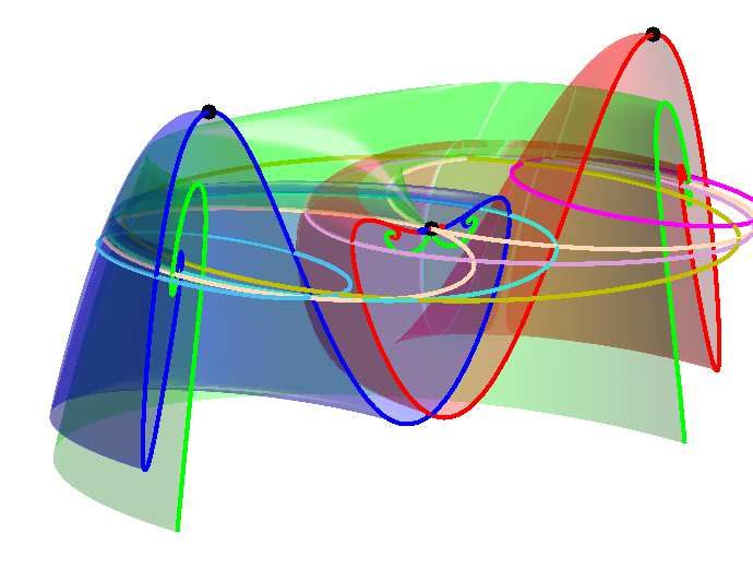
Figure 2: Family of R1 -symmetric homoclinic solutions associated with R∗ -symmetric periodic solution. Pan-
els (a1)-(a2) show two EtoP connections (blue curve) between 0 and a periodic solution Γ∗ (green curve) that
is invariant under both R1 and R2 . Panels (b1),(c1) and (b2),(c2) show temporal traces of R1 -symmetric
homoclinic solutions, associated with the connections shown in panels (a1) and (a2), respectively. Panel (d)
shows the bifurcation diagram in β2 of the EtoP connections (cyan) and R1 -symmetric homoclinic solutions,
where solutions are represented by the square of the L2 -norm of their u1 component, and each R1 -symmetric
homoclinic curve represents a family of homoclinic solutions that have the same number of humps. Notice that
the colour of a homoclinic solutions in panels (b) and (c) and their corresponding bifurcation curve in panel
(d) is the same. The black dot on the red curve corresponds to the primary homoclinic solution shown in
Fig. 1(c); the black dot and black cross on other bifurcation curves correspond to the solutions shown in panels
(1) and (2), respectively. The black dashed lines delimit the parameter interval where 0 has complex eigenvalues
with non-zero real parts; the one on the left indicates the BD bifurcation, and the one on the right the HH
bifurcation. The shaded grey region represents the region close to the purple colour parabola in Fig. 1(a). Also
shown are the bifurcation curves (light-blue) of the R1 -symmetric homoclinic solutions that have two, five, six
and seven humps. The bifurcation curves in panels (d) are for (β4 , γ, µ) = (−1, 1, 1); moreover, β2 = 0.4 in
panels (a1)-(c2).
4.1 HOMOCLINIC SOLUTIONS ASSOCIATED WITH R∗ -SYMMETRIC PE-
RIODIC SOLUTION
Heteroclinic cycles from 0 to a R∗ -symmetric periodic solution organise two main families of homoclinic solu-
tions: the R1 - and R2 -symmetric families. Furthermore, these families also organise non-symmetric homoclinic
solutions that arise when the corresponding reversibility condition is broken.
4.1.1 R1 -symmetric homoclinic solutions
Figure 2 illustrates a family of solutions associated with a R∗ -symmetric periodic solution Γ∗ along with their
bifurcation diagram. Panels (a1) and (a2) show two distinct EtoP connections (blue) from 0 to Γ∗ (green) for
(β2 , β4 , γ, µ) = (0.4, −1, 1, 1). Both these EtoP connections converge backward in time to 0 and forward in
time to Γ∗ ; however, these connections are not related by symmetry as their temporal profiles are different and
cannot be mapped to each other by any of the reversibilities or the spatial-temporal symmetry. In particular,
the EtoP connection shown in panel (a1) makes a small negative excursion in u1 and then has a transient for
positive u1 before converging to Γ∗ after t ≈ 0; in panel (a2), on the other hand, it makes two oscillation for
positive u1 before it traces Γ∗ from t ≈ 4. Since Γ∗ is R∗ -symmetric, there exist the R1 - and R2 -counterparts of
◦
the EtoP connections, which are reflections in t and rotations by 180 of panels (a), respectively. The different
combinations of these EtoP connections create different heteroclinic cycles that organise different types of
homoclinic solutions.
We first consider the heteroclinic cycle that is formed by the EtoP connection shown in panel (a1) and its
8u1 (a1) ♦ (b1) ♦ (c) ||.||2
0.8
HH
0 15
−0.8
2(a)
10
u1 (a2) ♦ (b2) ♦
0.8
0 5
(b)
(a)
−0.8
BD 1(c)
−0.75 0 0.75 t −0.75 0 0.75 t −0.5 0 0.5 β2
Figure 3: Family of R1 -symmetry broken homoclinic solutions associated with Γ∗ . Panels (a) and (b) show
temporal traces of non-symmetric homoclinic solutions associated with the connections shown in Fig. 2(a). Panel
(c) shows the bifurcation diagram in β2 of the EtoP connections (cyan) and R1 -symmetry broken homoclinic
solutions where solutions are represented by the square of the L2 -norm of their u1 component. The black
diamonds on the bifurcation curves correspond to the solutions shown in panels (a1)-(b2). Panel (c) follows
the same colour and symbols convention as Fig. 2(d) but with respect the R1 -symmetry broken homoclinic
solutions; all the homoclinic bifurcation curves from Fig. 2(d) are superimposed in light grey in panel (c). The
bifurcation curves in panels (c) are for (β4 , γ, µ) = (−1, 1, 1); moreover, β2 = 0.4 in panels (a1)-(b2).
corresponding R1 -counterpart. The temporal profiles of the u1 -component of two homoclinic solutions organised
by this cycle are shown in Fig. 2(b1) and (c1). The homoclinic solution in panel (b1) can be thought of as a
concatenation of first part of the EtoP connection in panel (a1) up to its second maximum with its R1 -symmetric
counterpart. Similarly, the homoclinic solution in panel (b2) is associated with the EtoP cycle formed by the
connection in panel (a2) and its R1 -symmetric counterpart. Two further homoclinic solutions are shown in
panels (c1) and (c2); they are derived from the EtoP connections in panels (a1) and (a2) in the same way but
for one further half-turn around Γ∗ .
This type of homoclinic solutions exist for any number of humps, including those with three and four shown in
panels (b1)-(c2). They all exhibit oscillating tails with oscillations that damp out quickly, and these homoclinic
solutions follow the respective EtoP connection in panels (a) to intersect Σ1 transversally at t = 0 where they
start following the R1 -symmetric counterpart. Hence, they are R1 -symmetric homoclinic solutions. Note that
the R2 -counterparts of the R1 -symmetric homoclinic solution also exist. However, we do not show them here
because, on the level of this figure, they correspond to reflections of u1 in the t-axis so that maxima become
minima and vice-versa.
Figure 2(d) shows the bifurcation diagram of the EtoP connections and R1 -symmetric homoclinic solutions in
the (β2 , ||u1 ||2 )-plane. Here, the dotted vertical lines bound the interval (−0.8164, 0.8164), where the equilibrium
0 is a saddle-focus; hence, this interval represents the β2 -values, between BD and HH, where homoclinic solutions
with oscillating tails exist; the shaded grey region represents the region close to the purple parabola in Fig. 1(a).
The EtoP connections in Fig. 1(a) lie on a single curve with two branches that meet at a fold at β2 ≈ 0.5753; the
EtoP connections in panels (a1) and (a2) are from the upper and the lower branch of this curve, respectively. As
the EtoP connections have an infinite L2 -norm, we represent them in panel (d) with a finite norm by truncating
the connection after ten oscillations near the periodic solution. The parameter value where they fold is the
moment where two R1 -symmetric EtoP cycles coalesce; they no longer exist beyond that value. Hence, pairs
of R1 -symmetric EtoP cycles exist for β2 ∈ (−0.8164, 0.5753) and they come together at β2 ≈ 0.5753. This
has far-reaching consequences for the organisation of the two families of R1 -symmetric homoclinic solutions
associated with Γ∗ , as is illustrated in panel (d). All R1 -symmetric homoclinic solutions also lie on curves with
two branches that meet at fold points, where two R1 -symmetric homoclinic solutions coalesce. For each curve,
the upper branch corresponds to the homoclinic solutions associated with the EtoP cycle generated by the
connection in panel (a1) and its R1 -counterpart, while the lower branch corresponds to the homoclinic solutions
associated with the EtoP cycle generated by the connection in panel (a2) and its R1 -counterpart. In Fig. 2(d),
we show the bifurcation curves of the homoclinic solutions with two to eight humps; the two curves that are
highlighted in darker colour correspond to the homoclinic solutions with three and four humps shown in panels
(b1)-(c2). Notice that all the bifurcation curves associated with the R1 -symmetric homoclinic solutions of Γ∗
fold close to β2 ≈ 0.5753. Furthermore, as the number of humps of the homoclinic solutions increases, the β2 -
values where they fold approach β2 ≈ 0.5753 from below; that is, they accumulates on the β2 -values where the
EtoP connection folds. Also shown in panel (d) is the curve of the primary homoclinic solution from Fig. 1(c),
9which exists in the entire β2 -range up to β2 ≈ 0.8164 where the eigenvalues of 0 becomes purely imaginary at
HH.
4.1.2 R1 -symmetry broken homoclinic solutions
Since there exist two distinct EtoP connections to Γ∗ , one can also consider the heteroclinic cycle that is formed
by the EtoP connection in Fig. 2(a1) and the R1 -counterpart of the EtoP connection in Fig. 2(a2), or vice-versa.
The homoclinic solutions associated with these cycles are non-symmetric and are illustrated in Fig. 3 along with
their bifurcation diagram. The homoclinic solution in panel (a1) can be thought of as a concatenation of the
first part of the EtoP connection in Fig. 2(a1) up to its second maximum with the R1 -counterpart of the EtoP
connection in Fig. 2(a2) up to its second maximum. If the concatenation is performed the other way around, the
homoclinic solution in panel (a2) is obtained; it is the R1 -counterpart of the homoclinic solution in panel (a1).
By considering one further half-turn around Γ∗ , the homoclinic solutions in panels (b1) and (b2) are derived.
In this way, non-symmetric homoclinic solutions for any number of humps can be obtained.
Note that all these non-symmetric homoclinic solutions also come in pairs, but they are each others R1 -
counterparts. Hence, in the bifurcation diagram in Fig. 3 (c) the two branches lie on top of each other and are
indistinguishable. The two branches meet at a fold point at β2 ≈ 0.5753, and they become R1 -symmetric at
this point. As before, we show the bifurcation curves of the EtoP connection and non-symmetric homoclinic
solutions from three to seven humps in panel (c). In particular, we highlight the bifurcation curves of the three-
and four-hump non-symmetric homoclinic solutions in a darker colour; moreover, all curves of the R1 -symmetric
homoclinic bifurcations from Fig. 2(d) are shown in light-grey. Note that non-symmetric and R1 -symmetric
homoclinic solutions with the same number of humps fold at the same β2 value. That is, in order to transition
between corresponding R1 -counterparts of each non-symmetric homoclinic solution, they must reach a fold point
where they become symmetric. Thus, each fold point is a symmetry-breaking of the R1 symmetry. Therefore,
we refer to this family of non-symmetric homoclinic solutions as R1 -symmetry broken homoclinic solutions of
Γ∗ .
4.1.3 R2 -symmetric and R2 -symmetry broken homoclinic solutions
There also exit cycles formed by the EtoP connections shown in Fig. 2(a) and their R2 -counterparts. In general,
we find a similar phenomenon where the corresponding cycle organises R2 -symmetric homoclinic solutions which
come in pairs. In particular, these homoclinic solutions intersect the reversibility section Σ2 transversally at
t = 0. They symmetry break at fold points and there are also associated pairs of non-symmetric homoclinic
solutions, which are R2 -symmetry broken solutions.
Figure 4 shows some representative examples of R2 -symmetric and R2 -symmetry broken homoclinic solutions
together with their bifurcation diagram. As for the R1 -symmetric homoclinic solutions, there exists a basic R2 -
symmetric homoclinic solution with one hump, which is shown in panel (a1). To illustrate the effect of the
R1 -reversibility on these R2 -symmetric homoclinic solutions, the R1 -counterpart of this solution is shown in
panel (a2). The homoclinic solutions in panels (b1)-(b2) and (c1)-(c2) have one and two further half-turns
around Γ∗ , respectively. Two non-symmetric homoclinic solutions are shown in panels (b3) and (c3); they are
associatd with the EtoP cycle formed by the EtoP connections in Fig. 2(a1) and the R2 -counterpart of the EtoP
connection in Fig. 2(a2).
Figure 4(d) shows the bifurcation diagram of the R2 -symmetric and non-symmetric homoclinic solutions
up to seven humps, and we highlight the ones with two and three humps in a darker colour. Here, all the
previously shown homoclinic bifurcation curves are shown in light grey. The basic R2 -symmetric homoclinic
solution and its R1 -counterpart shown in panels (a), exist throughout the β2 -interval where 0 has complex
conjugate eigenvalues. On the other hand, all the other R2 -symmetric homoclinic solutions lie again on curves
with two branches that meet at fold points. The new non-symmetric homoclinic solutions also come in pairs.
Since they have the same L2 -norm, the respective two branches of the bifurcation curves lie on top of each
other. All non-symmetric homoclinic solutions become R2 -symmetric at the coinciding fold points; here the R2 -
symmetry is broken, which is why we refer to them as R2 -symmetry broken homoclinic solutions. As the number
of humps per homoclinic solution increases, the parameter values where they fold accumulate on β2 ≈ 0.5753;
notice however, that this accumulation is now from larger values of β2 .
4.1.4 Connection with homoclinic snaking
It is clear from Fig. 4(d) that only the bifurcation curves of the primary R1 - and R2 -symmetric homoclinic
solutions reach the HH bifurcation; the bifurcation curves of multi-hump R1 - and R2 -symmetric homoclinic
solutions, on the other hand, have folds before reaching HH. When viewed for decreasing β2 , the two branches of
primary homoclinic solutions emerge from the HH bifurcation. It has been observed in other four-dimensional
reversible systems [39], including the Swift-Hohenberg equation [6] and the Lugiato-Lefever equation (LLE)
[30], that these primary homoclinic curves born at the HH bifurcation can undergo a phenomenon known as
10u1 (b1) • (c1) • (a1) • (a2) •
0.8
0
−0.8
−0.75 0 0.75 t −0.75 0 0.75 t −0.75 0 0.75 t −0.75 0 0.75 t
u1 (b2) × (c2) × (d) ||.||2
0.8
HH
0 15
−0.8
1(a)
10
u1 (b3) ♦ (c3) ♦
0.8
0 5
(c)
−0.8 (a)
(b)
BD
−0.75 0 0.75 t −0.75 0 0.75 t −0.5 0 0.5 β2
Figure 4: Family of R2 -symmetric and R2 -symmetry broken homoclinic solutions associated with Γ∗ . Panels (a)
show the temporal traces of the basic R2 -symmetric homoclinic solution and its corresponding R1 -symmetric
counterparts. Panels (b1),(c1) and (c2),(c3) show the temporal traces of the R2 -symmetric homoclinic solutions
associated with the EtoP connections shown in Fig. 2(a1) and Fig. 2(a2), respectively. Panels (b2) and (c2)
show non-symmetric homoclinic solutions with one and two humps, respectively. Panel (d) shows the bifurcation
diagram in β2 of the EtoP connections (cyan) and corresponding homoclinic solutions, where solutions are
represented by the square of the L2 -norm of their u1 component. Panel (d) follows the colour and symbols
convention as Fig. 2(d) but with respect the R2 -symmetric and R2 -symmetry broken homoclinic solutions; all
the homoclinic bifurcation curves from Fig. 2(d) and Fig. 3(c) are superimposed in light grey in panel (d). The
bifurcation curves in panels (d) are for (β4 , γ, µ) = (−1, 1, 1); moreover, β2 = 0.4 in panels (a1)-(c3).
homoclinic snaking: these two branches of homoclinic solutions fold back and forth repeatedly when continued
in a chosen parameter. Moreover, there exist branches of symmetry-broken homoclinic solutions that connect
the two branches of symmetric homoclinic solutions at respective fold points; these symmetry broken branches
are also referred to as “rungs” because they form a ladder-like structure with the two primary branches.
The bifurcation structure we find here for system (4) in Figs. 2–4 is quite similar in spirit, but the bifurca-
tion curves of all homoclinic solutions end for decreasing β2 at the BD bifurcation rather than featuring fold
bifurcation on the left as well. This type of bifurcation structure due to the existence of the BD bifurcation,
which we refer to as BD-truncated homoclinic snaking, was observed, for example, in [30] in a certain parameter
regime of the LLE. In contrast to the LLE, changing any of the parameters of system (4) does not qualitatively
change the bifurcation diagram in Fig. 4(d), as can be seen from the non-dimensionalisation. Thus, one cannot
find full homoclinic snaking in system (4).
The absence of homoclinic snaking means, in particular, that the branches of symmetric homoclinic solutions
with increasing numbers of humps of system (4) do not form two single connected branches. Hence, they cannot
be obtained simply by continuation of the two primary homoclinic solutions through successive fold points but
must be found one-by-one. As was explained in Sec. 3, this can be achieved efficiently with Lin’s method.
This approach has the additional advantage that it allows us to also find and continue the underlying EtoP
connections, which organise the respective branches of homoclinic solutions with different symmetry properties.
Finding branches of EtoP connections is a new aspect of our work, which shows that the β2 -values of the fold
points of homoclinic solution curves accumulate, as the number of humps increases, on the β2 -value of the fold
of the underlying EtoP connection. As we will show next, there are more such EtoP connections, including
those to periodic solutions with less symmetry.
11u1 • ×
0.8
0
−0.8
(a1) (a2)
−15 0 15 t −15 0 15 t
u1 (b1) • (c1) • (d) ||.||2
0.8
HH
0 (a)
15
−0.8
10
u1 (b2) × (c2) ×
0.8
0 (c) 5
(b)
−0.8
BD
−0.75 0 0.75 t −0.75 0 0.75 t −0.5 0 0.5 β2
Figure 5: Family of R1 -symmetric homoclinic solutions associated with R1 -symmetric periodic solution. Pan-
els (a1) and (a2) show two connections (blue curve) between 0 and a periodic solution Γ+ 1 (green curve) that
is only invariant under R1 . Panels (b1),(c1) and (b2),(c2) show temporal traces of R1 -symmetric homoclinic
solutions, associated with the connections shown in panels (a1) and (a2), respectively. Panel (d) shows the bi-
furcation diagram in β2 of the EtoP connections (cyan) and R1 -symmetric homoclinic solutions, where solutions
are represented by the square of the L2 -norm of their u1 component. All the bifurcation curves from Fig 2(d),
Fig. 3(c) and Fig. 4(d) are superimposed in light grey. Panel (d) follows the colour and symbol convention as
Fig. 2(d) but with respect to the R1 -symmetric homoclinic solutions associated with R1 -symmetric periodic
solution. The bifurcation curves in panels (d) are for (β4 , γ, µ) = (−1, 1, 1); moreover, β2 = 0.4 in panels
(a1)-(b2).
4.2 HOMOCLINIC SOLUTIONS ASSOCIATED WITH R1 -SYMMETRIC PE-
RIODIC SOLUTION
It is possible to have a (pair of) periodic solutions with only R1 -symmetry in the zero-energy level. We find
that there are EtoP connections between 0 and these periodic solutions for certain parameter values. As before,
there are associated R1 -symmetric homoclinic solutions that come in pairs and meet at fold points, where they
also symmetry break. However, we do not find R2 -symmetric and R2 -symmetry broken homoclinic solutions as-
sociated with these EtoP connections. Families of R1 -symmetric and R1 -symmetry broken homoclinic solutions
associated with an R1 -symmetric periodic solution are shown respectively in Fig. 5 and 6.
Figure 5 shows the R1 -symmetric homoclinic solutions in the same layout as Fig. 2. Panels (a1) and
(a2) show two EtoP connections, but now to an R1 -symmetric periodic solution Γ+ 1 . Note that throughout
this manuscript, the R2 -counterpart of Γ+ is denoted by Γ− , and that any results pertaining to homoclinic
solutions and EtoP connections of Γ+ also applies to Γ− . The EtoP connections in panels (a) are not related
by symmetry: the one in panel (a1) has a larger negative excursion in u1 before converging to Γ+ 1 compared to
that in panel (a2). Associated with the EtoP cycles generated by the EtoP connections in panels (a) and their
corresponding R1 -counterparts, one can find R1 -symmetric homoclinic solutions that make any number of turns
around Γ+ +
1 . Figure 5(b1) and (c1) show homoclinic solutions with one full turn around Γ1 , and panels (b2)
+
and (c2) those with one further half-turn around Γ1 . Figure 5(d) shows the corresponding bifurcation diagram,
where the two EtoP connections occur on a branch that folds at β2 ≈ 0.6756; they are again represented by a
finite norm (by truncating them after eight oscillations around the periodic solution). Also shown are curves of
the R1 -symmetric homoclinic solutions from two to five humps, where the ones in panels (b)-(c) are highlighted
in a darker colour. The curves of R1 -symmetric homoclinic solutions all have folds and, as the number of humps
increases, the β2 -values where they fold accumulate onto that of the fold of EtoP connections of Γ+1.
Figure 6 illustrates the R1 -symmetry broken homoclinic solutions, which are are associated with the EtoP
cycle generatedd by the EtoP connection in Fig. 5(a1) and the R1 -counterpart of the EtoP connection in
Fig. 5(a2), or vice versa. In Fig. 6(a) these homoclinic solutions have one turn around Γ+ 1 , while in panels
(b) they make one further half-turn. Moreover, the homoclinic solutions in panels (a2) and (b2) are the R1 -
12u1 (a1) ♦ (b1) ♦ (c) ||.||2
0.8
HH
0 5(a) 15
−0.8
10
u1 (a2) ♦ (b2) ♦
0.8
0 (a)
5
(b)
−0.8
BD
−0.75 0 0.75 t −0.75 0 0.75 t −0.5 0 0.5 β2
Figure 6: Family of R1 -symmetry broken homoclinic solutions associated with Γ+ 1 . Panels (a) and (b) show
temporal traces of non-symmetric homoclinic solutions associated with the connections shown in Fig. 5(a). Panel
(c) shows the bifurcation diagram in β2 of the EtoP connections (cyan) and R1 -symmetry broken homoclinic
solutions where solutions are represented by the square of the L2 -norm of their u1 component. Panel (c)
follows the colour and symbols convention as Fig. 2(d) but with respect to the R1 -symmetry broken homoclinic
solutions associated with R1 -symmetric periodic solution; furthermore, all the previously shown homoclinic
bifurcation curves are superimposed in light grey in panel (c). The bifurcation curves in panels (d) are for
(β4 , γ, µ) = (−1, 1, 1); moreover, β2 = 0.4 in panels (a1)-(b2).
counterparts of those in panels (a1) and (b1). As the bifurcation diagram in Fig. 6(c) shows, the R1 -symmetry
broken homoclinic connections can be found along curves that have folds at the fold points on the curves of
R1 -symmetric homoclinic connections (light grey). Here, we highlight the curves of the R1 -symmetry broken
homoclinic solutions with two and three humps in a darker colour; the respective two branches are again
indistinguishable in panel (c) because they have the same L2 -norm.
All these curves in Fig. 5(d) and Fig. 6(c) of homoclinic connections associated with Γ+ 1 extend on the left
to the BD bifurcation and, therefore, constitute a further instance of BD-truncated homoclinic snaking. In
contrast to the bifurcation curves of the homoclinic solutions associated with Γ∗ , there do not exist two primary
homoclinic bifurcation curves that arise from the HH point. Notice also that the homoclinic solutions associated
with Γ+1 exist over a larger β2 -interval; this is due to the fact that the fold of the bifurcation curve of EtoP
connection to Γ+1 has a considerably larger β2 -value than the fold of the bifurcation curve of EtoP connection
to the periodic solution Γ∗ .
5 EXISTENCE OF SOLITONS IN TWO-PARAMETER PLANEs
As we have seen in the previous sections for fixed (β4 , µ, γ) = (−1, 1, 1), infinitely many homoclinic solutions
and associated EtoP connections are created at the BD bifurcation, while only the two primary homoclinic
solutions reach the HH bifurcation. All other homoclinic solutions and the EtoP connections disappear at fold
bifurcations. We know from Sec. 2 that the BD and HH bifurcations occur along the left and right halfs of a
parabola in the (β2 , µ)-plane of Fig. 1(a) and also in the (β2 , β4 )-plane. The folds of homoclinic solutions and
EtoP connections are well defined codimension-one bifurcations that we can continue numerically as curves in
these parameter planes. However, this is not necessary because, as we show now, all fold bifurcations also occur
along half-parabolas in either of these planes; in particular, they do not depend on the parameter γ and they
always occur in the same order as a function of β2 .
To see this, we consider the ansatz U (x, τ ) = û(τ )eiqz with the non-dimensionalisation of the GNLSE (1)
for β2 > 0 and β4 < 0, which is case (c) in Table 1, to obtain the ODE
d4 û d2 û
+ 2 + qû − û3 = 0, (13)
dτ 4 dτ
On the other hand, the transformation
s s
− β4 γ − 12β2
u= u, τ0 = t
6β22 β4
13You can also read