DeepOIS: Gyroscope-Guided Deep Optical Image Stabilizer Compensation
←
→
Page content transcription
If your browser does not render page correctly, please read the page content below
DeepOIS: Gyroscope-Guided Deep Optical Image Stabilizer Compensation

                                                                                    Haipeng Li1 Shuaicheng Liu2,1 Jue Wang1
                                                                                                      1
                                                                                                  Megvii Technology
                                                                          2
                                                                              University of Electronic Science and Technology of China
arXiv:2101.11183v1 [cs.CV] 27 Jan 2021

                                                                       Abstract

                                            Mobile captured images can be aligned using their gy-
                                         roscope sensors. Optical image stabilizer (OIS) terminates
                                         this possibility by adjusting the images during the captur-
                                         ing. In this work, we propose a deep network that com-
                                         pensates the motions caused by the OIS, such that the                                                  (a)                              (b)
                                         gyroscopes can be used for image alignment on the OIS
                                         cameras1 . To achieve this, first, we record both videos and
                                         gyroscopes with an OIS camera as training data. Then, we
                                         convert gyroscope readings into motion fields. Second, we
                                         propose a Fundamental Mixtures motion model for rolling
                                         shutter cameras, where an array of rotations within a frame
                                         are extracted as the ground-truth guidance. Third, we train
                                                                                                                                                (c)                              (d)
                                         a convolutional neural network with gyroscope motions as
                                         input to compensate for the OIS motion. Once finished,                    Figure 1. (a) inputs without the alignment, (b) gyroscope align-
                                         the compensation network can be applied for other scenes,                 ment on a non-OIS camera, (c) gyroscope alignment on an OIS
                                         where the image alignment is purely based on gyroscopes                   camera, and (d) our method on an OIS camera. We replace the
                                         with no need for images contents, delivering strong robust-               red channel of one image with that of the other image, where mis-
                                         ness. Experiments show that our results are comparable                    aligned pixels are visualized as colored ghosts. The same visual-
                                         with that of non-OIS cameras, and outperform image-based                  ization is applied for the rest of the paper.
                                         alignment results with a relatively large margin.

                                                                                                                   14]. In this way, the rotational motions can be compen-
                                         1. Introduction                                                           sated. We refer to this as gyro image alignment. One draw-
                                                                                                                   back is that translations cannot be handled by the gyro. For-
                                             Image alignment is a fundamental research problem that                tunately, rotational motions are prominent compared with
                                         has been studied for decades, which has been applied in                   translational motions [34], especially when filming scenes
                                         various applications [4, 45, 12, 41, 24]. Commonly adopted                or objects that are not close to the camera [23].
                                         registration methods include homography [10], mesh-based
                                                                                                                       Compared with image-based methods, gyro-based meth-
                                         deformation [45, 22], and optical flow [8, 29]. These meth-
                                                                                                                   ods are attractive. First, it is irrelevant to image contents,
                                         ods look at the image contents for the registration, which
                                                                                                                   which largely improves the robustness. Second, gyros are
                                         often require rich textures [21, 46] and similar illumination
                                                                                                                   widely available and can be easily accessed on our daily
                                         variations [37] for good results.
                                                                                                                   mobiles. Many methods have built their applications based
                                             In contrast, gyroscopes can be used to align images,
                                                                                                                   on the gyros [15, 13, 44].
                                         where image contents are no longer required [17]. The
                                         gyroscope in a mobile phone provides the camera 3D ro-                        On the other hand, the cameras of smartphones keep
                                         tations, which can be converted into homographies given                   evolving, where optical image stabilizer (OIS) becomes
                                         camera intrinsic parameters for the image alignment [17,                  more and more popular, which promises less blurry im-
                                                                                                                   ages and smoother videos. It compensates for 2D pan and
                                           1 Code   will be available on https://github.com/lhaippp/DeepOIS.       tilt motions of the imaging device through lens mechan-

                                                                                                               1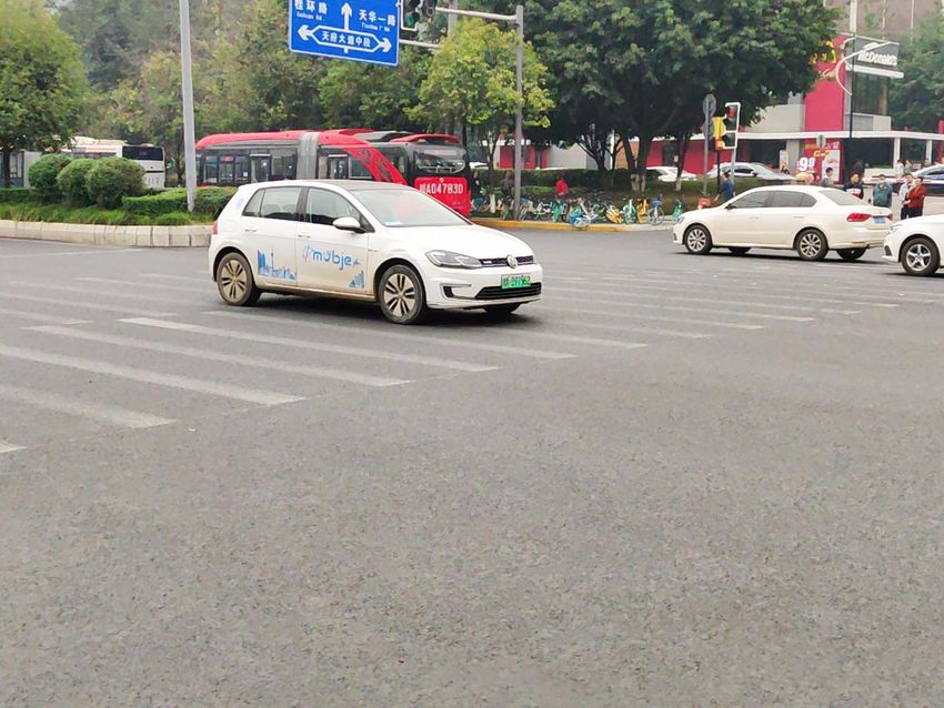
ics [5, 42]. However, OIS terminates the possibility of im-            • We propose a solution that learns the mapping func-
age registration by gyros. As the homography derived from                tion between gyro motions and real motions, where
the gyros is no longer correspond to the captured images,                a Fundamental Mixtures model is proposed under the
which have been adjusted by OIS with unknown quantities                  RS setting for the real motions.
and directions. One may try to read pans and tilts from the
camera module. However, this is not easy as it is bounded              • We propose a dataset for the evaluation. Experiments
with the camera sensor, which requires assistance from pro-              show that our method works well when compared with
fessionals of the manufacturers [19].                                    non-OIS cameras, and outperforming image-based op-
   In this work, we propose a deep learning method that                  ponents in challenging cases.
compensates the OIS motion without knowing its readings,
such that the gyro can be used for image alignment on OIS            2. Related Work
equipped cell-phones. Fig. 1 shows an alignment example.
                                                                     2.1. Image Alignments
Fig. 1 (a) shows two input images. Fig. 1 (b) is the gyro
alignment produced by a non-OIS camera. As seen, the im-                 Homography [10], mesh-based [45], and optical
ages can be well aligned with no OIS interferences. Fig. 1           flow [37] methods are the most commonly adopted motion
(c) is the gyro alignment produced by an OIS camera. Mis-            models, which align images in a global, middle, and pixel
alignments can be observed due to the OIS motion. Fig. 1             level. They are often estimated by matching image fea-
(d) represents our OIS compensated result.                           tures or optimize photometric loss [21]. Apart from clas-
   Two frames are denoted as Ia and Ib , the motion from             sical traditional features, such as SIFT [25], SURF [3], and
gyro between them as Gab . The real motion (after OIS ad-            ORB [32], deep features have been proposed for improving
justment) between two frames is G0ab . We want to find a             robustness, e.g., LIFT [43] and SOSNet [38]. Registration
mapping function that transforms Gab to G0ab :                       can also be realized by deep learning directly, such as deep
                                                                     homography estimation [20, 46]. In general, without ex-
                       G0ab = f (Gab ).                    (1)       tra sensors, these methods align images based on the image
                                                                     contents.
    We propose to train a supervised convolutional neural
network for this mapping. To achieve this, we record videos          2.2. Gyroscopes
and their gyros as training data. The input motion Gab can
                                                                         Gyroscope is important in helping estimate camera rota-
be obtained directly given the gyro readings. However, ob-
                                                                     tions during mobile capturing. The fusion of gyroscope and
taining the ground-truth labels for G0ab is non-trivial. We
                                                                     visual measurements have been widely applied in various
propose to estimate the real motion from the captured im-
                                                                     applications, including but not limited to, image alignment
ages. If we estimate a homography between them, then
                                                                     and video stabilization [17], image deblurring [26], simul-
the translations are included, which is inappropriate for
                                                                     taneous localization and mapping (SLAM) [15], gesture-
rotation-only gyros. The ground-truth should merely con-
                                                                     based user authentication on mobile devices [13], and hu-
tain rotations between Ia and Ib . Therefore, we estimate
                                                                     man gait recognition [44]. In mobiles, one important issue
a fundamental matrix and decompose it for the rotation
                                                                     is the synchronization between the timestamps of gyros and
matrix [14]. However, the cell-phone cameras are rolling
                                                                     video frames, which requires gyro calibration [16]. In this
shutter (RS) cameras, where different rows of pixels have
                                                                     work, we access the gyro data at the Hardware Abstraction
slightly distinct rotations matrices. In this work, we pro-
                                                                     Layer (HAL) of the android layout [36], to achieve accurate
pose a Fundamental Mixtures model that estimates an array
                                                                     synchronizations.
of fundamental matrices for the RS camera, such that rota-
tional motions can be extracted as the ground-truth. In this         2.3. Optical Image Stabilizer
way, we can learn the mapping function.
    For evaluations, we capture a testing dataset with various          Optical Image Stabilizer (OIS) has been around commer-
scenes, where we manually mark point correspondences for             cially since the mid-90s [33] and becomes more and more
quantitative metrics. According to our experiments, our net-         popular in our daily cell-phones. Both the image capturing
work can accurately recover the mapping, achieving gyro              and video recording can benefit from OIS, producing re-
alignments comparable to non-OIS cameras. In summary,                sults with less blur and improved stability [19]. It works by
our contributions are:                                               controlling the path of the image through the lens and onto
                                                                     the image sensor, which is achieved by measuring the cam-
   • We propose a new problem that compensates OIS mo-               era shakes using sensors such as gyroscope, and move the
     tions for gyro image alignment on cell-phones. To the           lens horizontally or vertically to counteract shakes by elec-
     best of our knowledge, the problem is not explored yet,         tromagnet motors [5, 42]. Once a mobile is equipped with
     but important to many image and video applications.             OIS, it cannot be turn-off easily [27]. On one hand, OIS is

                                                                 2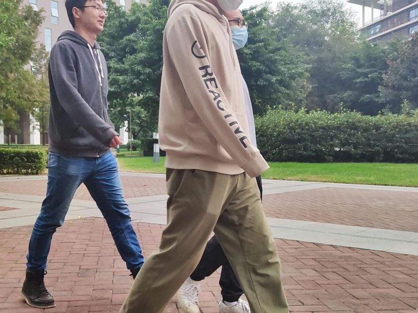
good for daily users. On the other hand, it is not friendly to
mobile developers who need gyros to align images. In this tb (i) = ta (i) + tf , (4)
work, we enable the gyro image alignment on OIS cameras. where tf = 1/F P S is the frame period. Here, the ho-
mography between the i-th row at frame Ia and Ib can be
3. Algorithm modeled as:
Our method is built upon convolutional neural networks. H = KR (tb ) R> (ta ) K−1 , (5)
It takes one gyro-based flow Gab from the source frame Ia >
to the target frame Ib as input, and produces OIS compen- where R (tb ) R (ta ) can be computed by accumulating ro-
sated flow G0ab as output. Our pipeline consists of three tation matrices from ta to tb .
modules: a gyro-based flow estimator, a Fundamental Mix- In our implementation, we divide the image into 6
tures flow estimator, and a fully convolutional network that patches which computes a homography array containing 6
compensates the OIS motion. Fig. 2 illustrates the pipeline. horizontal homographies between two consecutive frames.
First, the gyro-based flows are generated according to the We convert the homography array into a flow field [26] so
gyro readings (Fig. 2(a) and Sec. 3.1), then they are fed into that it can be fed as input to a convolutional neural network.
a network to produce OIS compensated flows G0ab as output For every pixel p in the Ia , we have:
(Fig. 2(b) and Sec. 3.3). To obtain the ground-truth rota-
p0 = H(t)p, (u, v) = p0 − p, (6)
tions, we propose a Fundamental Mixtures model, so as to
produce the Fundamental Mixtures flows Fab (Fig. 2 (d) and computing the offset for every pixel produces a gyro-based
Sec. 3.2) as the guidance to the network (Fig. 2 (c)). Dur- flow Gab .
ing the inference, the Fundamental Mixtures model is not
3.2. Fundamental Mixtures
required. The gyro readings are converted into gyro-based
flows and fed to the network for compensation. Before introducing our model of Fundamental Mixtures,
we briefly review the process of estimating the fundamen-
3.1. Gyro-Based Flow tal matrix. If the camera is global-shutter, every row of the
We compute rotations by compounding gyro readings frame is imaged simultaneously at a time. Let p1 and p2
consisting of angular velocities and timestamps. In particu- be the projections of the 3D point X in the first and sec-
lar, we read them from the HAL of android architecture for ond frame, p1 = P1 X and p2 = P2 X, where P1 and P2
synchronization. The rotation vector n = (ωx , ωy , ωz ) ∈ represent the projection matrices. The fundamental matrix
R3 is computed from gyro readings between frames Ia and satisfies the equation [14]:
Ib [17]. The rotation matrix R(t) ∈ SO(3) can be produced pT1 Fp2 = 0, (7)
according to the Rodrigues Formula [6]. T
If the camera is global shutter, the homography is mod-
T
where p1 = (x1 , y1 , 1) and p2 = (x01 , y10 , 1) .
Let f be the
eled as: 9-element vector made up of F , then Eq.(7) can be written
H(t) = KR(t)K−1 , (2) as:
x01 x1 , x01 y1 , x01 , y10 x1 , y10 y1 , y10 , x1 , y1 , 1 f = 0,
where K is the intrinsic camera matrix and R(t) denotes the (8)
camera rotation from Ia to Ib . given n correspondences, yields a set of linear equations:
In an RS camera, every row of the image is exposed at
x01 pT1 y10 pT1 pT1
a slightly different time. Therefore, Eq.(2) is not applicable
since every row of the image has slightly different rotation Af =
.. .. .. f = 0. (9)
. . .
matrices. In practice, assigning each row of pixels with a ro- x0n pTn yn0 pTn pTn
tation matrix is unnecessary. We group several consecutive
rows into a row patch and assign each patch with a rotation Using at least 8 matching points yields a homogenous linear
matrix. Fig. 3 shows an example. Let ts denotes the camera system, which can be solved under the constraint kf k2 =
readout time that is the time duration between the exposure 1 using the Singular Value Decomposition(SVD) of A =
of the first row and the last row of pixels. U DV > where the last column of V is the solution [14].
In the case of RS camera, projection matrices P1 and P2
i vary across rows instead of being frame-global. Eq.(7) does
ta (i) = tI + ts , (3)
N not hold. Therefore, we introduce Fundamental Mixtures
where ta (i) denotes the start of the exposure of the i-th assigning each row patch with a fundamental matrix.
patch in Ia as shown in Fig. 3, tI denotes the starting times- We detect FAST features [40] and track them by
tamp of the corresponding frame, N denotes the number of KLT [35] between frames. We modify the detection thresh-
patches per frame. The end of the exposure is: old for uniform feature distributions [11, 12].
3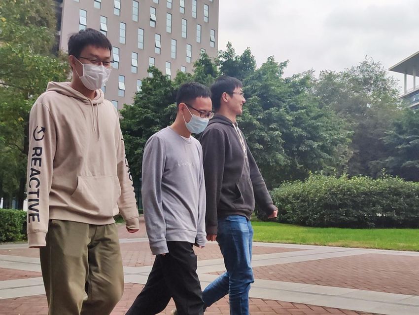
Homography Array Source Output Target Fundamental Mixtures
L1
loss
(a) Gyro-Flow estimator (b) Network structure (c) Flow loss (d) Fundamental-Flow estimator
Figure 2. The overview of our algorithm which includes (a) gyro-based flow estimator, (d) the fundamental-based flow estimator, and
(b) neural network predicting an output flow. For each pair of frames Ia and Ib , the homography array is computed using the gyroscope
readings from tIa to tIb , which is converted into the source motion Gab as the network input. On the other side, we estimate a Fundamental
Mixtures model to produce the target flow Fab as the guidance. The network is then trained to produce the output G0ab .
where fi denotes the vector formed by concatenating the
columns of Fi . Combining Eq.(11) and Eq.(12) yields a
1 × 9i linear constraint:
... ...
... ...
f1
w1 (p1 )A1p1 . . . wi (p1 )Aip1 ... = Ap1 f = 0.
(13)
fi
| {z }
Ap 1
| {z }
f
Figure 3. Illustration of rolling shutter frames. tIa and tIb are the
Aggregating all linear constraints Apj for every match point
frame starting time. ts is the camera readout time and tf denotes (pj , pj+1 ) yields a homogenous linear system Af = 0 that
the frame period (tf > ts ). ta (i) and tb (i) represent the starting can be solved under the constraint kf k2 = 1 via SVD.
time of patch i in Ia and Ib . For robustness, if the number of feature points in one
patch is inferior to 8, Eq.(13) is under constrained. There-
fore, we add a regularizer to constrain λ Aip − Ai−1
p 2
=0
To model RS effects, we divide a frame into N patches, to the homogenous system with λ = 1.
resulting in N unknown fundamental matrices Fi to be es-
timated per frame. If we estimate each fundamental ma- 3.2.1 Rotation-Only Homography
trix independently, the discontinuity is unavoidable. We
propose to smooth neighboring matrices during the esti- Given the fundamental matrix Fi and the camera intrinsic
mation as shown in Fig. 2 (d), where a point p1 not only K, we can compute the essential matrix Ei of the i-th patch:
contributes to its own patch but also influences its nearby Ei = KT Fi K. The essential matrix Ei [14] can be decom-
patches weighted by the distance. The fundamental matrix posed into camera rotations and translations, where only ro-
for point p is the mixture: tations Ri are retained. We use Ri to form a rotation-only
homography similar to Eq.(2) and convert the homography
N
X array into a flow field as Eq.(6). We call this flow field as
F (p1 ) = Fi wi (p1 ), (10)
Fundamental Mixtures Flow Fab . Note that, Ri is spatially
i=1
smooth, as Fi is smooth, so does Fab .
where wi (p1 ) is the gaussian weight with the mean equals
to the middle of each patch, and the sigma σ = 0.001 ∗ h, 3.3. Network Structure
where h represents the frame height.
The architecture of the network is shown in Fig. 2 that
To fit a Fundamental Mixtures Fi given a pair of match-
utilizes a backbone of UNet [30] consists of a series of con-
ing points (p1 , p2 ), we rewrite Eq.(7) as:
volutional and downsampling layers with skip connections.
N
X The input to the network is gyro-based flow G0ab and the
0 = pT1 Fp1 p2 = wi (p1 ) · pT1 Fi p2 , (11) ground-truth target is Fundamental Mixtures flow Fab . Our
i=1
network aims to produce an optical flow of size H × W × 2
where pT1 Fk p2 can be transformed into: which compensates the motion generated by OIS between
G0ab and Fab . Besides, the network is fully convolutional
Aip1 fi = x01 pT1 y10 pT1 pT1
fi , (12) which accepts input of arbitrary sizes.
4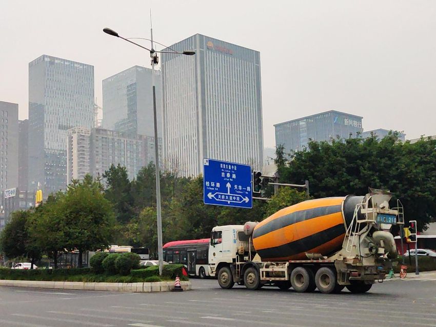
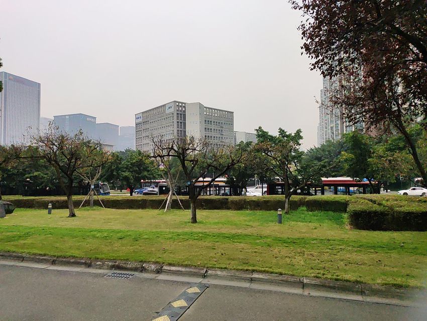
Figure 4. A glance at our evaluation dataset. Our dataset con-
tains 4 categories, regular(RE), low-texture(LT), low-light(LL)
and moving-foreground(MF). Each category contains 350 pairs,
a total of 1400 pairs, with synchronized gyroscope readings.
                                                                      Figure 5. We mark the correspondences manually in our evaluation
                                                                      set for quantitative metrics. For each pair, we mark 6 ∼ 8 point
   Our network is trained on 9k rich-texture frames with              matches.
resolution of 360x270 pixels over 1k iterations by an Adam                                   Non-OIS Camera    OIS Camera    Ours
optimizer [18] whose lr = 1.0 × 10⁻⁴ , β1 = 0.9, β2 =
                                                                         Geometry Distance        0.688           1.038      0.709
0.999. The batch size is 8, and for every 50 epochs, the
                                                                               Table 1. Comparisons with non-OIS camera.
learning rate is reduced by 20%. The entire training process
costs about 50 hours. The implementation is in PyTorch and            4.2. Comparisons with non-OIS camera
the network is trained on one NVIDIA RTX 2080 Ti.
                                                                         Our purpose is to enable gyro image alignment on OIS
                                                                      cameras. Therefore, we compare our method with non-OIS
4. Experimental Results                                               cameras. In general, our method should perform equally
4.1. Dataset                                                          well as non-OIS cameras, if the OIS motion could be com-
                                                                      pensated successfully. For comparison, ideally, we should
   Previously, there are some dedicated datasets which are            use one camera with OIS turn on and off. However, the
designed to evaluate the homography estimation [46] or the            OIS cannot be turned off easily. Therefore, we use two cell-
image deblurring with the artificial-generated gyroscope-             phones with similar camera intrinsics, one with OIS and one
frame pair [26], whether none of them combine real gy-                without, and capture the same scene twice with similar mo-
roscope readings with corresponding video frames. So we               tions. Fig. 6 shows some examples. Fig. 6 (a) shows the
propose a new dataset and benchmark GF4.                              input frames. Fig. 6 (b) shows the gyro alignment on a non-
Training Set To train our network, we record a set of videos          OIS camera. As seen, images can be well aligned. Fig. 6
with the gyroscope readings using a hand-held cellphone.              (c) shows the gyro alignment on an OIS camera. Due to the
We choose scenes with rich textures so that sufficient fea-           OIS interferences, images cannot be aligned directly using
ture points can be detected to calculate the Fundamental              the gyro. Fig. 6 (d) shows our results. With OIS compensa-
Mixtures model. The videos last 300 seconds, yielding                 tion, images can be well aligned on OIS cameras.
9,000 frames in total. Note that, the scene type is not im-              We also calculate quantitative values. Similarly, we mark
portant as long as it can provide enough features as needed           the ground-truth for evaluation. The average geometry dis-
for Fundamental Mixtures estimation.                                  tance between the warped points and the manually labeled
Evaluation Set For the evaluation, we capture scenes with             GT points are computed as the error metric (the lower the
different types, to compare with image-based registration             better). Table 1 shows the results. Our result 0.709 is com-
methods. Our dataset contains 4 categories, including reg-            parable with non-OIS camera 0.688 (slightly worse), while
ular (RE), low-texture (LT), low-light (LL), and moving-              no compensation yields 1.038, which is much higher.
foregrounds (MF) frame-gyroscope pairs. Each scene con-
                                                                      4.3. Comparisons with Image-based Methods
tains 350 pairs. So, there are 1400 pairs in the dataset. We
show some examples in Fig. 4. For quantitative evaluation,               Although it is a bit unfair to compare with image-based
we manually mark 6 ∼ 8 point correspondences per pair,                methods as we adopt additional hardware. We desire to
distributing uniformly on frames. Fig. 5 shows some exam-             show the importance and robustness of the gyro-based
ples.                                                                 alignment, to highlight the importance of enabling this ca-

                                                                  5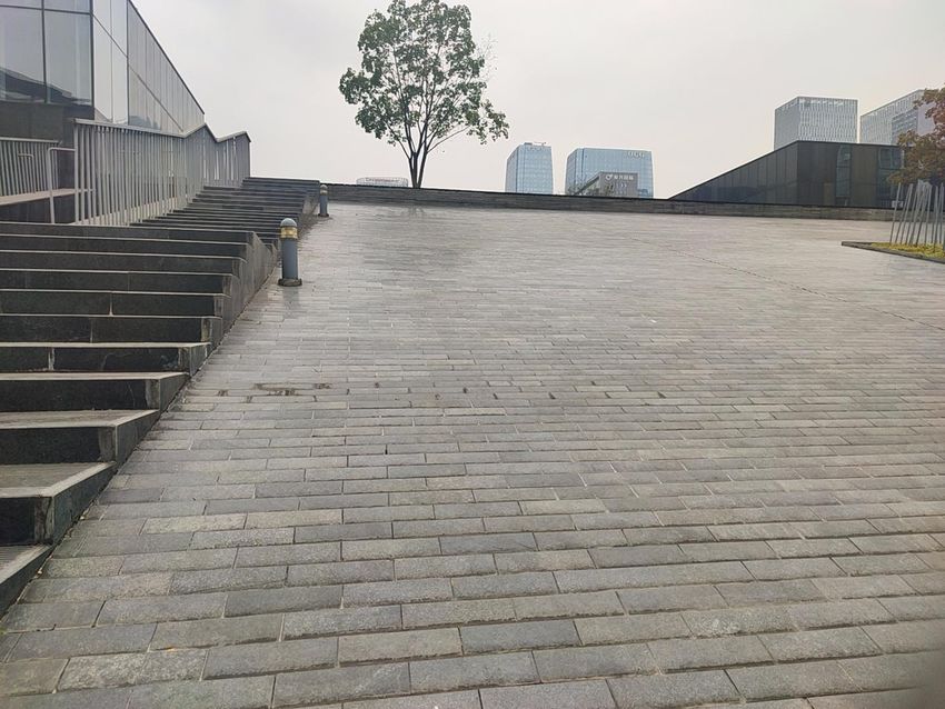
Figure 6. Comparisons with non-OIS cameras. (a) input two frames. (b) gyro alignment results on the non-OIS camera. (c) gyro alignment
results on the OIS camera. (d) our OIS compensation results. Without OIS compensation, clear misalignment can be observed in (c)
whereas our method can solve this problem and be comparable with non-OIS results in (b).

pability on OIS cameras.                                              and Fig. 7(f) is a low-texture scene. All the image-based
                                                                      methods fail as no high-quality features can be extracted,
4.3.1   Qualitative Comparisons                                       whereas our method is robust.

Firstly, we compare our method with one frequently used               4.3.2   Quantitative Comparisons
traditional feature-based algorithm, i.e. SIFT [25] and
RANSAC [9] that compute a global homography, and an-                  We also compare our method with other feature-based
other feature-based algorithm, i.e. Meshflow [22] that de-            methods quantitatively, i.e., the geometry distance. For the
forms a mesh for the non-linear motion representation.                feature descriptors, we choose SIFT [25], ORB [31], SOS-
Moreover, we compare our method with the recent deep ho-              Net [38], SURF [3]. For the outlier rejection algorithms,
mography method [46].                                                 we choose RANSAC [9] and MAGSAC [2]. The errors for
    Fig. 7 (a) shows a regular example where all the meth-            each category are shown in Table 2 followed by the overall
ods work well. Fig. 7 (b), SIFT+RANSAC fails to find a                averaged error, where I3×3 refers to a 3 × 3 identity matrix
good solution, so does deep homography, while Meshflow                as a reference. In particular, feature-based methods some-
works well. One possible reason is that a single homogra-             times crash, when the error is larger than I3×3 error, we set
phy cannot cover the large depth variations. Fig. 7 (c) illus-        the error equal to I3×3 error. Regarding the motion model,
trates a moving-foreground example that SIFT+RANSAC                   from 3) to 10) and 12) are single homography, 11) is mesh-
and Meshflow cannot work well, as few features are de-                based, and 13) is a homography array. In Table 2, we mark
tected on the background, whereas Deep Homography and                 the best performance in red and the second-best in blue.
our method can align the background successfully. A sim-                 As shown, except for comparing to feature-based meth-
ilar example is shown in Fig. 7 (d), SIFT+RANSAC and                  ods in RE scenes, our method outperforms the others for all
Deep Homography fail. Meshflow works on this example as               categories. It is reasonable because, in regular(RE) scenes,
sufficient features are detected in the background. In con-           a set of high-quality features is detected which allows to
trast, our method can still align the background without any          output a good solution. In contrast, gyroscopes can only
difficulty. Because we do not need the image contents for             compensate for rotational motions, which decreases scores
the registration. Fig. 7(e) is an example of low-light scenes,        to some extent. For the rest scenes, our method beats

                                                                  6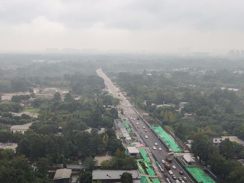
Figure 7. Comparisons with image-based methods. We compare with SIFT [25] + RANSAC [9], Meshflow [22], and the recent deep
homography [46] method. We show examples covering all scenes in our evaluation dataset. Our method can align images robustly while
image-based methods contain some misaligned regions.

the others with an average error being lower than the 2nd           rays as input. Similarly, on the other side, the Fundamental
best by 56.07%. Especially for low-light(LL) scenes, our            Mixtures are converted into rotation-only homography ar-
method computes an error which is at least lower than the           rays and then used as guidance. Fig. 8 shows the pipeline,
2nd best by 43.9%.                                                  where we test two homography representations, including
                                                                    3 × 3 homography matrix elements and H4pt representation
4.4. Ablation Studies
                                                                    from [7] that represents homography by 4 motion vectors.
4.4.1   Fully Connected Neural Network                              The network is fully connected and L2 loss is adopted for
                                                                    the regression. We adopt the same training data as described
Our network is fully convolutional, where we convert gy-            above. The result is that neither representations converge,
roscope data into homography arrays, and then into flow             where the H4pt is slightly better than directly regressing
fields as image input to the network. However, there is an-         matrix elements.
other option where we can directly input homography ar-

                                                                7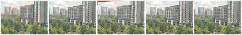
1)                                           RE                    LT                   LL                   MF                           Avg
  2) I3×3                               7.098(+2785.37%)    7.055(+350.80%)       7.035(+519.55%)      7.032(+767.08%)              7.055(+313.97%)
  3) SIFT [25]+ RANSAC [9]               0.340(+38.21%)     6.242(+298.85%)       2.312(+103.58%)      1.229(+51.54%)               2.531(+48.49%)
  4) SIFT [25] + MAGSAC [2]              0.213(−13.41%)     5.707(+264.66%)       2.818(+148.17%)       0.811(+0.00%)               2.387(+40.08%)
  5) ORB [31] + RANSAC [9]              0.653(+165.45%)     6.874(+339.23%)        1.136(+0.00%)       2.27(+179.28%)               2.732(+60.30%)
  6) ORB [31] + MAGSAC [2]              0.919(+273.58%)     6.859(+338.27%)        1.335(+17.60%)      2.464(+203.82%)              2.894(+69.83%)
  7) SOSNET [39] + RANSAC [9]            0.246(+0.00%)      5.946(+279.94%)        1.977(+74.11%)      0.907(+11.84%)               2.269(+33.14%)
  8) SOSNET [39] + MAGSAC [2]            0.309(+25.61%)     5.585(+256.87%)        1.972(+73.67%)      1.142(+40.81%)               2.252(+32.14%)
  9) SURF [3] + RANSAC [9]               0.343(+39.43%)     3.161(+101.98%)        2.213(+94.89%)      1.420(+75.09%)                1.784(+4.69%)
  10) SURF [3] + MAGSAC [2]              0.307(+24.80%)     3.634(+132.20%)        2.246(+97.78%)      1.267(+56.23%)                1.863(+9.34%)
  11) MeshFlow [22]                     0.843(+242.68%)     7.042(+349.97%)       1.729(+52.27%)       1.109(+36.74%)               2.681(+57.30%)
  12) Deep Homography [46]              1.342(+445.53%)      1.565(+0.00%)        2.253(+98.41%)       1.657(+104.32%)               1.704(+0.00%)
  13) Ours                              0.609(+147.56%)      1.01(−35.27%)        0.637(−43.90%)        0.736(−9.25%)               0.749(−56.07%)
   Table 2. Quantitative comparisons on the evaluation dataset. The best performance is marked in red and the second-best is in blue.

                                                                           Ground Truth                RE          LT          LL       MF         Avg
                                                                           Global Fundamental        0.930        1.189    0.769       0.917       0.951
                                                                           Fundamental Mixtures      0.609        1.010    0.637       0.736       0.749
                                                                          Table 3. The performance of networks trained on two different GT.

                                                                          4.4.3   Backbone
Figure 8. Regression of the homography array using the fully con-
nected network. For each pair of frames Ia and Ib , a homography
array is computed by using gyro readings, which is fed to the net-                              RE           LT           LL         MF           Avg
work. On the other side, a Fundamental Mixtures model is pro-
duced as targets to guide the training process.                              R2UNet[1]         0.713        1.006       0.652       0.791      0.791
                                                                             AttUNet[28]       0.896        1.058       0.752       0.993      0.925
                                                                             R2AttUNet[1]      0.651        1.014       0.668       0.722      0.764
   Perhaps, there exist other representations or network                     Ours             0.609    1.01    0.637 0.736 0.749
structures that may work well or even better than our current             Table 4. The performance of networks with different backbones.
proposal. Here, as the first try, we have proposed a work-
ing pipeline and want to leave the improvements as future
works.                                                                       We choose the UNet [30] as our network backbone, we
                                                                          also test several other variants [1, 28]. Except for At-
                                                                          tUNet [28], performances are similar, as shown in Table 4.
4.4.2   Global Fundamental vs. Mixtures
To verify the effectiveness of our Fundamental Mixtures                   5. Conclusion
model, we compare it with a global fundamental matrix.
Here, we choose the evaluation dataset of the regular scenes                 We have presented a DeepOIS pipeline for the compen-
to alleviate the feature problem. We estimate global funda-               sation of OIS motions for gyroscope image registration. We
mental matrix and Fundamental Mixtures, then convert to                   have captured the training data as video frames as well as
the rotation-only homographies, respectively. Finally, we                 their gyro readings by an OIS camera and then calculated
align the images with rotation-only homographies accord-                  the ground-truth motions with our proposed Fundamental
ingly. An array of homographies from Fundamental Mix-                     Mixtures model under the setting of rolling shutter cam-
tures produces an error of 0.451, which is better than an er-             eras. For the evaluation, we have manually marked point
ror of 0.580 produced by a single homography from a global                correspondences on our captured dataset for quantitative
fundamental matrix. It indicates that the Fundamental Mix-                metrics. The results show that our compensation network
tures model is functional in the case of RS cameras.                      works well when compared with non-OIS cameras and out-
    Moreover, we generate GT with the two methods and                     performs other image-based methods. In summary, a new
train our network, respectively. As shown in Table 3, the                 problem is proposed and we show that it is solvable by
network trained on Fundamental Mixtures-based GT out-                     learning the OIS motions, such that gyroscope can be used
performs the global fundamental matrix, which demon-                      for image registration on OIS cameras. We hope our work
strates the effectiveness of our Fundamental Mixtures.                    can inspire more researches in this direction.

                                                                      8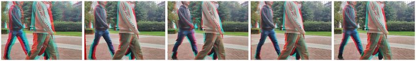
References                                                       [13] Dennis Guse and Benjamin Müller.           Gesture-
                                                                      based user authentication for mobile devicesusing ac-
 [1] Md Zahangir Alom, Mahmudul Hasan, Chris Yakop-                   celerometer and gyroscope. In Informatiktage, pages
     cic, Tarek M Taha, and Vijayan K Asari. Recur-                   243–246, 2012. 1, 2
     rent residual convolutional neural network based on
     u-net (r2u-net) for medical image segmentation. arXiv       [14] Richard Hartley and Andrew Zisserman. Multiple
     preprint arXiv:1802.06955, 2018. 8                               view geometry in computer vision. Cambridge uni-
                                                                      versity press, 2003. 1, 2, 3, 4
 [2] Daniel Barath, Jiri Matas, and Jana Noskova. Magsac:
                                                                 [15] Weibo Huang and Hong Liu. Online initializa-
     marginalizing sample consensus. In Proc. CVPR,
                                                                      tion and automatic camera-imu extrinsic calibration
     pages 10197–10205, 2019. 6, 8
                                                                      for monocular visual-inertial slam. In IEEE In-
 [3] Herbert Bay, Tinne Tuytelaars, and Luc Van Gool.                 ternational Conference on Robotics and Automation
     SURF: speeded up robust features. In Proc. ECCV,                 (ICRA), pages 5182–5189, 2018. 1, 2
     volume 3951, pages 404–417, 2006. 2, 6, 8
                                                                 [16] Chao Jia and Brian L Evans. Online calibration and
 [4] Matthew Brown and David G. Lowe. Recognising                     synchronization of cellphone camera and gyroscope.
     panoramas. In Proc. ICCV, pages 1218–1227, 2003.                 In IEEE Global Conference on Signal and Information
     1                                                                Processing, pages 731–734, 2013. 2
 [5] Chi-Wei Chiu, Paul C-P Chao, and Din-Yuan Wu. Op-           [17] Alexandre Karpenko, David Jacobs, Jongmin Baek,
     timal design of magnetically actuated optical image              and Marc Levoy. Digital video stabilization and
     stabilizer mechanism for cameras in mobile phones                rolling shutter correction using gyroscopes. CSTR,
     via genetic algorithm. IEEE Trans. on Magnetics,                 1(2011):2, 2011. 1, 2, 3
     43(6):2582–2584, 2007. 2                                    [18] Diederik P Kingma and Jimmy Ba. Adam: A
 [6] Jian S Dai.    Euler–rodrigues formula variations,               method for stochastic optimization. arXiv preprint
     quaternion conjugation and intrinsic connections.                arXiv:1412.6980, 2014. 5
     Mechanism and Machine Theory, 92:144–152, 2015.             [19] Jun-Mo Koo, Myoung-Won Kim, and Byung-Kwon
     3                                                                Kang. Optical image stabilizer for camera lens assem-
 [7] Daniel DeTone, Tomasz Malisiewicz, and Andrew Ra-                bly, Feb. 10 2009. US Patent 7,489,340. 2
     binovich. Deep image homography estimation. arXiv           [20] Hoang Le, Feng Liu, Shu Zhang, and Aseem Agar-
     preprint arXiv:1606.03798, 2016. 7                               wala. Deep homography estimation for dynamic
 [8] Alexey Dosovitskiy, Philipp Fischer, Eddy Ilg, Philip            scenes. In Proc. CVPR, pages 7652–7661, 2020. 2
     Häusser, Caner Hazirbas, Vladimir Golkov, Patrick          [21] Kaimo Lin, Nianjuan Jiang, Shuaicheng Liu, Loong-
     van der Smagt, Daniel Cremers, and Thomas Brox.                  Fah Cheong, Minh N Do, and Jiangbo Lu. Direct
     Flownet: Learning optical flow with convolutional                photometric alignment by mesh deformation. In Proc.
     networks. In Proc. ICCV, 2015. 1                                 CVPR, pages 2701–2709, 2017. 1, 2
 [9] Martin A. Fischler and Robert C. Bolles. Random             [22] Shuaicheng Liu, Ping Tan, Lu Yuan, Jian Sun, and
     sample consensus: A paradigm for model fitting with              Bing Zeng. Meshflow: Minimum latency online video
     applications to image analysis and automated cartog-             stabilization. In Proc. ECCV, volume 9910, pages
     raphy. Commun. ACM, 24(6):381–395, 1981. 6, 7,                   800–815, 2016. 1, 6, 7, 8
     8                                                           [23] Shuaicheng Liu, Binhan Xu, Chuang Deng, Shuyuan
[10] Junhong Gao, Seon Joo Kim, and Michael S                         Zhu, Bing Zeng, and Moncef Gabbouj. A hybrid
     Brown. Constructing image panoramas using dual-                  approach for near-range video stabilization. IEEE
     homography warping. In Proc. CVPR, pages 49–56,                  Trans. on Circuits and Systems for Video Technology,
     2011. 1, 2                                                       27(9):1922–1933, 2017. 1
[11] Matthias Grundmann, Vivek Kwatra, Daniel Castro,            [24] Shuaicheng Liu, Lu Yuan, Ping Tan, and Jian Sun.
     and Irfan Essa. Calibration-free rolling shutter re-             Bundled camera paths for video stabilization. ACM
     moval. In IEEE international conference on compu-                Trans. Graphics, 32(4), 2013. 1
     tational photography (ICCP), pages 1–8, 2012. 3             [25] David G. Lowe. Distinctive image features from scale-
[12] Heng Guo, Shuaicheng Liu, Tong He, Shuyuan Zhu,                  invariant keypoints. Int. J. Comput. Vis., 60(2):91–
     Bing Zeng, and Moncef Gabbouj. Joint video stitching             110, 2004. 2, 6, 7, 8
     and stabilization from moving cameras. IEEE Trans.          [26] Janne Mustaniemi, Juho Kannala, Simo Särkkä, Jiri
     on Image Processing, 25(11):5491–5503, 2016. 1, 3                Matas, and Janne Heikkila. Gyroscope-aided motion

                                                             9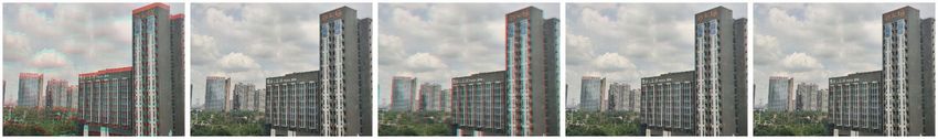
deblurring with deep networks. In 2019 IEEE Win-                [39] Yurun Tian, Xin Yu, Bin Fan, Fuchao Wu, Huub Hei-
     ter Conference on Applications of Computer Vision                    jnen, and Vassileios Balntas. Sosnet: Second order
     (WACV), pages 1914–1922. IEEE, 2019. 2, 3, 5                         similarity regularization for local descriptor learning.
[27] Steven S Nasiri, Mansur Kiadeh, Yuan Zheng, Shang-                   In Proc. CVPR, pages 11016–11025, 2019. 8
     Hung Lin, and SHI Sheena. Optical image stabiliza-              [40] Miroslav Trajković and Mark Hedley. Fast corner de-
     tion in a digital still camera or handset, May 1 2012.               tection. Image and vision computing, 16(2):75–87,
     US Patent 8,170,408. 2                                               1998. 3
[28] Ozan Oktay, Jo Schlemper, Loic Le Folgoc, Matthew               [41] Bartlomiej Wronski, Ignacio Garcia-Dorado, Man-
     Lee, Mattias Heinrich, Kazunari Misawa, Kensaku                      fred Ernst, Damien Kelly, Michael Krainin, Chia-Kai
     Mori, Steven McDonagh, Nils Y Hammerla, Bernhard                     Liang, Marc Levoy, and Peyman Milanfar. Handheld
     Kainz, et al. Attention u-net: Learning where to look                multi-frame super-resolution. ACM Trans. Graphics,
     for the pancreas. arXiv preprint arXiv:1804.03999,                   38(4):28:1–28:18, 2019. 1
     2018. 8                                                         [42] DH Yeom. Optical image stabilizer for digital pho-
[29] Jerome Revaud, Philippe Weinzaepfel, Zaid Har-                       tographing apparatus. IEEE Trans. on Consumer Elec-
     chaoui, and Cordelia Schmid. Epicflow: Edge-                         tronics, 55(3):1028–1031, 2009. 2
     preserving interpolation of correspondences for opti-           [43] Kwang Moo Yi, Eduard Trulls, Vincent Lepetit, and
     cal flow. In Proc. CVPR, pages 1164–1172, 2015. 1                    Pascal Fua. LIFT: learned invariant feature transform.
[30] Olaf Ronneberger, Philipp Fischer, and Thomas Brox.                  In Proc. ECCV, volume 9910, pages 467–483, 2016.
     U-net: Convolutional networks for biomedical image                   2
     segmentation. In International Conference on Medical            [44] Tirra Hanin Mohd Zaki, Musab Sahrim, Juliza Ja-
     image computing and computer-assisted intervention,                  maludin, Sharma Rao Balakrishnan, Lily Hanefarezan
     pages 234–241. Springer, 2015. 4, 8                                  Asbulah, and Filzah Syairah Hussin. The study of
[31] Ethan Rublee, Vincent Rabaud, Kurt Konolige, and                     drunken abnormal human gait recognition using ac-
     Gary Bradski. Orb: An efficient alternative to sift or               celerometer and gyroscope sensors in mobile applica-
     surf. In Proc. ICCV, pages 2564–2571, 2011. 6, 8                     tion. In 2020 16th IEEE International Colloquium on
                                                                          Signal Processing & Its Applications (CSPA), pages
[32] Ethan Rublee, Vincent Rabaud, Kurt Konolige, and
                                                                          151–156, 2020. 1, 2
     Gary R. Bradski. ORB: an efficient alternative to SIFT
     or SURF. In Proc. ICCV, pages 2564–2571, 2011. 2                [45] Julio Zaragoza, Tat-Jun Chin, Michael S Brown, and
                                                                          David Suter. As-projective-as-possible image stitch-
[33] Koichi Sato, Shigeki Ishizuka, Akira Nikami, and Mit-                ing with moving dlt. In Proc. CVPR, pages 2339–
     suru Sato. Control techniques for optical image stabi-               2346, 2013. 1, 2
     lizing system. IEEE Trans. on Consumer Electronics,
     39(3):461–466, 1993. 2                                          [46] Jirong Zhang, Chuan Wang, Shuaicheng Liu, Lanpeng
                                                                          Jia, Jue Wang, Ji Zhou, and Jian Sun. Content-aware
[34] Qi Shan, Wei Xiong, and Jiaya Jia. Rotational mo-                    unsupervised deep homography estimation. In Proc.
     tion deblurring of a rigid object from a single image.               ECCV, 2020. 1, 2, 5, 6, 7, 8
     In 2007 IEEE 11th International Conference on Com-
     puter Vision, pages 1–8. IEEE, 2007. 1
[35] Jianbo Shi et al. Good features to track. In 1994 Pro-
     ceedings of IEEE conference on computer vision and
     pattern recognition, pages 593–600. IEEE, 1994. 3
[36] Vividh Siddha, Kunihiro Ishiguro, and Guillermo A
     Hernandez. Hardware abstraction layer, Aug. 28 2012.
     US Patent 8,254,285. 2
[37] Deqing Sun, Xiaodong Yang, Ming-Yu Liu, and Jan
     Kautz. Pwc-net: Cnns for optical flow using pyra-
     mid, warping, and cost volume. In Proc. CVPR, pages
     8934–8943, 2018. 1, 2
[38] Yurun Tian, Xin Yu, Bin Fan, Fuchao Wu, Huub Hei-
     jnen, and Vassileios Balntas. Sosnet: Second order
     similarity regularization for local descriptor learning.
     In Proc. CVPR, pages 11016–11025, 2019. 2, 6

                                                                10
You can also read