Wainwright, T. R. O., Poole, D. J., Allen, C. B., & Appa, J. (2021). High-Fidelity Aero-Structural Simulation of Occluded Wind Turbine Blades. In ...

Wainwright, T. R. O., Poole, D. J., Allen, C. B., & Appa, J. (2021).
High-Fidelity Aero-Structural Simulation of Occluded Wind Turbine
Blades. In 2021 AIAA SciTech Forum American Institute of
Aeronautics and Astronautics Inc. (AIAA).
https://doi.org/10.2514/6.2021-0950

Peer reviewed version

Link to published version (if available):
10.2514/6.2021-0950

Link to publication record in Explore Bristol Research
PDF-document

This is the author accepted manuscript (AAM). The final published version (version of record) is available online
via AIAA at https://doi.org/10.2514/6.2021-0950. Please refer to any applicable terms of use of the publisher.

University of Bristol - Explore Bristol Research
General rights

This document is made available in accordance with publisher policies. Please cite only the
published version using the reference above. Full terms of use are available:
http://www.bristol.ac.uk/pure/user-guides/explore-bristol-research/ebr-terms/

High-Fidelity Aero-Structural Simulation of Occluded Wind
 Turbine Blades

 Thomas R. O. Wainwright∗ , Daniel J. Poole† , Christian B. Allen‡
 Department of Aerospace Engineering, University of Bristol, Bristol, UK, BS8 1TR

 Jamil Appa§ , Oliver Darbyshire¶
 Zenotech Ltd, Bristol, BS16 1EJ, UK

 A coupled, high-fidelity simulation framework on GPUs is presented, and is used to perform
 an aero-structural simulation of large wind turbines, where a turbine is fully-occluded in the
 wake of another. The GPU-enabled flow solver, zCFD, is coupled with a modal structural
 model using a multi-variate volume interpolation with radial basis functions (RBFs). Forces
 and displacements are transferred between non-coincident aerodynamic and structural models
 through the interpolation. A multi-scale RBF mesh deformation scheme is then used to
 propagate displacements through the volume mesh. A fully-meshed turbine in freestream
 flow is modelled, as well as two turbines at five diameters separation. The turbine blades
 are modified IEA 15MW blades run at the maximum IEA 15MW loading condition (95ms−1
 tip speed in flow at 25ms−1 ). A 10 million cell aerodynamic mesh is used to ensure sufficient
 capture and transport of the upstream turbine wake. Converged simulations of a fully occluded
 turbine are presented, as well as aerodynamic simulations of isolated and occluded turbines.

 I. Introduction
 Climate change, driven primarily by man-made increases in greenhouse gas concentrations, is one of the most
important factors in governmental policy making globally. This is set against the backdrop of global population increase
(which is set to reach 9.7 billion in 2050 [1]), and the continual increase in global living standards causing an exponential
increase in the desire for energy [2]. As such, a substantial drive in the development of low-emission energy production
methods has been occurring such that now, low-emission sources account for a substantial fraction of energy production
globally.
 Harvesting energy from the wind has evolved to become one of the prime alternative fuel sources. Wind turbines
harvest energy by converting kinetic energy present in the atmosphere, to rotational kinetic energy, and then to electricity
through the use of a generator. The efficiency of the first phase of this process is dictated by the aerodynamic efficiency
of the turbine blade. It is therefore critical to ensure these blades operate as close to their theoretical maximum as
possible [3].
 Advances in composite design and manufacturing technology has allowed for increasingly large rotor diameters,
maximising the energy extracted by any one turbine. This trend is seen in the increasing rotor diameters in both reference
wind turbines such as the IEA 5MW and DTU 10MW turbines [4, 5], as well as commercial turbines such as the GE
Haliade X and Seimens SG 14-222 [6, 7] However, these longer, more flexible blades are prone to strong interaction
between aerodynamic and structural dynamics during both operation and down-time. This interaction is often termed
Fluid Structure Interaction or FSI. While rotational forces can act to dampen such interactions, non-uniformities in, for
example, oncoming flow characteristics found during operation can excite interactions.
 The preferred method of deployment for wind turbines is in large-scale compact farms, minimising the geological
footprint of the farm, and reducing the required infrastructure for a fixed number of turbines. The issue arising from
farm layouts is that for any given wind direction, due to turbines yawing to the local wind direction in an attempt to
maximise a turbine’s individual power production, it is highly likely one or more turbines will be fully or partially
occluded by the wake of an upstream turbine. A simple example showing different occlusion levels of a downstream
 ∗ PhD Candidate, Email: tom.wainwright@bristol.ac.uk
 † Lecturer in Aerodynamics, AIAA Member, Email: d.j.poole@bristol.ac.uk
 ‡ Professor of Computational Aerodynamics, AIAA Senior Member, Email: c.b.allen@bristol.ac.uk
 § Co-Founder and Director at Zenotech Ltd, Email: jamil.appa@zenotech.com
 ¶ Lead CFD Engineer, Email: oliver.darbyshire@zenotech.com

 1

turbine due to the wake of an upstream turbine is shown in Figure 1. This can have severe implications both on the
power extracted by the downstream turbine due to momentum deficit in the wake, and the fatigue life of the downstream
turbine blades due to buffeting from vortices shed from the upstream turbine. With the wind energy sector tending
towards turbines using longer, more flexible blades, the ability to accurately simulate high fidelity FSI between the
blades and air in a wide range of operational conditions is of increasing interest.

 ∞
 ∞ ∞

 (a) Full occlusion (b) Partial occlusion (c) No occlusion

Fig. 1 Example of fully-occluded, partially-occluded and un-occluded downstream turbine (turbines in red,
wake boundaries in blue)

 Increasing amounts of attention have been paid to the FSI simulation and optimisation of individual turbines under
free stream conditions; see [8, 9] for example. However, the importance of determining fatigue and operational stability
of inner-farm turbines is ever increasing, particularly as more field data is obtained about the long term fatigue behaviour
of first generation wind turbines where full or partial occlusion is apparent. Oncoming flow characteristics due to
occlusion are complex, and often time-dependent due to the nature of wakes shed from upstream turbines. As such,
high-fidelity simulation is necessary to understand the impact of occlusion on efficiency, loads and fatigue, however
little work has been attempted in this area, particularly on FSI.
 The aim of this paper is to demonstrate a high fidelity FSI coupling scheme for simulation of wind turbines. In
this paper, steady state FSI modelling of turbine occlusion is considered to determine deeper insight into this aspect
of operation. Development of a large-scale multi-physics solver is presented that is based on computational fluids
dynamics (CFD) solver, zCFD ∗ and an advanced structural model developed in house at the University of Bristol,
coupled together with a generic volume interpolation-mesh motion strategy based on radial basis functions and without
the need for point reduction. Furthermore, graphics processing units (GPUs) are exploited to vastly improve run-times
and make run-times of such high-fidelity coupled simulations possible within a few hours.

 II. Background
 A review of relevant FSI simulation methods relevant to this work is presented here. For a more in-depth review
of numerical methods specifically applied to wind turbine simulations, the reader is directed to the review papers by
O’Brien et al. [10], Bai and Wang [11], and Thé and Yu [12].
 Historically the high cost associated with full CFD simulation of a wind turbine has lead to the development of lower
fidelity methods, which provide a satisfactory aerodynamic result at a much lower cost. For near wake aerodynamic
studies the actuator line and surface models developed at DTU [13–15] have been used in conjunction with LES to
provide a good flow structure. These methods provide a framework for generating the aerodynamic effects of the moving
blades to the flow, without having to obtain a full CFD solution. In most cases the aerodynamic effects of the blades are
calculated using Blade-Element-Momentum Theory (BEM).
 BEM applies two-dimensional aerodynamic coefficients to a series of finite points along the blade [3]. These
coefficients are calculated through the interpolation of lookup tables, generated using two-dimensional potential methods
such as XFoil. Through circumventing the need to perform a full CFD solution of the blade, BEM methods are
computationally much cheaper, so have found favour for studies where a high number of calculations must be performed
but aerodynamic accuracy is not the prime focus, such as structural optimisation [16–18]. Low fidelity alternatives to
BEM is have also been explored, such as the panel method developed by Boujleben et al [19], and a lifting line method,
as implemented by Sessarego et al [20].
 The major issues with BEM are that it does not account for span-wise flow effects, and it performs poorly around
stall conditions. This makes it inappropriate for application for high Tip-Speed Ratio (TSR) turbines, and turbines
 ∗ https://zcfd.zenotech.com/

 2

operating close to their stall limit during maximum energy extraction. A comparison between full CFD and BEM of
varying number of sections was performed by Lee et al [21], finding that whilst BEM methods produce reasonable
results at a low computational cost, full scale FSI was still needed to capture complex flow physics. This includes out of
plane effects, which become of increasing importance in blades with large prebend and large expected tip deflections.
This is also significant in the context of FSI of occluded turbines, as the impact of vortex buffeting is one of the key
areas of interest.
 The choice of governing fluid equations to solve in the high fidelity solution is driven by the unsteady nature of
the vortex shedding problem. Previous works have focussed on aerodynamic simulations solving both the Unsteady-
Reynolds Averaged Navier-Stokes (URANS) equations [22], as well as Large Eddy Simulation (LES) equations [23].
LES methods have been found to produce more accurate results than URANS methods, particularly in unsteady vortex
dominated flows such as those encountered in turbine wakes [12]. For FSI studies however, the difficulty encountered
with extracting accurate boundary forces from LES models, as well has the increased computational cost means URANS
remains the preferred method. A number of FSI studies have been performed examining the NREL phase VI reference
turbine [21, 24], NREL 5MW turbine [8], MEXICO reference turbine [24], and DTU 10MW reference turbine [9].
 The state-of-the-art work presented here investigates the FSI behaviour of a turbine blades using a high-fidelity,
multi-physics framework. Both isolated turbines and those operating in the fully-occluded wake of another are considered.
This is done using a fully-meshed modelling strategy with full flowfield calculations coupled to a structural solver
through a unified data interpolation and mesh motion framework.

 III. Problem Set-Up
 Throughout this paper, a modified version of the 15MW reference turbine created as part of IEA Wind TCP Task 37
is used [25]. This blade is designed to be reflective of next-generation offshore turbines, with a total turbine radius (blade
length) of 120m. The extremely large size of this blade makes it an ideal test case for FSI. Only the aerodynamic section
of the blade is modelled (i.e. the circular root is omitted) and is meshed with prebend to enable accurate modelling of
the aero-structural interaction. Finally, the trailing edge of the blade is also clam-shelled shut to create a sharp trailing
edge. The aerofoil stack of the modelled blade is shown in Figure 2.

 Fig. 2 Aerofoil stack

 For this work, isolated turbines in freestream flow are considered. In regular operation, turbines normally operate in
an atmospheric boundary layer (ABL) leading to asymmetric oncoming velocity across the disk, and with the coupling
of tower effects. However, to ensure correct development of the aero-structural solver, uniform freestream velocity
is considered initially; future work will look to introduce further effects including an ABL, tower, and hub. Due to a
uniform oncoming flow, periodicity can be exploited. In the case of the 15MW, which is three-bladed, only a single
fully-meshed blade in a 120◦ domain need to be modelled for the isolated turbine. This is shown schematically in Figure
3.
 Two cases are considered: the first is a single, unyawed, isolated turbine subject to freestream flow; the second is an
upstream turbine subject to freestream flow and a downstream turbine fully-occluded within the wake of the upstream
one, with both turbines unyawed and 5D (1200m) apart from one another. For the fully-occluded case, two 120◦ domains
are placed end-on. This models both turbines rotating in-phase at the same speed. Since, by 5D downstream, a turbine
wake has fully-formed into a gross flow with a wake deficit, this is a fine assumption. To represent two turbines with

 3

 ( )

 ∞
 Isolated Periodicity
 turbine
 − − − 
 − − 

 Fig. 3 Modelling strategy employed

out-of-phase and/or with different rotational speeds, a full 360◦ domain would be required.
 The simulated flow condition is the worse-case-scenario from an operational standpoint. The oncoming air is a
uniform freestream at sea-level conditions with a velocity of 25 −1 , which is the cut-out speed of the IEA 15MW. The
turbine is run at a tip-speed of 95 −1 , which is the maximum tip-speed of the IEA 15MW.

 IV. Aero-Structural Solver
 In this section, the CFD solver, structural solver and coupling approach are detailed. Details of GPU implementation
are also given.

A. Flow Solver
 The CFD solver zCFD† by Zenotech is used, which uses an unstructured mesh format. For viscous simulations, the
RANS equations are solved using a cell-centred finite volume scheme, with 3rd order spacial accuracy. Turbulence is
simulated through the use of Menter’s SST turbulence model [26], with the addition of wall functions in the presence of
large initial cell heights. Time marching is achieved through a five-stage Runge-Kutta scheme, with local timestepping
and geometric multigrid to accelerate convergence. For inviscid simulations, the Euler equations are solved using the
same finite volume and temporal integration schemes.
 This solver takes advantage of parallelisation through METIS partitioning, and GPU acceleration through CUDA.
Parallelisation across multiple cores is achieved through the use of MPI and OpenMP. The code is run on multiple P100
GPU cores split across multiple nodes on the University of Bristol’s Blue Crystal Phase 4 cluster‡ .
 This high level of parallelisation allows for easy simulation of large scale problems. An example of the application
of this solver to wind energy applications is the RANS simulation of Horns Rev wind farm using actuator disks, shown
in Figure 4. This simulation uses a 20 million cell unstructured mesh, with 80 turbine zones using uniform actuator
disks reflective of Vestas V-80 turbines. The free stream velocity is set to 8 −1 at hub height, with a wind direction of
280◦ . This example is intended to serve as a demonstration of the solver’s capabilities and applicability to wind energy
applications.

 Fig. 4 Simulated hub-height velocity magnitude of Horns Rev
 † https://zenotech.com/zcfd-zenotech-computational-fluid-dynamics/
 ‡ https://www.bristol.ac.uk/acrc/

 4

B. Meshing
 The meshes used in this study are structured multiblock periodic meshes, generated using the software developed by
Allen [27, 28]. The mesh uses a C-H topology wrapped around the blade, which can be seen in Figure 5. Improvements
in mesh generation are achieved through orthogonal smoothing and transfinite interpolation [29]. Whilst studies have
been conducted using unstructured meshes, such as that of Wang et al.[30], a structured mesh is preferred in this study
due to the improved accuracy at the blade surface, ensuring accurate loadings are obtained to translate to the structural
model.

 Fig. 5 Multiblock mesh topology at k=50 plane (0.49R)

C. Solver and Mesh Validation
 The rotary mesh function of the solver and the mesh generation has been validated using the Caradonna-Tung
rotor [31]. The Caradonna-Tung rotor is a 2-bladed rotor with each blade having an aspect ratio of 6, and a constant
NACA0012 profile. Two test cases were simulated that had typical tip speeds of a wind turbine. Both have an 8◦
collective angle with tip Mach numbers of 0.225 and 0.439. A 5.5 million cell 180◦ periodic volume mesh is used,
shown in Figure 6, with the surface mesh shown in Figure 7.

 5

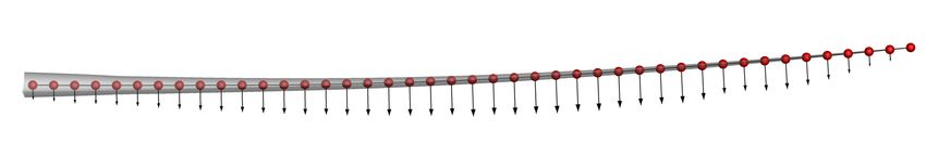
Fig. 7 Caradonna-Tung surface mesh

 Fig. 6 Caradonna-Tung block structure

 Viscous simulations using Menter’s SST turbulence model [26] with wall functions is used, with five-stage
Runge-Kutta time-marching, and multigrid acceleration. The solver is run on the University of Bristol’s parallel HPC
cluster- Blue Crystal Phase 4. A single node is exclusively used, utilising 2 NVIDIA P100 GPUs.
 The resulting flowfield of the higher speed case is shown in Figure 8, with an iso-surface of eddy viscosity and blade
surface pressures. Comparison of the experimental surface pressure distributions of the two cases is shown in shown in
Figure 9, showing excellent agreement across the blade span for both test cases.

 Fig. 8 Iso-surface for Eddy Viscosity for = 0.439 Caradonna-Tung test case

D. Structural Solver
 The structural solver is from the University of Bristol’s Aeroelastic Turbine Optimisation Methods (ATOM) [32, 33]
tool. ATOM is a full wind turbine optimisation framework that uses a blade element momentum (BEM) model to
determine aerodynamic forces and a variety of structural solvers, including both linear and non-linear finite element
with static and dynamic equations. For this work, the finite element modal solver in ATOM is employed. The structural
model and modes of the IEA 15MW turbine are predefined and used directly in ATOM. A 43-node beam-stick model
and the first six structural modes are used here. Figure 10 shows the structural model inside the blade surface, which

 6

-1.5 -1.5
 Exp. r=0.5 Exp. r=0.5
 Exp. r=0.68 Exp. r=0.68
 Exp. r=0.89 Exp. r=0.89
 -1 zCFD r=0.5 -1 zCFD r=0.5
 zCFD r=0.68 zCFD r=0.68
 zCFD r=0.89 zCFD r=0.89

 -0.5 -0.5
 Cp

 Cp
 0 0

 0.5 0.5

 1 1
 0 0.2 0.4 0.6 0.8 1 0 0.2 0.4 0.6 0.8 1
 x/c x/c

 (a) = 0.225 (b) = 0.439

Fig. 9 Comparison of simulated surface pressure coefficients with experiment for Caradonna-Tung rotor at
two different rotation speeds

shows the undeflected blade and the blade after a BEM-coupled structural solution with ATOM).

 Fig. 10 Structural nodes of IEA 15MW model (undeformed and deformed after an ATOM (BEM) solve)

E. CFD-CSD Coupling Scheme
 In order to solve FSI problems, two separate solutions need to be obtained- the aerodynamic solution, and the
structural solution. These can either be solved using a single combined code- known as the Monolithic method, or
through two separate specialised solvers, which are then coupled via methods such as Spring Analogy, Constant Volume
Transforms (CVT), or Radial Basis Functions (RBF). In recent years the separated approach has become more popular,
facilitated by advances in schemes used to couple the two results. Due to different requirements for CFD and CSD
solvers the meshes used will be different (and likely, non-coincident), and will therefore require information to be
transferred between surface nodes of each mesh. The structural mesh requires surface forces to be transferred from
the aerodynamic surface to the structural surface, and the aerodynamic mesh requires the transfer of structural mesh
displacements to the aerodynamic surface.
 The manner in which this coupling is achieved can be broken down into three categories depending on how
information is transferred at each time step. A schematic demonstrating this information transfer is shown in Figure 11,
where represents a force data transfer, and Δ represents a displacement transfer. Loose coupling [8, 21] performs a
one way information transfer at the same time step. Staggered coupling [9] iterates the two solutions at slightly different
time steps. Strong coupling [24, 34] performs multiple information transfers per time step, ensuring the result is fully
converged at each point in time. Strong coupling comes at the highest computational cost, but provides the most accurate

 7

results, particularly for unsteady effects such as flutter and buffeting.

 t t+1 t+2 t+3 t t+1 t+2 t+3 t t+1 t+2 t+3
 Fluid Fluid Fluid

 Δx

 Δx

 Δx
 
 Structure Structure Structure
 t t+1 t+2 t+3 t- t+1- t+2- t+3- t t+1 t+2 t+3
 (a) Weak (b) Staggered (c) Strong

 Fig. 11 Schematic of different coupling schemes

 Whilst a 2016 study by Heinz et al found that loose coupling is generally sufficient for generating accurate FSI results
for high fidelity turbine simulations [35], this was proven on single turbines under steady inflow conditions. Due to the
highly unsteady nature of this problem and the complex flow physics to be encountered however, strong coupling is used
throughout this work. Initially just a single steady state loop is solved until the solution is fully converged. Solving to
this state in pseudo time allows for unsteady solutions to be obtained through marching the same scheme in real time.

1. Radial Basis Function Interpolation
 Coupling between the aerodynamic surface and structural model is achieved through the use of a multivariate volume
interpolation using Radial Basis Functions (RBFs), as outlined by Rendall and Allen [36]. RBFs have the benefit of
being both mesh and connectivity independent; provided a list of surface nodes for both the aerodynamic and structural
surfaces, the information can easily be transferred. The theory of RBFs is presented comprehensively by Buhmann [37]
and Wendland [38], while the formulation pertaining to the data interpolation is presented here. A real function, (x),
can be approximated by fitting an interpolation function, (x), through known data sites, where the -th data site in
three-dimensional space is x = [ , , ] . The interpolation at a point in space, x = [ , , ] , is then given by:
 
 Õ
 (x) ≈ (x) = (||x − x ||) + (x) (1)
 =1

where is an RBF coefficient, is the RBF function adopted (such as a Wendland functions [38]), and (x) is an
optional polynomial. The polynomial can be used in mesh motion to recover translation and rotation, though is often
omitted to avoid motion of the farfield. However, at least a linear polynomial must be included for the data transfer
between aerodynamic and structural nodes to ensure conservation of total force and moment. A linear polynomial in the
 -direction (equivalent and expressions are also formed) is of the form:

 (x) = 0 + + + (2)
 The RBF coefficients can be found through requiring exact recovery of the original function at the known data
sites. In the presence of the polynomial, the system is completed by the ‘side condition’:
 
 Õ
 (x) = 0 ∀ (x) | deg (x) ≤ deg (x) (3)
 =1

 The compact generic matrix formulation of the generic system is now presented. Setting-up an interpolation between
a set of control sites, {x 1 , . . . , x }, requiring exact recovery at the sites and using the side condition, the system is
written as:

 X = (4)
 
 Y = (5)
 Z = (6)

where:

 8

 0  0 0 0 0 1 ... 1   
      0
  0  0 0 0 0 1 ...    
     
      
  0  0 0 0 0 1 ...   
     
 X = 
  0 
  , = 0
  0 0 0 1 ...  , =  
  
 (7)
      
  1  1 1 1 1 1 , 1 ... 1 ,   1 
      
  ..   .. .. .. .. .. .. ..   .. 
  .  . . . . . . .   . 
     
   1 , 1 ... ,   
     
(with analogous definitions for and ) and:

 , = (||x − x ||) (8)
Hence, is the matrix of RBFs evaluated between all of the control sites and is size + 4 × + 4. The system is
solved to find the RBF coefficients:

 = −1
 X (9)
 
 = −1
 Y (10)
 
 = −1
 Z (11)

 Once the interpolation is constructed, it can be evaluated at number of evaluation sites, {x 1 , . . . , x } from
equation 1, which in compact form is given by (with analogous definitions for and variables):

 X = = −1
 X = H X (12)
where the coupling matrix is the matrix of RBFs (plus the polynomial terms if applicable) between the variable and
evaluation sites:
 1 1 1 1 1 , 1 ... 1 , 
 
 . .. .. .. .. .. .. 
 =  .. . . . . . . , (13)
  
 1 , 1 ... , 
 
and H is termed the interpolation matrix. However, it should be noted that for memory efficiency reasons in the
mesh motion, this matrix is never fully constructed. Rather, the interpolation is determined at each evaluation point
individually, as explained in the ‘operation-intensive’ approach in Kedward et al. [39].
 There are many forms for the RBF itself (e.g. Gaussian, thin plate spine, Euclid’s hat), but the functions of Wendland
[38] provide a definable smoothness level and a definable radius of influence, as well as showing numerical properties
suitable for these types of problems [36]. The 2 function is used throughout, which varies by a distance from a point
of origin, given by:

 ( ) = (1 − )+4 (4 + 1) (14)
where (1 − )+ is the ‘cut-off ’ function which is (1 − ) if ≤ 1, or 0 otherwise. The Euclidean distance argument of the
RBF is therefore a scaled distance, which is scaled by the support radius, . The support radius therefore controls the
distance of influence of the interpolation and ensures compact support. Careful choice of the support radius is required
to balance a smooth interpolation with a numerically stable system.

2. Data Interpolation
 A two-way complementary data interpolation is formed to interpolate displacements from the structure to the
aerodynamic surface, and the subsequent forces from the surface back to the structure. Structural nodal displacements,
[ x , y , z ] are interpolated to aerodynamic surface nodal displacements by:

 9

 x = H x (15)
 y = H y (16)
 z = H z (17)
where the interpolation matrix H is formed using the structural nodes as the control sites and the aerodynamic surface
nodes as the evaluation sites.
 The aerodynamic surface forces, [f , g , h ] , are interpolated to the structural nodes by:

 f = H f (18)
 g = H g (19)
 h = H h (20)
where the interpolation matrix H is formed using the aerodynamic surface nodes as the control sites and the structural
nodes as the evaluation sites. For both interpolations, a linear polynomial is used to ensure conservation.

3. Mesh Motion
 Once structural displacements are interpolated to the aerodynamic surface, the volume mesh must subsequently
deform. For mesh deformation to occur, the farfield must remain fixed. For this, a compactly supported function is
required with a support radius that does not extend to the farfield (if a non-compact function is used then farfield motion
can be fixed by using the farfield nodes as control sites with a zero deformation specified), as well as omitting the
polynomial. Deformation of the aerodynamic mesh points, [ x , y , z ] is given by:

 x = H x (21)
 y = H y (22)
 z = H z (23)
where the interpolation matrix H uses the aerodynamic surface points as control sites and the volume mesh as
interpolation points. In the case of volume mesh displacement, the use of of H is limited by memory due to its
 × in size where is the number of volume mesh nodes, and are the number of aerodynamic surface nodes.
For the smaller 5 million cell turbine mesh this would correlate to an approximate 5, 000, 000 × 20, 000 array, occupying
400GB of memory if floats are used. Instead, H is constructed row by row at each interpolation phase.
 Constructing the interpolation matrix requires solving a × (where is the number of aerodynamic surface
points), which for large meshes becomes computationally difficult. To reduce the size of the system, work by Rendall
and Allen [40] used a greedy point selection to reduce the number of surface points used. However, later work by
Kedward et al. [39] superseded this by introducing the multiscale method. The multiscale RBF method is used here for
mesh motion.
 This unified coupling scheme allows the translation of forces from the aerodynamic surface onto the structural nodes,
and then the subsequent structural deformations to the aerodynamic surface, and ultimately to the aerodynamic volume
mesh. This procedure has been demonstrated to be effective in producing accurate high-fidelity aero-structural results
[41].

F. Coupled Solver
 The flow solver fits within an overall zCFD environment. The solver itself is partitioned into a front-end and
back-end, with Python scripting handling the front-end. The ability to compute on both and GPUs is fully exploited
here. Here, data interpolation and the structural solver are coupled into the zCFD environment front-end. Once data
initialisation has occurred on the CPU, flow updates are performed on the GPU for rapid computation times. Data can
be passed to and from the devices. For this work, aerodynamic surface forces are transferred to the CPU where the
interpolations, structural solution and mesh motion are computed. The deformed mesh is then transferred back to the
GPU for the ongoing flow updates. Figure 12 shows a schematic of the overall process, including key data flow between
the devices. It should also be noted that during set-up, if a GPU is not available, the code can be run entirely on the CPU.

 10

CPU
 Initialisation

 GPU
 Force interpolation
 f ,g ,h 
 f ,g ,h 

 ATOM

 Flow update Δx ,Δy ,Δz 
 Displacement
 interpolation
 Δx ,Δy ,Δz 
 x ,y ,z 
 Mesh motion

 Post-process

 Fig. 12 Code structure and device workflow

 V. Aerodynamic Simulations
 Before progressing to fully-coupled simulations, aerodynamic simulations are presented of both the isolated turbine,
and the two-turbine fully-occluded case. As shown in Figure 3, periodicity is employed for the cases meaning that the
fully-occluded case is a simulation of two turbines rotating at the same speed in-phase with each other. The domain
(and multi-block) structure is shown in Figure 13. Since the longitudinal separation between the turbines is 5-D, the
wake of the upstream turbine is fully-developed into a gross wake deficit region, so any out-of-phase or minor difference
in rotation speed would have a negligible effect.

 Fig. 13 Structure of occluded case

 For the single turbine, a 5 million cell mesh is used, with refinement in the near wake. For the two turbine case, a 10
million cell mesh is used. The two turbines are spaced 5-D apart in the streamwise direction (no lateral offset) with
a balance of refinement in the near wake of both turbines with good capture of the upstream turbine’s far wake (i.e.
between the turbines). The single turbine case was run to convergence on two P100 GPUs and took 4.2 hours, while the
two turbine case was run on four GPUs for 13.5 hours. This solution was conservatively run to a much higher number of

 11

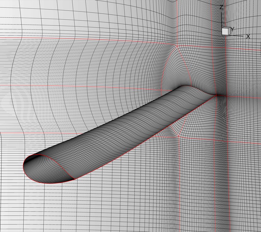
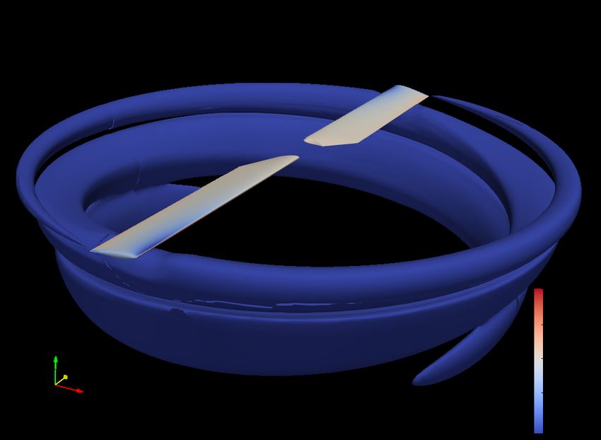
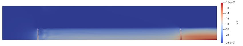
iterations (40,000) to guarantee full wake propagation from the upstream to downstream turbine. Upon inspection of the
convergence history and development of the flow solution it was found a converged solution was obtained in fewer than
10,000 cycles.
 The near wake structure of the single turbine is shown in Figure 14, showing successful capture of the wake. The
iso-surface, which is vorticity, clearly dissipates quickly and forms a gross wake deficit structure that is typical of wind
turbines.

 Fig. 14 Near-wake structure of isolated turbine

 The surface pressure coefficient distributions of the two turbine case are shown in Figure 15, which shows both the
upstream and downstream turbine. Three radial stations are shown (25%, 50% and 75%). It is first worth noting the
extremely high suction peaks around the blades. However, these are inviscid simulations at low speed, so reductions in
pressure peaks would be expected for viscous flows, or high speed flows causing shocks. These pressure peaks are a
correct representation for these aerofoil sections in inviscid flow. Furthermore, it is clear the occluded (downstream)
turbine has a lower overall loading across the blade. Considering Figure 16 also (which gives streamwise velocity), the
upstream wake is occluding the downstream turbine, as expected.

 r/R=0.25 r/R=0.25
 -8 r/R=0.5 -8 r/R=0.50
 r/R=0.75 r/R=0.75

 -6 -6
 Cp

 Cp

 -4 -4

 -2 -2

 0 0

 0 0.2 0.4 0.6 0.8 1 0 0.2 0.4 0.6 0.8 1
 x/c x/c

 (a) Upstream turbine (b) Downstream turbine

 Fig. 15 Surface pressure coefficients of upstream and downstream turbines

 12

Fig. 16 Occluded case streamwise velocity contours

 VI. Aero-Structural Simulations
 As the aerodynamic simulations show the expected behaviour, aero-structural simulations were subsequently run for
the occluded case. To do this, the converged aerodynamic solution was used to initiate the flow. Subsequent coupling
cycles were performed which involved a structural solution for each turbine followed by further flow solver iterations to
obtain a converged solution per coupled cycle until full convergence was achieved. Interpolated forces on the structural
model are shown in Figure 17.

 (a) − plane (b) − plane

 Fig. 17 Loaded structural model

 The final converged solution of the downstream turbine blade is shown in Figure 18. The final deflection at the tip of
the aeroelastic blade is 2.23m. The full solution took 15.5 hours to run on four P100 GPUs, which was made up of 13.5
hours for the initial flow solution and 2 hours for the coupling cycles.

 Fig. 18 Occluded turbine blade static (blue) and aeroelastic (red) solution

 VII. Conclusions and Future work
 A high-fidelity aerodynamic-structural coupled simulation framework has been presented and applied to flexible
wind turbines. The GPU-enabled flow solver framework, zCFD, has been used to couple the solver with a structural
model via a radial basis function interpolation. The flow solver has the ability to run on CPUs and GPUs making the
framework powerful and flexible, with large efficiency gains possible.
 The primary case considered is where a wind turbine is fully-occluded by the wake of an upstream turbine. A 10
million cell aerodynamic mesh is used to ensure good capture of the wake occlusion, and its effect on the downstream
turbine. The turbine blade used was a modified version of the IEA 15MW turbine, and was run at the IE 15MW
maximum tip speed and maximum flow speed. The solution was run on four NVIDIA P100 GPUs, with a full Euler
flow solution on the undeformed mesh performed initially followed by coupling iterations. While only inviscid flow was
considered initially to test the framework, expected results were obtained with the 120m radius turbine having a 2.2m tip
deflection.

 13

Future work will move towards performing viscous simulations and develop the framework further to be able to
perform dynamic simulations to assess fatigue. In the long-term this work will look to include the atmospheric boundary
layer and demonstrate a variety of test cases to show the flexibility of the developed framework.

 VIII. Acknowledgements
 This work was undertaken with funding from the UK Engineering and Physical Sciences Research Council Doctoral
Training Programme EP/R513179/1. The HPC resources of Bristol ACRC§ were used for numerical simulations, notably
Blue Crystal Phase 4 for highly parallel GPU simulations. The authors would like to thank David Standingford, James
Sharpe, and the other staff at Zenotech for their continued support and collaboration throughout the project. Thanks also
to Sam Scott and Terence Macquart for providing and supporting ATOM.

 References
 [1] United Nations, Department of Economic and Social Affairs, Population Division, “World Population Prospects 2019: Ten Key
 Findings,” , 2019.

 [2] U.S. Energy Information Administration, “International Energy Outlook 2019,” , 2019.

 [3] Burton, T., Jenkins, N., Sharpe, D., and Bossanyi, E., Wind Energy Handbook, 2nd ed., Wiley, John Wiley & Sons LTD, The
 Atrium, Southern Gate, Chichester, West Sussex, PO19 8SQ, United Kingdom, 2011.

 [4] Jonkman, J., Butterfield, S., Musial, W., and Scott, G., “Definition of a 5-MW Reference Wind Turbine for Offshore System
 Development,” Tech. rep., National Renewable Energy Laboratory, 2009.

 [5] Bak, C., Zahle, F., Bische, R., Kim, T., Yde, A., Henriksen, L. C., Natarajan, A., and Hansen, M., “Description of the DTU
 10MW Reference Wind Turbine,” Tech. rep., DTU Wind Energy, 2013.

 [6] “GE Haliade X Specifications,” URL https://www.ge.com/renewableenergy/wind-energy/offshore-wind/
 haliade-x-offshore-turbine, accessed: 8-12-2020.

 [7] “Siemens 12MW turbine specifications,” URL https://www.siemensgamesa.com/en-int/products-and-services/
 offshore/wind-turbine-sg-14-222-dd, accessed: 8-12-2020.

 [8] Dose, B., Rahimi, H., Herráez, I., Stoevesandt, B., and Peinke, J., “Fluid-structure coupled computations of the NREL 5MW
 wind turbine by means of CFD,” Renewable Energy, Vol. 129, 2018, pp. 591–605.

 [9] Sayed, M., Lutz, T., Krämer, E., Shayegan, S., and Wüchner, R., “Aeroelastic analysis of 10MW wind turbine using CFD-CSD
 explicit FSI-coupling approach,” Journal of Fluids and Structures, Vol. 87, 2019, pp. 354–377.

[10] O’Brien, J., Young, T., O’Mahoney, D., and Griffin, P., “Horizontal axis wind turbine research: A review of commecial CFD,
 FE codes and experimental practices,” Progress in Aerospace Sciences, Vol. 92, 2017, pp. 1–24.

[11] Bai, C.-J., and Wang, W.-C., “Review of computational and experimental approaches to analysis of aerodynamic performance
 in horizontal-axis wind turbines,” Renewable and Sustainable Energy Reviews, Vol. 63, 2016, pp. 506–519.

[12] Thé, J., and Yu, H., “A critical review on the simulations of wind turbine aerodynamics focusing on hybrid RANS-LES methods,”
 Energy, Vol. 138, 2017, pp. 257–289.

[13] Troldborg, N., “Actuator Line Modeling of Wind Turbine Wakes,” Ph.D. thesis, Department of Mechanical Engineering,
 Technical University of Denmark, 2008.

[14] Sørensen, J., and Shen, W. Z., “Numerical Modeling of Wind Turbine Wakes,” Journal of Fluids Engineering, Vol. 124, 2002,
 pp. 393–399.

[15] Shen, W. Z., Sørensen, J. N., and Zhang, J., “Actuator surface model for wind turbine flow computations,” Proceedings of
 European Wind Energy Conference, 2007.

[16] Fischer, G. R., Kipouros, T., and Savill, A. M., “Multi-objective optimisation of horizontal axis wind turbine structure and
 energy production using aerofoil and blade properties as design variables,” Renewable Energy, Vol. 62, 2014, pp. 506–515.
 § https://www.bristol.ac.uk/acrc/

 14

[17] Monte, A. D., Betta, S. D., Castelli, M. R., and Benini, E., “Proposal for a coupled aerodynamic-structural wind turbine blade
 optimization,” Composite Structures, Vol. 159, 2017, pp. 144–156.

[18] Yang, H., Chen, J., Pang, X., and Chen, G., “A new aero-structural optimization method for wind turbine blades used in low
 wind speed areas,” Composite Structures, Vol. 207, 2019, pp. 446–459.

[19] Boujleben, A., Ibrahimbegovic, A., and Lefrançois, E., “An efficient computational model for fluid-structure interaction in
 application to a large overall motion of wind turbine with flexible blades,” Applied Mathematical Modelling, Vol. 77, 2020, pp.
 392–407.

[20] Sessarego, M., Feng, J., Ramos-García, N., and Horcas, S. G., “Design optimization of a curved wind turbine blade using
 neural networks and an aero-elastic vortex method under turbulent inflow,” Renewable Energy, Vol. 146, 2020, pp. 1524–1535.

[21] Lee, K., Huque, Z., Kommalapati, R., and Han, S.-E., “Fluid-structure interation analysis of NREL phase VI wind turbine:
 Aerodynamic force evaluation and strucutral analysis using FSI analysis,” Renewable Energy, Vol. 113, 2017, pp. 512–531.

[22] Lienard, C., Boisard, R., and Daudin, C., “Aerodynamic behavior of a floating offshore wind turbine,” AIAA SciTech Forum,
 Washington, DC, 2019. AIAA Paper 2019-1575.

[23] Sedaghatizadeh, N., Arjomandi, M., Kelso, R., and Cazzolato, B., “Modelling of wind turbine wake using large eddy simulation,”
 Renewable Energy, Vol. 115, 2018, pp. 1166–1176.

[24] Carrion, M., Steijl, R., Woodgate, M., Barakos, G., and Munduate, X., “Aeroelastic analysis of wind turbines using a tightly
 coupled CFD–CSD method,” Journal of Fluids and Structures, Vol. 50, 2014, pp. 392–415.

[25] Gaertner, E., Rinker, J., Sethuraman, L., Zahle, F., Anderson, B., Barter, G., Abbas, N., Meng, F., Bortolotti, P., Skrzypinski, W.,
 Scott, G., Feil, R., Bredmose, H., Dykes, K., Shields, M., and Viselli, C. A. A., “Definition of the IEA 15-Megawatt Offshore
 Reference WInd Turbine,” Tech. rep., National Renewable Energy Laboratory, 2020.

[26] Menter, F., “Two-Equation Eddy-Viscosity Turbulence Models for Engineering Applications,” AIAA Journal, Vol. 32, 1994, pp.
 1598–1605.

[27] Allen, C., “Multigrid convergence of inviscid fixed- and rotary-wing flows,” International Journal for Numerical Methods in
 Fluids, Vol. 39, 2002, pp. 121–140.

[28] Allen, C., “Parallel simulation of unsteady hovering rotor wakes,” International Journal for Numerical Methods in Engineering,
 Vol. 68, 2006, pp. 632–649.

[29] Allen, C., “Towards automatic structured multiblock mesh generation using improved transfinite interpolation,” International
 Journal for Numerical Methods in Engineering, Vol. 74, 2008, pp. 697–733.

[30] Wang, L., Quant, R., and Kolios, A., “Fluid structure interaction modelling of horizontal-axis wind turbine blades based on
 CFD and FEA,” Journal of Wind Engineering and Industrial Aerodynamics, Vol. 158, 2016, pp. 11–25.

[31] Caradonna, F. X., and Tung, C., “Experimental and Analytical Studies of a Model Helicopter Rotor in Hover,” Tech. rep., NASA
 Technical Memorandum 81232, 1981.

[32] Macquart, T., Maes, V., Langston, D., Pirrera, A., and Weaver, P., “A New Optimisation Framework for Investigating Wind
 Turbine Blade Designs,” 12th World Congress on Structural and Multidisciplinary Optimization, Braunschweig, Germany,
 2017.

[33] Scott, S., Macquart, T., Robriguez, C., Greaves, P., McKeever, P., Weaver, P., and Pirrera, A., “Preliminary validation of ATOM:
 an aero-servo-elastic design tool for next generation wind turbines,” WindEurope Conference and Exhibition 2019, Bilbao,
 Spain, 2019. Published in Journal of Physics: Conference Series, Volume 1222.

[34] Santo, G., Peeters, M., Paepegem, W. V., and Degroote, J., “Dynamic load and stress analysis of a large horizontal axis wind
 turbine using a full scale fluid-structure interaction simulation,” Renewable Energy, Vol. 140, 2019, pp. 212–226.

[35] Heinz, J. C., Sørensen, N. N., and Zahle, F., “Fluid-structure interaction computations for geometrically resolved rotor
 simulations using CFD,” Wind Energy, Vol. 19, 2016, pp. 2205–2221.

[36] Rendall, T., and Allen, C., “Unified fluid-structure interpolation and mesh motion using radial basis functions,” International
 Journal for Numerical Methods in Engineering, Vol. 74, 2008, pp. 1219–1559.

[37] Buhmann, M. D., Radial Basis Functions, 1st ed., Cambridge University Press, Cambridge, United Kingdom, 2003.

 15

[38] Wendland, H., Scattered Data Approximation, 1st ed., Cambridge University Press, Cambridge, United Kingdom, 2005.

[39] Kedward, L., Allen, C. B., and Rendall, T. C., “Efficent and exact mesh deformation using multiscale RFC interpolation,”
 Journal of Computational Physics, Vol. 345, 2017, pp. 732–751.

[40] Rendall, T., and Allen, C., “Efficient mesh motion using radial basis functions with data reduction algorithms,” Journal of
 Computational Physics, Vol. 228, 2009, pp. 6231–6249.

[41] Poole, D., Allen, C., and Rendall, T., “Efficient Aero-Structural Wing Optimization Using Compact Aerofoil Decomposition,”
 AIAA SciTech Forum, Washington, DC, 2019. AIAA Paper 2019-1701.

 16