Diurnal variation of turbulence characteristics in Lake Garda
←
→
Page content transcription
If your browser does not render page correctly, please read the page content below
Diurnal variation of turbulence characteristics in Lake
                            Garda
W.K. Lenstraa , L. Hahn-Woernlea,, E. Mattab , M. Brescianib , C. Giardinob ,
N. Salmasoc , M. Musantib , G. Filab , R. Uittenbogaarde , M. Gensebergere ,
                    H. van der Woerdd , H.A. Dijkstraa
a
 Institute for Marine and Atmospheric research Utrecht, Center for Extreme Matter and
                Emergent Phenomena, Utrecht University, The Netherlands
  b
    Italian National Research Council - Institute for the Electromagnetic Sensing of the
                                        Environment
    c
      Sustainable Agro-ecosystems and Bioresources Department, IASMA Research and
Innovation Centre, Istituto Agrario de S. Michele all’Adige - Fondazione E. Mach, Via
                    E. Mach1, 38010, S. Michele all’Adige, Trento, Italy
d
   Institute for Environmental Studies (IVM), De Boelelaan 1085, 1081 HV Amsterdam,
                                      The Netherlands
                 e
                   Deltares, P.O. Box 177, 2600 MH, Delft The Netherlands

Abstract
Turbulent mixing strongly influences the distribution of phytoplankton in
holomictic lakes such as Lake Garda. During March 5-7, 2014, high-resolution
vertical measurements were made of temperature and fluorescence in the up-
per 100 meters of Lake Garda, using a free-falling microstructure profiler.
Fluorescence profiles are compared with in-situ and satellite measurements
provided by MODIS AQUA. From the measured vertical temperature pro-
files, turbulence characteristics such as the kinetic energy dissipation ε, the
thermal variance dissipation χ and the vertical mixing coefficient KT were
determined. These appear to be the first direct measurements of KT and,
although the observation period is short, they show interesting temporal (di-
urnal) variations in KT which can be connected to the changes in the surface
wind stress and background stratification. Phytoplankton concentrations in
the mixed layer are found to decrease with the magnitude of the vertical
mixing coefficient.

Preprint submitted to Elsevier                                            June 30, 2014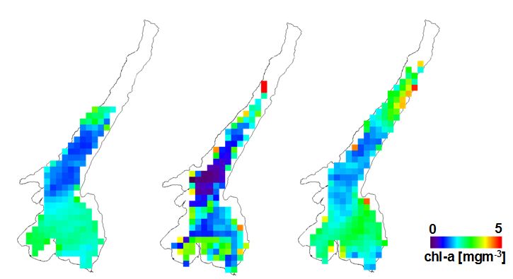
1. Introduction
    In lakes at temperate latitudes the plankton community evolves in an an-
nually recurring pattern [26], with the abrupt onset of phytoplankton growth
in spring as a starting point. The timing of the onset of the phytoplankton
growth is controlled predominantly by abiotic factors such as vertical mixing
and variations in solar radiation [1]. In deep lakes, interannual variations in
the timing of these blooms dominantly result from changes in vertical mixing
rather than solar variations and temperature [20].
    Lake Garda (45 ◦ 40’ N and 10 ◦ 41’ E) is a deep lake with relatively low
concentration of chlorophyll-a (chl-a) and therefore can be classified as an
oligo-mesotrophic basin [5]. With a surface area of 368 km2 it is the largest
fresh water lake in Italy. Lake Garda has a mean depth of 133 m, a maximum
depth of 350 m and a total volume of 49 million m3 . The concentration of
chl-a in Lake Garda ranges from 0.5 to 12 mg m−3 [5].
    It was shown that external factors, such as winter air temperature, spring
lake temperature and extent of surface nutrient enrichment, had significant
effects on the phytoplankton distributions in Lake Garda over the period
1990-2003 [24]. During this period, three complete overturns occurred fol-
lowing harsh winters (1991, 1999 and 2000) associated with increased mixed
layers depths. These overturns, by bringing nutrients to surface layers, deter-
mined different transient effects on several phytoplankton groups with peaks
of different groups at different times within the period from April to August.
    Climate change is unequivocally connected to an increase in surface tem-
perature over lakes in Western Europe, such as the relatively large Lake
Garda. Increased temperatures will affect upper lake temperatures and ther-
mal stratification and hence are expected to change mixing conditions. Cli-
mate warming may therefore induce a shift in the timing and onset of the
growth of phytoplankton and hence strongly affect food-web interactions with
zooplankton and fish [25]. It is therefore important to understand the de-
tailed causal chain between climate change, changes in vertical mixing and
the timing and extent of phytoplankton blooms.
    In this paper, we report on first direct measurements of turbulence char-
acteristics at 4 locations in the southern part of Lake Garda using a SCAMP
(Self Contained Autonomous Microstructure Profiler) during March 5-7, 2014.
From the SCAMP data, profiles of the kinetic energy dissipation ε, the ther-
mal variance dissipation χ and the vertical mixing coefficient KT were de-
termined. Using the fluorometer of the SCAMP, also the vertical profile of

                                      2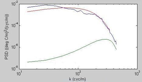
fluorescence is measured.
    Together with data of meteorological forcing (source: MeteoSwiss (high
resolution model COSMO-2)F), nutrient concentrations (water samples) and
remote sensing data (MODIS AQUA), we aim to make a preliminary assess-
ment of the connection between the diurnal variations of vertical mixing and
upper layer chl-a concentrations. In section 2, an overview is provided of the
field measurements with the SCAMP, the additional data obtained and the
data processing. The main results and analyses are presented in section 3
and a summary and discussion of these results is provided in section 4.

2. Data and Methods
2.1. Field work locations
    The measurements in Lake Garda were carried out over the period of
three days from March 5-7, 2014. Over this period, measurements were done
at 4 different stations. In Fig. 1, a map of the southern part of Lake Garda
is shown where the dots represent the locations of the different stations.
The number of profiles measured with the SCAMP are dependent of the
circumstances of the lake. When a lake is stratified, more measurements are
needed to get reliable results than when a lake is homogeneously mixed where
vertical profiles are more comparable to each other. Another influence is the
weather, during rough weather it is more difficult to obtain good quality
measurements than during quiet weather.
    In Table 1, the coordinates, maximum measured depth and number of
measurements at the different stations are listed. The field trip covered
three days of measurements which were split into a morning (before 13:00)
and an afternoon (after 13:00) set. Measurements at the red and black sta-
tion (Fig. 1) were done in the afternoon and at the blue station only in the
morning. At the green station three measurement sets were taken, the morn-
ing of March 6 and both morning and afternoon of March 7.

2.2. SCAMP measurements
    The SCAMP is a free-falling instrument with a fall speed of approxi-
mately 0.1 m s−1 and a temporal resolution of 100 Hz. This results in a
measurement approximately every millimeter, which is needed for charac-
terizing the small-scale turbulent motions. The SCAMP measures vertical
profiles of temperature, fluorescence and photo-synthetically active radiation

                                      3
Figure 1: Stations (colored dots) where SCAMP measurements were done during
March 5-7 in Lake Garda. The precise locations and details on the number of
profiles can be found in Table 1.
Station Location Max. depth of Number of Date
(Fig. 1) measurement measurements
◦
Blue 45.544 N, 100 m 6 5
10.618◦ E March
Black 45.563◦ N, 100 m 6 5
10.621◦ E March
Red 45.494◦ N, 45 m 8 6
10.567◦ E March
Green 45.524◦ N, 75 m 5+5+8 6 & 7
10.602◦ E March
Table 1: Detailed information about measurement locations in Lake Garda dur-
ing March 5-7, 2014.
4(PAR) of the upper layer in high resolution. The maximum measuring depth
of the SCAMP is 100 m which gives a large enough range for measuring
turbulence in the upper layer of a lake.
The SCAMP measures the vertical temperature profile with 2 fast re-
sponse thermistors and 1 accurate thermistor. The fast sensors have a pre-
cision of 0.05 ◦ C, the more accurate thermistor measures with a precision of
0.02 ◦ C. The depth is measured with a pressure sensor with a precision of
0.5% [10]. The depth channel is used to calculate the free-fall velocity of
the SCAMP. Attached to the top end of the SCAMP there is a PAR sensor.
Above the thermistors there is an inlet where water can flow through the
SCAMP from which the fluorescence is measured. Precision of the fluorom-
eter and PAR sensor measurements are not prescribed. The measurements
of fluorescence are given in volt and have to be calibrated with in-situ or
satellite measurements of chl-a, this is further described in Appendix A. De-
tailed information about the SCAMP can be found at the homepage of PME
(http : //www.pme.com/HT M L%20Docs/Scamp− Home.html).
The SCAMP is provided with MATLAB software with which the mea-
sured profiles are preprocessed before analysis. First, a sharpening, smoothen-
ing, trimming and second-order Butterworth Brick-Wall filter are performed
as described by Fozdar et al. (1985) [4]. Next, the measured profiles are
depth-binned; here one meter bins are chosen because of a trade-off between
having sufficient vertical resolution and good statistical robustness. The fi-
nal temperature profiles consist of one value per bin which is the arithmetic
mean of the values in this bin.
2.3. Determination of turbulence quantities
When the assumption is made that dependent quantities are uniform in
the horizontal and that the temporal mean vertical velocity is zero (w = 0)
[19], the temperature variance equation can be written as
∂ 0 2 ∂T
(T ) = −2(w0 T 0 ) − χ. (1)
∂t ∂z
Here, the first term on the right hand side is the production of thermal
variance by the vertical heat flux. The second term describes the dissipation
of thermal variance by thermal diffusion χ (K 2 s−1 ) and is given by
∂T 0 2
χ = 6κ( ). (2)
∂z
5where κ (m2 s−1 ) is the thermal diffusivity. Assuming that production and
dissipation terms balance when averaged over time [22], the left hand side of
(1) is zero. Using a first order closure for the turbulent heat flux, the vertical
mixing coefficient KT (m2 s−1 ) is found from
−2
∂T χ ∂T
w0 T 0 = −KT → KT = . (3)
∂z 2 ∂z
In the turbulent kinetic energy equation, the relevant quantity is the
dissipation of turbulent kinetic energy, indicated here by ε (m2 s−3 ). To
determine ε, processes at the Batchelor length scale are considered, where
advection and diffusion of heat approximately balance. The Batchelor length
scale (lB ) is given by
2 14
νκ
lB = (4)
ε
where ν is the kinematic viscosity (m2 s−1 ). The Batchelor wavenumber is
the inverse of the Batchelor length scale (kB = 1/lB ) and can be estimated
by fitting a (Batchelor) spectrum to the temperature gradient measurements.
We used the maximum likelihood method developed by Ruddick et al. [22],
which is further explained in Appendix B. When kB is determined, ε can be
estimated by
εsegment = (2πkBsegment )4 νsegment κ2 (5)
Where νsegment is the arithmetic mean of the molecular kinematic viscosity in
the segment and kBsegment is the optimal value of the Batchelor wave number
(in cpm). Dillon et al. (1980) [3] and Oakley et al. (1982) [17] concluded
that ε determined indirectly through Batchelor fitting agrees within a factor
2 with the ε determined using vertical shear velocity fluctuations of the flow
.
2.4. Additional data
During the three day campaign, water samples at different depths (sur-
face, 15 m, 30 m and 45 m) were collected for subsequent laboratory analyses
to determine chl-a and nutrient concentrations chl-a. The concentration of
chl-a was measured according to Lorenzen et al. (1967) [15].
Measurements of surface chl-a concentrations done by MODIS AQUA
can be used to calibrate the SCAMP measurements. The way this data is
6processed from the satellite measurements is further discussed in Appendix
C.
COSMO-2 data, source: MeteoSwiss, is used to evaluate the meteoro-
logical circumstances during the field trip, because of its high spatial and
temporal resolution (1 hour, 2.2 km) it can solve small variations of meteo-
rological variables over the lake. This data is used to calculate meteorological
parameters which are discussed below. The wind stress on the water surface
is calculated with help of
2
τ0 = ρair CD U10 , (6)
where CD is the wind-drag coefficient (1.3∗10−3 ) and U10 (m s−1 ) is the wind
speed measured at a height of 10 meters. The net surface buoyancy flux in
fresh water is determined from
gαQ0
Bt = , (7)
ρs Cpw
where g is the gravitational acceleration (9.81 m s−2 ), α (K −1 ) is the
thermal coefficient of expansion, ρs (kg m3 ) is the water density at atmo-
spheric pressure, Cpw (J kg −1 K −1 ) the specific heat capacity of water and
Q0 (W m−2 ) the net surface heat flux.
3. Results
3.1. Meteorological forcing
In Fig. 2 the wind speed measured during the three different days is
shown.
7Figure 2: Wind speed (at 10 meter) output of COSMO-2 model run (data
obtained from MeteoSwiss) over the 3 measurements days. The average wind
speed is taken over the southern part of lake Garda (45.48 - 45.62 ◦ N, 10.57 -
10.66 ◦ W). The area between the vertical black lines indicates the period where
measurements were done. Figures are plotted against different y-axis.
During the field trip, diurnal variation in the meteorological circum-
stances was observed. In the morning relatively high wind speed and high
waves occurred while in the afternoon wind speed decreased and waves almost
8vanished.
Fig. 3 shows the radiation balance (W m−2 ), Buoyancy flux (W kg −1 )
and wind stress (N m−2 ) during the lake Garda field trip calculated from
COSMO-2 meteorological data output. These quantities allow to assess the
relation between the atmospheric forcing and the turbulence in the mixed
layer (ML). The radiation balance is directed from the lake towards the
atmosphere.
Figure 3: Meteorological circumstances during the lake Garda field trip, output
of COSMO-2 (data obtained from MeteoSwiss). COSMO-2 output is averaged
over the southern part of lake Garda (45.48 - 45.62 ◦ N, 10.57 - 10.66 ◦ W). a)
Radiation balance; net surface heat flux (black), net shortwave heat flux (blue),
net longwave heat flux (red), sensible heat flux (pink), latent heat flux (green). b)
Buoyancy flux (W kg −1 ) (c) Wind stress (N m−2 ) red line indicates the critical
wind stress level for turbulence avoidance discussed in section 3.4.
9During the measurement period the net surface heat flux was directed
from the atmosphere towards to ocean, the buoyancy flux ranges from -
4.3 - 8.3 × 10⁻⁸ W kg −1 . Stabilizing the upper lake during the day and
destabilizing during the night. The surface wind stress ranges from 0.0001
to 0.2598 N m−2 with a large peak in wind speed during the night of March
6.
3.2. Observed vertical profiles
In Fig. 4, vertical temperature profiles are plotted. To take the changing
meteorological circumstances into account, a distinction is made between
measurements in the morning and in the afternoon.
Figure 4: Trimmed-smoothed-sharpened-filtered and binned temperature pro-
files that are station averaged and divided in a morning and afternoon measure-
ment set. Data is discarded when there are less than three data points for a certain
depth. The colors of the lines correspond to the color of the stations as shown in
Fig. 1.
During the day the depth binned station averaged temperature profiles
show an increase in stratification because of heating from the sun and calmer
weather conditions in the afternoon. The measurements done on March 5
show a homogeneously ML with a small sloping profile in the morning, while
in the afternoon a small temperature gradient can be seen around the depth
of 25 meters. On March 6 and 7, morning and afternoon temperature profiles
look similar to each other, but in the afternoon the surface temperature is
10increasing. Maximum measurement depth at March 6 is limited because
measurements were done at the shallow part of lake Garda.
Over the three days a stratification build up is seen in the temperature
profiles measured in the morning with a relatively large temperature gradient
appearing near 30 m depth on March 7. The same also holds for the temper-
ature measurement in the afternoon although the temperature gradients are
less obvious on March 5 and 6. On March 6, no clear temperature gradient
was found because of a limited maximum measuring depth at the measured
station.
Fig. 5 presents the vertical profiles of KT , χ and ε (for all 3 days). Miss-
ing data points (white areas) occur due to an insufficient Batchelor fit. The
Batchelor fit rejection criteria are discussed in Appendix B. The vertical
profiles of the turbulence characteristics show relatively high values in the
morning and lower values in the afternoon. This diurnal variation is associ-
ated with the changing meteorological forcing, in particular the changes in
wind stress.
The KT values have a maximum around the middle of the ML and de-
crease towards the top, where the boundary reduces the size of the turbulent
eddies, and towards the bottom of the ML, where the stability of the water
column reduces turbulent mixing. High values of vertical mixing are found
below the ML in the afternoon of March 5 and in the morning of March 7.
χ is largely affected by thermal stratification and its largest values are found
near the surface. The ε measured on March 6 and 7 have higher values in
the morning than in the afternoon. On March 5 there is no large difference
between the morning and afternoon measurements.
In Fig. 6 (a-c) all the binned values of the turbulence characteristics KT
, χ and ε measured within the ML are plotted. It is chosen to only plot
values measured within the ML because the ML is in direct contact with
the atmosphere and this way the effect of changing meteorological forcing on
turbulence in the ML can be studied.
The depth of the ML is usually determined by the depth at which the
temperature difference with respect to the surface is 0.5◦ C [14]. Yet, in our
case of small temperature gradients this definition is not very useful. To
take the small temperature gradient into account we defined the mixed layer
depth (MLD) as the depth where the temperature deviated 0.11◦ C from the
average temperature over the first 10 meters. The averaging over the first 10
meters was done to avoid a strong influence of relatively high temperatures
at the surface (Fig. 4). The value of 0.11◦ C was chosen out of experience and
11Figure 5: Depth binned turbulence characteristics (KT , χ and ε) measured from
5-7 March. The vertical black lines indicate the difference between the days, the
vertical red lines indicate the difference between morning and afternoon. The
colors on the x axis indicates the station where the measurements were done
similar as in Fig. 1. The small black dots represent the maximum depth of the
measurement.
12produced most reliable results. When there was no MLD found according
to the criterion above, the whole profile was averaged. This is done with
an exception of the twelfth profile where the SCAMP started measuring at
a depth of 39 meters. Again, a distinction is made between measurements
done in the morning (before 13:00) and afternoon (after 13:00) to take into
account the effect of changing wind stress.
13Figure 6: Diurnal variation of (a) KT (m2 s−1 ), (b) χ (K 2 s−1 ) and (c) ε
(m2 s−3 ) in the ML. When morning values (blue) are plotted behind afternoon
(green) values this is indicated by the dark green bars.
In Fig. 6 a-c a shift of the turbulence characteristics is seen where rel-
atively high values of turbulence characteristics occur in the morning and
reduced values in the afternoon. In the ML, the median of KT in the morn-
ing is 5.93×10⁻⁴ m2 s−1 and in the afternoon 3.11×10⁻⁵ m2 s−1 . The median
of χ in the morning is 1.49 × 10⁻⁸ K 2 s−1 and in the afternoon 6.86 × 10⁻¹⁰
14K 2 s−1 . The median of ε in the morning is 9.16 × 10⁻⁸ m2 s−3 and in the
afternoon 3.29 × 10⁻¹⁰ m2 s−3 . The median was chosen because when using
a logarithmic scale mean values are not representative. The relatively high
values during the measurements done in the afternoon of March 5 can be
seen as the rightmost green distribution in Fig. 6c.
According to the Osborn-Cox theory [19], a relationship between the ver-
tical mixing coefficient KT , the turbulent kinetic energy dissipation ε and
the Brunt Väisälä frequency N 2 (s−2 ) is expected to be
ε
KT = Γ , (8)
N2
where Γ ≈ 0.2 is the so-called mixing efficiency. According to Ruddick et
al. (1997) [23] this relation valid in turbulent circumstances (high Reynolds
number). To investigate this relationship, a scatter plot is made between
log(KT ) and log(ε/N 2 ) in Fig. 7a and between log(KT ) and log(N ) in Fig. 7b.
15(a)
(b)
Figure 7: (a) Relation between log(KT ) and log(ε/N 2 ) (b) Relation between
log(KT ) and log(N ). The blue line in both figures is according to the Osborn-Cox
theory.
Data plotted in Fig. 7a and b show strong variation around the theo-
retical blue line. According to theory, a linear relationship exists between
log(KT ) and log( Nε2 ) with a slope of 1 and intersection of the y-axis at y =
log(0.2). The data plotted in Fig. 7a shows a linear regression slope of 0.31
and Γ of 0.0041. When only the data measured in the morning, where the
16circumstances are turbulent, is used to determine the mixing efficiency this
equates to a slope of 0.26 and Γ of 0.011. Mixing efficiency is highly variable
and cannot be described by a constant, values of mixing efficiency found are
in the range of O (10− 2) and O (10− 3), one and two order of magnitudes
smaller than the theoretical value.
3.3. Fluorescence and Chlorophyll-a
Calibration of the measured fluorescence data is done as described in
Appendix B. Using this calibration, all the measured chl-a (µg/L) vertical
profiles are shown in Fig. 8. In the upper layer of lake Garda sufficient light
Figure 8: Chlorophyll-a profiles measured using the SCAMP fluorescence sensor
on 5-7 March. Black lines indicate the difference between the days, red lines
indicate the difference between morning and afternoon. The colors on the x-axis
indicate the station where the measurements were done similar as in Fig. 1.
is present for phytoplankton to grow, the euphotic zone. Below the euphotic
zone, because of turbidity of the water and shading by phytoplankton, a
reduced amount of light is limiting phytoplankton growth. Highest concen-
tration of chl-a are found in the middle of the ML, they reduce towards the
surface and the bottom of the ML.
A clear ML is shown in the chl-a distribution with a strong gradient in
the chl-a concentration at the MLD with an exception in the morning of
March 5 where stratification was still weak and mixing to greater depths was
possible.
17During the lake Garda field trip surface chl-a concentrations were mea-
sured by MODIS AQUA. The penetration depth of the remote sensing mea-
surements is dependent on the turbidity of the water column and remains
difficult to determine. As an approximation we assume the penetration depth
to be 10 meters. In Fig. 9 the average concentration of chl-a in the first 10
meters measured by the SCAMP is shown for the three different days. Mea-
surements of MODIS AQUA are plotted at the corresponding time of the
SCAMP measurement. A clear diurnal cycle is visible with relatively low
Figure 9: Chlorophyll-a concentration averaged over the first 10 meter of the
water column measured by the SCAMP. For clarity, the data is divided into three
different days. Black stars represent the chl-a measurements done by MODIS-
AQUA.
concentrations in the morning and increasing concentrations during the day.
In Fig. 8 it can be seen that the high chl-a concentrations in the middle of
the ML spread towards the surface layer during the day. This can be related
to the effect of waves on phytoplankton distribution. The effect of surface
wind stress on vertical phytoplankton distribution is described by (Webster
and Hutchinson et el. (1994) [28]). When the wind speed exceeds a critical
value, phytoplankton is forced down into the water column. Observational
evidence was found by Horne and Wrigly et al. (1975) [9], they found that
wind speeds > 2-3 m s−1 were capable of mixing phytoplankton away from
the water surface. Wind speeds of this magnitude are found at March 5-7 in
the morning and at March 6 in the afternoon (Fig. 2).
18MODIS AQUA measured values at March 5 and 7 are high compared to
values measured with the SCAMP at the same time. At March 6 the chl-a
concentration is too low compared to SCAMP measurement at the same time
but is more on one line with surrounding measurements.
Figure 10 shows maps of chl-a retrieved concentrations measured by
MODIS AQUA after applying BOMBER [7] during the lake Garda field
trip.
Figure 10: The MODIS AQUA-retrieved chl-a mg/L concentrations on March
5, 6 and 7, 2014.
Overall, chl-a concentrations show similar patterns and order of magni-
tude during days of the field trip. Measurements achieved on March 6 show
more patchy patterns with respect to the day before and after, probably due
to the high wind-speed during that day (Fig. 2). In the northern part where
lake Garda is only 3-5 km wide the MODIS AQUA measurements are too
coarse to produce data. Relative high chl-a concentrations are found in the
southern and northern part. In the center concentrations are lower.
In Table 2, the measurements of chl-a based on filtrated water samples
at different depths and surface measurements of MODIS AQUA are listed.
Water samples are used to calibrate the fluorometer of the SCAMP. Assuming
chl-a concentrations are constant in the surface layer surface water samples
are compared with the mean value of the first 5 meters because the SCAMP
19starts measuring at a depth of 2 meter. Satellite surface measurements are
compared by taking the mean value of the first 10 meters of the SCAMP
profile. The correlation between the water surface water samples, MODIS
AQUA and SCAMP measurements at the same time is further discussed
in Appendix A. Also listed are the nutrients N-NO2− + N-NO3− which are
crucial nutrients for phytoplankton growth.
Date Station Depth Sample SCAMP MODIS SCAMP Sample
chlor-a chlor-a chlor-a chlor-a N-NO2 /N-NO3
5-3 blue surf 1.94 0.93 2.19 1.35 414.3
45 m 2.43 2.55 422.8
5-3 black surf 1.26 1.46 1.30 400.3
30 m 1.34 1.38 411.2
6-3 green surf 3.97 1.24 1.44 1.98 379.8
45 m 1.40 1.42 419.2
6-3 red surf 2.44 1.07 2.24 403.9
45 m 2.04 2.31 437.4
7-3 green 15 m 2.60 0.96 2.43 1.33 390.2
45 m 2.25 2.34 394.7
Table 2: Measurements of chl-a and nutrient concentrations (µg/L) during March
5-7 in lake Garda. Comparison of water samples and satellite measurements were
done with SCAMP measurements at the same time and depth. Bolt measurement
depths indicate measurements below the ML in the hypolimnion.
There are four measurements of chl-a and nutrients done below the ML in
the hypolimnion. The concentrations of nutrients N-NO2− and N-NO3− are,
as expected lower, in the ML where nutrients are assimilated by phytoplank-
ton and stratification reduces the supply from below. Between mid autumn
and begin summer nutrient concentrations in the ML are not the limiting
factor for phytoplankton growth. On March 11 silica was measured in the
Northern part of lake Garda (near Brenzone). It is an essential nutrient for
the development of diatoms, and resulted to be above limiting concentration.
Additional measurements of nutrients measured on March 11 are shown in
Appendix D.
3.4. Connection between vertical mixing and chlorophyll-a
The correlation between KT and the chl-a concentration is shown in
Fig. 11. The plotted chl-a concentrations and KT values are the averaged
values in the ML (MLD defined same as in section 3.2).
20Figure 11: Correlation between KT and chl-a in the ML. The colors of the plots
represent the stations where the measurements were done.
A trend is visible in the data: the chl-a concentration decreases when the
vertical mixing coefficient increases. March 5 and 7 show clear trends while
March 6 shows high chl-a concentrations in the morning during high mixing.
Vertical mixing can limit the growth of phytoplankton because of ‘critical
turbulence’; if vertical mixing exceeds a critical value, phytoplankton is mixed
out of the euphotic zone before it had the opportunity to grow and therefore
growth may be reduced [18, 28]. Measurements done on March 11 in the
northern part of lake Garda show that the depth of the euphotic zone is 22
m. At March 5 because of weak stratification phytoplankton is easily mixed
to great depth below the euphotic zone.
High chl-a concentrations measured at March 6 in the morning could be
related to ”turbulence avoidance” by zooplankton. In normal circumstances
zooplankton migrates to the surface at night to eat phytoplankton. In the
excellent summary by Pringle (2007) [21] turbulence avoidance is described
as the migration of zooplankton to deeper layer to avoid Ekman transport at
the surface. Wind stress of 0.0398 to 0.1593 N m−2 are described as sufficient
to drive the turbulent sensitive species out of the Ekman circulation. Wind
stress above this critical value are found at March 6 during the night (Fig.
3c).
214. Summary & Discussion
In this study we have presented in-situ and remote sensing data measured
over three days in the beginning of March at the southern part of lake Garda.
Measurements done at different stations, where differences in circumstances
are small, are compared with each other. Data was obtained by the use of a
free-fall microstructure profiler, water sampling and satellite measurements
done by MODIS AQUA.
During the field trip a diurnal trend in the meteorological forcing was
observed. Where relatively high wind speeds occurred in the morning and
reduced wind speeds in the afternoon. Temperature profiles show a build
up of stratification during the measuring period, the same signal is seen in
measurements of fluorescence.
Measurements of KT , χ and ε done in the ML show a diurnal cycle, high
values of turbulence characteristics are found in the morning and reduced
values in the afternoon. This variation can be related to the diurnal variation
of wind stress induced mixing.
Surface chl-a concentration provided by MODIS AQUA show similar pat-
tern during the field trip. With relative high concentration in the southern
and northern part. Comparison between satellite and SCAMP measurements
remain difficult because of variable maximum penetration depth of MODIS
AQUA.
The correlation between the vertical mixing coefficient and the chl-a con-
centration measured in the ML show a clear trend, this indicates that wind
stress induced mixing is limiting the phytoplankton growth.
Temperature profiles measured at March 5 show homogeneous tempera-
ture profiles where phytoplankton is mixed down to a great depth, indicating
that critical turbulence is limiting phytoplankton growth. Other tempera-
ture profiles show a more stratified profile which reduces the effect of critical
turbulence on chl-a concentrations.
Measurements of high chl-a concentration done at March 6 in the morning
can be related to absence of zooplankton in the night before because of ”tur-
bulence avoidance” [21]. Where zooplankton stays in the deeper parts of the
water column to avoid wind driven Ekman transport. Proof of the absence
of zooplankton could not be provided because zooplankton concentrations
were not measured.
Chl-a surface concentrations increase during the day, this can be related
to wind induced waves which force the phytoplankton down into the water
22column [28]. This is also seen in the chl-a concentrations measured in the first
10 meters of the water column. When there are relatively high wind speeds
the concentration near the surface is relatively low while during reduced wind
speeds the chl-a concentration increases.
The determination of the mixing efficiency on the basis of the Osborn &
Cox relation [19] remain difficult because of the short measurement period
and highly variable turbulence characteristics.
Measurements done in the southern part of lake Garda were done to
gather more knowledge about the effects of vertical mixing on phytoplank-
ton concentration/distribution. These appeared to be the first of turbulence
characteristics in lake Garda. High resolution measurements of fluorescence
distribution show interesting diurnal variation which can be related to dif-
ferent external factors. These results can be used for validation of satellite
chl-a measurements in the upper layer of lake Garda. Hopefully our results
will stimulate further investigation in this field.
235. References
[1] W. Bleiker and F. Schanz. Influence of environmental factors on the
phytoplankton spring bloom in lake zürich. Aquatic Sciences, 51(1):47–
58, 1989.
[2] M. Bresciani, R. Bolpagni, F. Braga, A. Oggioni, and C. Giardino.
Retrospective assessment of macrophytic communities in southern lake
garda (italy) from in situ and mivis (multispectral infrared and visible
imaging spectrometer) data. Journal of Limnology, 71(1):e19, 2012.
[3] T. M. Dillon and D. R. Caldwell. The batchelor spectrum and dissipation
in the upper ocean. Journal of Geophysical Research: Oceans (1978–
2012), 85(C4):1910–1916, 1980.
[4] F. M. Fozdar, G. J. Parkar, and J. Imberger. Matching temperature
and conductivity sensor response characteristics. Journal of Physical
Oceanography, 15(11):1557–1569, 1985.
[5] C. Giardino, V. E. Brando, A. G. Dekker, N. Strömbeck, and G. Can-
diani. Assessment of water quality in lake garda (italy) using hyperion.
Remote Sensing of Environment, 109(2):183–195, 2007.
[6] C. Giardino, G. Candiani, M. Bresciani, M. Bartoli, and L. Pellegrini.
Multi-spectral ir and visible imaging spectrometer (mivis) data to assess
optical properties in shallow waters.
[7] C. Giardino, G. Candiani, M. Bresciani, Z. Lee, S. Gagliano, and
M. Pepe. Bomber: A tool for estimating water quality and bottom prop-
erties from remote sensing images. Computers & Geosciences, 45:313–
318, 2012.
[8] B. Holben, T. Eck, I. Slutsker, D. Tanre, J. Buis, A. Setzer, E. Vermote,
J. Reagan, Y. Kaufman, T. Nakajima, et al. Aeroneta federated in-
strument network and data archive for aerosol characterization. Remote
sensing of environment, 66(1):1–16, 1998.
[9] A. Horne and R. Wrigley. The use of remote sensing to detect how
wind influences planktonic blue-green algal distribution. Verhandlungen
Internationale Vereinigung Limnologie, 19:784–971, 1975.
24[10] E. Jurado, H. van der Woerd, and H. Dijkstra. Microstructure measure-
ments along a quasi-meridional transect in the northeastern atlantic
ocean. Journal of Geophysical Research, 117(C4):C04016, 2012.
[11] S. Y. Kotchenova, E. F. Vermote, R. Matarrese, F. J. Klemm Jr, et al.
Validation of a vector version of the 6s radiative transfer code for at-
mospheric correction of satellite data. part i: Path radiance. Applied
optics, 45(26):6762–6774, 2006.
[12] Z. Lee, K. L. Carder, C. D. Mobley, R. G. Steward, and J. S. Patch. Hy-
perspectral remote sensing for shallow waters. i. a semianalytical model.
Applied Optics, 37(27):6329–6338, 1998.
[13] Z. Lee, K. L. Carder, C. D. Mobley, R. G. Steward, and J. S. Patch. Hy-
perspectral remote sensing for shallow waters. 2. deriving bottom depths
and water properties by optimization. Applied Optics, 38(18):3831–3843,
1999.
[14] S. Levitus, J. I. Antonov, T. P. Boyer, and C. Stephens. Warming of
the world ocean. Science, 287(5461):2225–2229, 2000.
[15] C. J. Lorenzen. Vertical distribution of chlorophyll and phaeo-pigments:
Baja california. In Deep Sea Research and Oceanographic Abstracts,
volume 14, pages 735–745. Elsevier, 1967.
[16] D. A. Luketina and J. Imberger. Determining turbulent kinetic energy
dissipation from batchelor curve fitting. Journal of atmospheric and
oceanic technology, 18(1):100–113, 2001.
[17] N. Oakey. Determination of the rate of dissipation of turbulent energy
from simultaneous temperature and velocity shear microstructure mea-
surements. Journal of Physical Oceanography, 12(3):256–271, 1982.
[18] A. Omta, S. Kooijman, and H. Dijkstra. Critical turbulence revisited:
The impact of submesoscale vertical mixing on plankton patchiness.
Journal of Marine Research, 66(1):61–85, 2008.
[19] T. R. Osborn and C. S. Cox. Oceanic fine structure. Geophysical &
Astrophysical Fluid Dynamics, 3(1):321–345, 1972.
25[20] F. Peeters, D. Straile, A. Lorke, and D. Ollinger. Turbulent mixing and
phytoplankton spring bloom development in a deep lake. Limnology and
Oceanography, 52(1):286–298, 2007.
[21] J. M. Pringle. Turbulence avoidance and the wind-driven transport
of plankton in the surface ekman layer. Continental Shelf Research,
27(5):670–678, 2007.
[22] B. Ruddick, A. Anis, and K. Thompson. Maximum likelihood spectral
fitting: The batchelor spectrum. Journal of Atmospheric and Oceanic
Technology, 17(11):1541–1555, 2000.
[23] B. Ruddick, D. Walsh, and N. Oakey. Variations in apparent mixing effi-
ciency in the north atlantic central water. Journal of Physical Oceanog-
raphy, 27(12):2589–2605, 1997.
[24] N. Salmaso. Effects of climatic fluctuations and vertical mixing on
the interannual trophic variability of lake garda, italy. Limnology and
Oceanography, 50(2):553–565, 2005.
[25] M. Scheffer, D. Straile, E. H. van Nes, and H. Hosper. Climatic warming
causes regime shifts in lake food webs. Limnology and Oceanography,
46(7):1780–1783, 2001.
[26] U. Sommer. Plankton Ecology, succession in plankton communities.
Springer, 1989.
[27] G. I. Taylor. The spectrum of turbulence. Proceedings of the
Royal Society of London. Series A-Mathematical and Physical Sciences,
164(919):476–490, 1938.
[28] I. T. Webster and P. A. Hutchinson. Effect of wind on the distribution
of phytoplankton cells in lakes revisited. Limnology and Oceanography,
39(2):365–373, 1994.
26Appendix A: Calibration of SCAMP fluorometer data
The SCAMP measures fluorescence in voltages and is supplied uncal-
ibrated by PME. Calibration is done by taking water samples at several
depths using a Van Dorne bottle. During the Lake Garda field trip 5 sam-
ples are taken at the surface and 6 at a greater depth (table 2). The samples
taken at the surface are not used for calibration because the SCAMP starts
measuring at a depth of 2 meters. Because the uncertainty of the depth of the
water samples, the two surrounding measured fluorescence segments are also
taken into account. Out of these three values per water sample the values
are chosen which are on one line. This method is an approximation to the
real values and has a large uncertainty. Without the calibration the measure-
ments of fluorescence still provide a qualitative indication of the distribution
of chl-a in the water column.
In Fig. 12 measured chl-a concentrations by the SCAMP and water sam-
ples are plotted. The sample taken on March 6 at a depth of 45 meters in
the afternoon was not used because SCAMP measurements at this station
were not all deep enough.
Figure 12: Correlation between chl-a measurements done by the SCAMP (volt)
and water samples (µg/L).
The conversion factor to convert the SCAMP measurements from voltage
to µg/L out of figure 12 is 4.148.
27Figure 13: Correlation between chl-a measurements by MODIS AQUA (µg/L)
and the SCAMP (volt). For the SCAMP measurements the first 10 meters are
averaged.
The surface chl-a satellite measurements done by MODIS AQUA can also
be used for calibration of the SCAMP fluorometer. Measurements of MODIS
AQUA were done at 12:10, 12:50 and 11:55 UTC. The depth of the satellite
measurements depends on the turbidity of the water and is different for every
profile because of phytoplankton growth and distribution. The assumption
is made that the satellite measures until a depth of 10 meters. The first 10
meters of the SCAMP profile are averaged and compared with the satellite
measurements in figure 13.
Because of the influence of turbidity on the satellite measurements it is
difficult to determine the maximum penetration depth of MODIS AQUA.
Because of the distribution and number of the points shown in Fig. 13 it is
chosen to not use the satellite measurements as calibration for the SCAMP
fluorometer. The conversion factor determined by the in-situ measurements
is used for calibration.
Appendix B: Maximum likelihood Batchelor spectrum fitting
The Batchelor wave number kB can estimated by fitting the observed
temperature spectrum to a theoretical Batchelor spectrum. The observed
vertical temperature profile is divided in segments of 1 meter. By means of
28fast Fourier transform using a hamming window a spectrum of every seg-
ment is made. The observed spectrum is fitted to the theoretical Batchelor
spectrum (equation 9).
Sth (k) = SB (k) + Sn (k) (9)
The theoretical spectrum is built up out of the analytic expression for the
Batchelor spectrum SB (equation 10) and the instrumental noise spectrum
Sn . The magnitude of the noise is different for every SCAMP and can be set
within the MATLAB routine.
1
−1 −1
SB (k; kB , χ) = (q/2) 2 χkB κT f (α) (10)
The non dimensional shape of the spectrum is given by f (α) (equation 11)
where α is the non-dimensional wave number (equation 12) and k is the
wave number (radians/unit length). q is a universal constant range between
3.4-4.1 which is set as 3.4 to match the value used in the SCAMP software
[16].
Z ∞
−α2 /2 −x2 /2
f (α) = α e −α e dx (11)
α
−1
p
α = kkB 2q (12)
In this research we made use of the maximum likelihood estimate (MLE)
(equation 13) to find the best fit between the observed and theoretical spec-
trum. This technique has an explicit incorporation of the instrumental noise.
This offered significant improvement over least square techniques which is
normally used. The best fit between the theoretical and observed spectrum
is found by maximizing C11.
N
X d 2 dSobs (ki )
C11 = ln ∗χ , (13)
i=1
SB (ki ; kB , χθ ) + Sn (ki ) d SB (ki ; kB , χθ ) + Sn (ki )
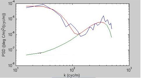
where d is the number of degrees of freedom. An example of a fit between
◦
the spectra is given in figure 14. The power spectral density (( mC )2 / cyc
m
) is
plotted against the wave number (cyc/m).
29Figure 14: Example of a fit between theoretical and observed spectra. The
red line represents the theoretical Batchelor spectrum the blue line the observed
spectrum and the green line the modeled noise.
Some observed temperature gradient spectra can be difficult to fit. When
the wave number is higher instrumental noise becomes more important and
can have an influence on the fit between the spectra. When the amplitude
of the noise is too high comparing the observations this gives a problem
while fitting the theoretical Batchelor shape at the high wave number end.
An other problem can be internal wave and fine-structure contamination at
the low wave number end of the spectra. Because the wave numbers are to
high to fit a theoretical Batchelor spectrum. These limiting Batchelor wave
numbers, which can be used to fit the observations, rely on the range which
can be measured. kL is the lowest wave number at which the Sobs and Sth
intersect and kn is the noisy wave number which depends on the noise of the
SCAMP [16].
To determine if a fit between the observed values and the Batchelor spectrum
is sufficiently good. There are three criteria that the fit should satisfy.
1. Signal-noise ratio; if the integrated signal-noise ratio is smaller than 1.3
the segment is rejected because the level of noise is too high comparing
the signal.
2. The likelihood ratio; in this rejection criteria the Batchelor spectrum
fit (which had a sharp cutoff (fits well for a certain Batchelor wave
number)) is compared with the power law (equation 14) which doesn’t
have a cutoff.
Sth = Ak −b + Sn (14)
30If the Batchelor fit does not provide a significantly better fit than the
powerlaw fit then that segment is rejected because it doesn’t have a
clear cutoff. The two spectral fits are compared by equation 15. If
Lratio is smaller than 2 the segment is rejected. This value is set as 2
out of experience [22].
Batchelorf it
Lratio = log10 (15)
P owerlawf it
3. Variance over the fit; if the variance over the fit is too large the segment
is rejected. The mean absolute deviation is calculated using equation
kn
1 X Sobs Sobs
M AD = − (16)
n k =k Sth Sth
i 1
The value of variance for which a segment is rejected depend on the
degrees of freedom. A segment is rejected when
√
M AD < 2∗ 2∗d (17)
When d is higher more variance around the Batchelor fit is allowed.
Figure 15 is an example of a bad fit where the theoretical Batchelor spectrum
is fitted to the noise. This is a example of a segment that is rejected by the
rejection criteria listed above.
Figure 15: Example of a bad-fit between theoretical and observed spectra. The
red line represents the theoretical Batchelor spectrum the blue line the observed
spectrum and the green line the modeled noise.
31Batchelor curve fitting can only be used when the Taylor hypothesis of frozen
”frozen turbulence” is valid [27]. The = hypothesis is generally considered
to be valid if variations in the fluctuating velocities are small compared with
the velocity of the SCAMP. The speed of the SCAMP is ideally reasonably
greater than the largest turbulent velocity fluctuations. When the SCAMP
velocity is to high roll-off becomes a problem. The turbulence velocity scales
1
as u ∼ (ε∗L) 3 . In an energetic environment ε is around 10−5 and L is around
0.1. This given a u of 0.01 m s−1 thus 0.1 m s−1 is a good compromise between
sensor roll-off and the Taylor hypothesis [16].
Appendix C: MODIS-aqua corrections
MODIS AQUA (MYD021KM product) Level 1B data were used to assess
chl-a concentrations. Radiance products were corrected for the atmospheric
effect with the 6SV1 code (Second Simulation of a Satellite Signal in the
Solar Spectrum, Vector, version 1) [11]. The code was run with an aerosol
model typical for the Po plan valley; the atmospheric profiles were set ac-
cording to the latitude and the season (i.e. Midlatitude winter). For each
image, the aerosol optical thickness at the time of MODIS overpass was de-
rived from AERONET [8] by interpolating data gathered from the stations
closest to Lake Garda (i.e., Ispra, Venice and Modena). The spectral in-
version procedure BOMBER [7], implementing a four-component bio-optical
model [12],[13], was used to estimate chl-a from MODIS-derived Rrs data.
The bio-optical model parameterisation relies on a comprehensive dataset of
concentrations and optical properties we measured in Lake Garda in recent
years [2],[6]. Such parameterisation has been further updated by integrating
data sampled during the three days campaign presented in this study.
Appendix D: Additional nutrient measurements
Table 3 shows measurements done in the Northern part of lake Garda
near Brenzone four days after the lake Garda field trip.
32Depth N-NO3 (µg/L) N-NH3 (µg/L) SiO2 (mg/L)
0 337,24 5 1,14
10 331,41 5 1,15
20 341,49 5 1,20
60 350,10 5 1,20
100 367,40 5 1,49
Table 3: Measurements of nutrients done at the Northern part of lake Garda
(near Brenzone) at March 11.
Measurements of nutrients are as expected lower than during the lake
Garda field trip because of the increasing depth of lake Garda towards the
North. Nutrient concentrations measured are not limiting phytoplankton
growth.
Acknowledgments
Special thanks to Fiona R. vd Burgt and Erwin Lambert for discussing previous ver-
sions of the article. Without there help this article would not be of the same quality.
We also greatly acknowledge all the members of the student room (2014), in special Leon
Saris, Sharon van Geffen, Lotte de Vos and Sjoerd Janson, for mental support and the
organization of coffee-breaks and outdoor activities when needed. Thanks Henk and Lisa
for support, interesting meetings and the great time we had at lake Garda. Most of all
thanks goes out to the support I got from my mother José and two brothers Aart-Jan &
Jelmer.
33You can also read