An Atmospheric Correction Using High Resolution Numerical Weather Prediction Models for Satellite Borne Single Channel Mid Wavelength and Thermal ...

Article

An Atmospheric Correction Using High Resolution
Numerical Weather Prediction Models for Satellite‐
Borne Single‐Channel Mid‐Wavelength and Thermal
Infrared Imaging Sensors
Hongtak Lee 1,2, Joong‐Sun Won 2 and Wook Park 2,*
 1 Satellite Application Division, Satellite Operation and Application Center, Korea Aerospace Research
 Institute, Daejeon 34133, Korea; leeht@kari.re.kr
 2 Department of Earth System Science, Yonsei University, Seoul 03722, Korea; jswon@yonsei.ac.kr

 * Correspondence: pw1983@yonsei.ac.kr; Tel.: +82‐2123‐2673

 Received: 30 December 2019; Accepted: 4 March 2020; Published: 6 March 2020

 Abstract: This paper presents a single‐channel atmospheric correction method for remotely sensed
 infrared (wavelength of 3–15μm) images with various observation angles. The method is based on
 basic radiative transfer equations with a simple absorption‐focused regression model to calculate
 the optical thickness of each atmospheric layer. By employing a simple regression model and re‐
 organization of atmospheric profiles by considering viewing geometry, the proposed method
 conducts atmospheric correction at every pixel of a numerical weather prediction model in a single
 step calculation. The Visible Infrared Imaging Radiometer Suite (VIIRS) imaging channel (375m) I4
 (3.55~3.93μm) and I5 (10.50~12.40μm) bands were used as mid‐wavelength and thermal infrared
 images to demonstrate the effectiveness of the proposed single‐channel atmospheric correction
 method. The estimated sea surface temperatures (SSTs) obtained by the proposed method with high
 resolution numerical weather prediction models were compared with sea‐truth temperature data
 from ocean buoys, multichannel‐based SST products from VIIRS/MODIS, and results from
 MODerate resolution atmospheric TRANsmission 5 (MODTRAN 5), for validation. High resolution
 (1.5km and 12km) numerical weather prediction (NWP) models distributed by the Korea
 Meteorological Administration (KMA) were employed as input atmospheric data. Nighttime SST
 estimations with the I4 band showed a root mean squared error (RMSE) of 0.95℃, similar to that of
 the VIIRS product (RMSE: 0.92℃) and lower than that of the MODIS product (RMSE: 1.74℃), while
 estimations with the I5 band showed an RMSE of 1.81℃. RMSEs from MODTRAN simulations were
 similar (within 0.2℃) to those of the proposed method (I4: 0.81℃, I5: 1.67℃). These results
 demonstrated the competitive performance of a regression‐based method using high‐resolution
 numerical weather prediction (NWP) models for atmospheric correction of single‐channel infrared
 imaging sensors.

 Keywords: mid‐wavelength and thermal infrared; single‐channel atmospheric correction;
 numerical weather prediction model; VIIRS; sea surface temperature

1. Introduction
 Earth surface applications of mid‐wavelength (3–5μm) and thermal infrared (8–14μm) (MWIR
and TIR, respectively) remote sensing, including surface temperature retrieval, essentially require
atmospheric correction. The commonly used methods of atmospheric correction of infrared (IR)
images can be categorized as single‐ or multi‐channel, based on the number of used spectral bands
[1–5]. Currently, most land surface temperature and sea surface temperature (LST and SST,

Remote Sens. 2020, 12, 853; doi:10.3390/rs12050853 www.mdpi.com/journal/remotesensing

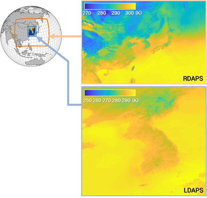
Remote Sens. 2020, 12, 853 2 of 20

respectively) products are based on multichannel methods. The split‐window (SW) algorithm is
widely used for TIR sensors, as it is easy to apply and can be used without extensive computation of
radiative transfer models (RTMs) or explicit information of atmospheric conditions [1,6–9]. However,
these multi‐channel methods have limited application in other types of single‐channel‐based IR
sensors, such as LANDSAT‐7 [10].
 Conventional single‐channel atmospheric correction methods are based on radiative transfer
codes or regression models; those require ancillary atmospheric data such as atmospheric profiles,
total column precipitable water vapor contents (TPW), and near‐surface air temperature [2, 4, 11–13].
Some recent studies used numerical weather prediction (NWP) models as input atmospheric
information for single‐channel atmospheric corrections [14–17]. However, most conventional single‐
channel methods calculate a single set of atmospheric correction parameters (atmospheric upwelling
and downwelling radiances and transmittance) per calculation [7,18]. Depending on the radiative
transfer models, the number of calculations should be increased, or even require calculations for
every pixels of NWP data, in order to minimize the effects of different viewing angles, as well as
atmospheric spatial inhomogeneity and to obtain a uniform atmospheric correction quality within a
scene.
 In this study, we provide an idea of a single‐channel atmospheric correction method, with a
combination of high‐resolution (1.5km and 12km) NWP models from the Korea Meteorological
Administration (KMA). By adopting a simple regression method derived from MODTRAN 5
simulations, the proposed method could calculate atmospheric correction parameters at every pixel
of NWP model data with a single step calculation of the atmospheric correction process by
considering target to sensor geometry.
 The proposed method was applied to the VIIRS imaging channels I4 (3.55~3.93μm, mid‐
wavelength Infrared, MWIR) and I5 (10.50~12.40μm, thermal infrared, TIR) for sea surface
temperature (SST) estimations and a performance verification of the proposed method using the SST
estimation results. Both channels have spatial resolutions of 375 m and 0.4 K of on‐orbit noise
equivalent differential temperature (NEdT) performance [18]. VIIRS imagery was selected because it
has both MWIR and TIR channels within its imaging channels, and its multi‐channel‐based SST
product can be compared with the results of the proposed method.
 The accuracy assessment was conducted by comparing the results with current SST products
(from VIIRS and MODIS), SST estimation using MODTRAN 5 simulations, and sea‐truth data from
ocean buoys in coastal regions of the Korean Peninsula.

2. Materials and Methods

2.1. Numerical Weather Prediction Models
 The Korea Meteorological Administration (KMA) has been producing NWPs with different
spatial resolutions and cover areas. Two models were used in this study: Regional Data Assimilation
and Prediction System (RDAPS) and Local Data Assimilation and Prediction System (LDAPS).
RDAPS covers eastern Asia including Korea, Japan, China, and a part of Southeast Asia with a spatial
resolution of 12km. It analyzes atmospheric conditions four times a day (00, 06, 12, 18 UTC) and
produces 30 weather predictions from +0 h to +87 h with a 3 h interval [19]. LDAPS covers the Korean
Peninsula with a 1.5 km spatial resolution. Its analysis interval is 3 h (00, 03, 06, 09, 12, 15, 18, 21 UTC),
and weather predictions are made at hourly intervals [19] (Figure 1). Twenty six atmospheric layers
were extracted from both models: a 1.5 m geometric altitude layer and 25 isobaric layers from 1000hpa
to 50hpa. Atmospheric temperature, pressure, relative humidity, and geopotential height were used
in this study.

Remote Sens. 2020, 12, 853 3 of 20

 Figure 1. Areal coverage and examples of numerical weather prediction models of Regional Data
 Assimilation and Prediction System (RDAPS) and Local Data Assimilation and Prediction System
 (LDAPS). Examples of atmospheric temperatures at 1.5 m geometric altitude layers, analyzed 4
 September 2014, 18:00 UTC and +0 h prediction. The data and coverage map were obtained from the
 Korea Meteorological Administration (KMA) National Meteorological Super Computer Center [19].

2.2. Formulation of a Regression Model
 To maintain simplicity, the single‐channel atmospheric correction algorithm proposed in this
study was based on the following basic atmospheric radiative transfer equations [20,21]:

 ⁄
 dτ′ (1)
 I ,↑, B T e
 μ

 dτ′ (2)
 I ,↓, B T e
 μ

 T exp τ /μ (3)

where ,↑, is the spectral atmospheric upwelling radiance measured at the top of the
atmosphere (TOA) and I ,↓, is the spectral atmospheric downwelling radiance measured at the
Earth’s surface. Both atmospheric radiances can be calculated by integrations from optical thickness
of TOA level (τ = 0) to that of the Earth’s surface (τ ), with a consideration of light path
geometry (μ, cosine of path zenith angle).
 B is Planck’s function acting as a source function under the local thermal equilibrium condition.
T is the spectral atmospheric transmittance for a total radiation path from the surface to the TOA.
Unlike other variables in Equations (1) to (3), optical thickness can neither be easily acquired from
NWP data, nor simply calculated. Therefore, a regression model was formulated for calculating the
optical thickness. Under clear‐sky conditions with low aerosol content, the scattering process of

Remote Sens. 2020, 12, 853 4 of 20

atmospheric molecules in the 3–15μm infrared region is not as significant as that in shorter
wavelength regions [20–23]. For satellite remote sensing applications upon the Earth’s surface with
clear‐sky conditions, those exclude cloud/fog/aerosol contaminated images. Therefore, to maintain
simplicity, the regression model was focused only on an absorption process in this study.
 An optical thickness between altitudes and could be calculated by Equation (4), without
considering the scattering process.

 , (4)

Here, is an absorption coefficient for wavelength , and is the density of atmospheric
molecules that contribute to the absorption process. With multiple gas species, an absorption
coefficient can be expressed as a summation of the absorption lines of the gas species for the
center wavelength with the strength function and the line shape function , , , given by
Equation (5) [20,22].

 (5)
 , , , , 

 Since Equation (5) is a simple summation, the absorption coefficient can be separated into terms
of dry air, , , and water vapor, , :

 (6)
 , , , , , , , , , ,

 Dividing the absorption coefficients and pre‐calculating coefficients according to infrared
sensors have been attempted in previous studies [24]. In this study, however, an exponential function
was employed to increase the simplicity of the regression model and minimize pre‐calculation while
utilizing NWP models and obtaining 3D atmospheric information from the models [20].
 (7)
 , 
 
Here, an absorption coefficient can be expressed as a function of atmospheric pressure, , and
temperature, . , is the coefficient acquired under reference conditions with pressure,
 , and temperature, . and are exponential terms for pressure and temperature,
respectively, and their values are discussed with Figure 3. Therefore, the atmospheric absorption
introduced in Equation (5) can be expressed as Equation (8), by combining Equations (6) and (7).
 , ,
 
 , , 
 
 (8)
 , , 
 
 The optical thickness can then be calculated with integrations of exponential functions by
substituting Equation (8) into Equation (4).
 , , , 

 (9)
 , , , 
 
 , , , 
 

Remote Sens. 2020, 12, 853 5 of 20

 The integrations in Equation (9) can be solved through a multivariate regression analysis, in
which the two integration terms are considered as two independent variables ( , ), and the dry air
and water vapor reference absorption coefficients , , and , , were used
as the regression coefficients ( , , respectively).
 , ≡ (10)

 Since the reference absorption coefficients become regression coefficients, arbitrary values of
 and can be used. These values were set as 1013 hpa and 290 K, respectively, following
typical ambient atmospheric pressure and temperature conditions. Instead of the 1st order polynomial
regression model of Equation (10), a 3rd order polynomial is practically a more realistic regression
model, as given by Equation (11).
 , ≡ (11)

 In the proposed 3rd order polynomials, the strict physical meanings of the regression coefficients
as the reference absorption coefficients are loosened. However, the 3rd order polynomials are
generally a better fit to the actual atmospheric conditions as compared to the 1st order polynomials.
Thus, Equation (11) was adopted in this study instead of Equation (10) in order to provide
atmospheric optical thickness values and the solution for Equations (1) to (3).

2.3. Determination of Model Parameters
 A normal equation was employed to determine regression parameters.
 θ ̂
 ℎ , ̂ , , , , ⋯ , ,
 1 
 ⎡ ⎤ (12)
 ⎢1 ⎥
 ⎢⋮ ⋮ ⋮ ⋮ ⋮ ⋮ ⋮ ⋮ ⋮ ⋮ ⎥
 ⎣1 ⎦
 θ 
 An observation vector, ̂ , is the optical thickness obtained during the MODTRAN 5 simulation,
and the variables , are calculated from the atmospheric profile used for the simulation
(Figure 2). A total of 520 MODTRAN simulations were conducted to gain values for an observation
vector. A total of 26 atmospheric columns were used, with two profiles per month and one extra
profile for August and January. A total of 20 sensor altitude settings were applied to the atmospheric
profiles, from 0km to 19km with an interval of one kilometer.

Remote Sens. 2020, 12, 853 6 of 20

 Figure 2. A schematic diagram for the simulation of atmospheric layers with multiple sensor altitudes
 and conditions.

 After the calculation of regression coefficients, the least‐squares of ̂ ′ can easily be obtained by:
 ̂ Xθ (13)

 Regression analysis, using Equations (12) and (13), was conducted with various combinations of
exponent terms and from Equations (7) and (8). The combination that resulted in the best fit
model was used for the final calculation of the coefficient P . Figure 3 shows the distributions of
RMSEs calculated from the observation vector and least‐squares fitted values according to the
combinations of the exponent terms and minimum RMSEs.

 (a) (b)

Remote Sens. 2020, 12, 853 7 of 20

 (c) (d)

 Figure 3. Distributions of RMSEs calculated from the observation vector and fitted values according
 to various combinations of exponent terms used for the regression analysis: (a) 1st order regression
 for the VIIRS I4 band (MWIR) and (b) 1st order regression for the VIIRS I5 band (TIR); (c) 3rd order
 regression for the VIIRS I4 band (MWIR) and (d) 3rd order regression for the VIIRS I5 band (TIR). The
 suggested values of and nT were 1 and 0.5, respectively [20]. However, Figure 3 implies that the
 best fit results were obtained at a point different from (1, 0.5). Additionally, the minimum RMSEs of
 the 3rd order polynomial regressions were smaller than those of the 1st order polynomial regression,
 suggesting that the fits of the former are better. The optimal regression coefficients obtained in this
 study for infrared satellite systems are summarized in Table 1.

 Table 1. Regression coefficients used for the infrared satellite systems.

 P0 P1 P2 P3 P4
 System
 P5 P6 P7 P8 P9
 VIIRS I4 0.00148 0.795 0.000499 −0.528 −0.00294
 (MWIR) 0.00000912 0.409 −0.000928 0.0000285 −0.0000000671

 VIIRS I5 0.0318 2.78 −0.00497 4.79 −0.0585
 (TIR) 0.000147 −4.43 −0.00511 0.000497 −0.00000116

2.4. Corrections of Model Biases
 By applying the proposed regression model for the optical thickness (Equation 11, Table 1) and
radiative transfer equations (Equations 1~3), preliminary calculations of the atmospheric correction
parameters via the radiative transfer equations were conducted. Figures 4 and 5 display comparisons
between the preliminary calculation results and simulation results from MODTRAN 5, under a nadir
observation condition. Comparisons before and after model bias corrections under a nadir
observation condition are both provided in the following Figures 4 and 5.

Remote Sens. 2020, 12, 853 8 of 20

 (a) (b)

 (c) (d)

 (e) (f)

 Figure 4. Comparison of the atmospheric correction parameters between the results calculated from
 the proposed regression model with radiative transfer equations and simulation results from
 MODTRAN 5, under a nadir observation condition (VIIRS I4 band): (a, c, e) before correcting for
 model biases; (b, d, f) after correcting for model biases.

Remote Sens. 2020, 12, 853 9 of 20

 (a) (b)

 (c) (d)

 (e) (f)

 Figure 5. Comparison of the atmospheric correction parameters between the results calculated from
 the proposed regression model with radiative transfer equations and simulation results from
 MODTRAN 5, under nadir observation conditions: (a, c, e) before correcting for model biases; (b, d,
 f) after correcting for model biases.

 The model biases could be corrected by matching preliminary calculation results to the
MODTRAN 5 simulated results, with a polynomial regression. Model bias correction functions for

Remote Sens. 2020, 12, 853 10 of 20

VIIRS I4 and I5 bands are listed in Equations (14) to (16). As seen in Figures 4 and 5, the model bias
of atmospheric downwelling radiances was significant for both VIIRS I4 and I5 bands, while that of
the atmospheric transmittance values was relatively insignificant. The atmospheric transmittance
could be directly calculated from optical thickness values with the proposed regression model in
Equation (11). On the other hand, only path radiance and extinction were considered in the
calculation of atmospheric radiances. Therefore, ground/near‐ground multiple scattering could
contribute to the model biases when calculating downwelling radiance between the proposed model
and the MODTRAN. In order to simplify this process, the effects of the ground/near ground multiple
scattering were treated as model bias and corrected with regression models (Figures 4e, 5e).
 0.9875 2.595 3.255 0.6478 4 , 
 T 1.187 2.852 2.572 2.045 0.1528 5 , 
 ℎ , T (14)

 0.4563 0.8519 0.865 0.0005 4 , 
 I ,↑, 0.004 0.0499 0.820 0.0877 5 , 
 (15)
 ℎ , I ,↑, .

 30.45 4.615 1.67 0.001 4 , 
 I ,↓, 0.004 0.0949 1.686 0.0198 5 , 
 (16)
 ℎ , I ,↓, .

 As shown in Figures 4b and 5b, the RMSEs were significantly reduced after the model bias
correction. Figure 6 shows examples of calculated atmospheric downwelling radiances after
correcting for the model bias, compared to MODTRAN 5 simulation results under various
observation angles. The two results were linearly correlated without any offsets, implying that model
biases were successfully separated from the effects of observation angles. Correction functions for
these effects are listed in Equations (17) to (19).

 (a) (b)

 Figure 6. Comparison of the atmospheric downwelling radiances (W/m2/sr/μm) between the
 proposed regression model after the model bias correction and the simulated results of MODTRAN
 5, under various observation angles: (a) for the VIIRS I4 band; (b) for the VIIRS I5 band.

 1.001 0.07362 1.35 1.574 4 , 
 (17)
 , 0.1415 1.25 1.558 5 , 
 ℎ , 

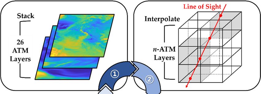
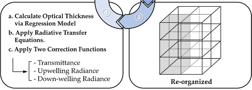
Remote Sens. 2020, 12, 853 11 of 20

 1/ 1.005 0.09463 1.35 1.498 4 , 
 (18)
 , 1/ 1.002 0.1898 1.15 1.553 5 , 
 ℎ , 

 0.9994 0.0172 1.538 4 , 
 (19)
 , 1.001 0.01257 1.58 5 , 
 ℎ , 
where is the observation zenith angle.
 The effects from observation angles can be corrected by multiplying slopes according to
observation angles. An example of acquiring atmospheric transmittance is shown below (Equation
20), where T , , is a result after two steps of correction functions.
 T , , , T (20)

2.5. Processing Steps
 Processing of the proposed single‐channel atmospheric correction method consisted of four
steps: stacking atmospheric layers into 3D cubes, interpolating the layers, re‐organizing atmospheric
blocks according to the observation geometry, and calculating atmospheric correction parameters
(Figure 7).

 Figure 7. Schematic diagram depicting the proposed single‐channel atmospheric correction method,
 which consists of four steps, including the atmospheric blocks re‐organization procedure to
 accommodate various observation angles.

 First, model surfaces and isobaric surfaces from numerical weather prediction models were
stacked according to their geometric altitudes. The models provided geopotential altitudes.
Therefore, the altitudes were converted as per the following equation [25]:
 EH (21)
 Z Units: m
 E H

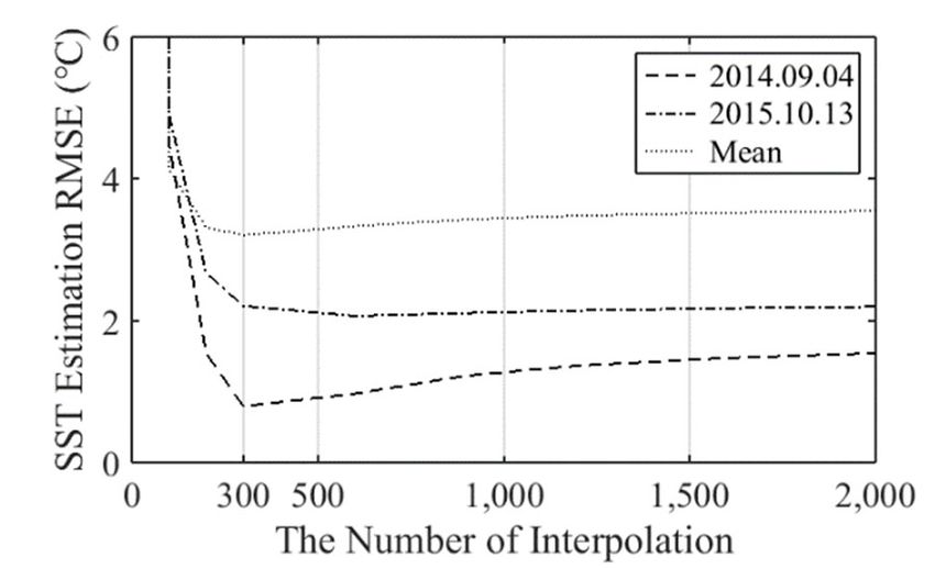
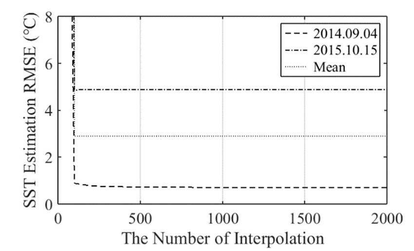
Remote Sens. 2020, 12, 853 12 of 20

where Z is the geometric altitude, H is the geopotential altitude, and E is the radius of the Earth. The
radius was set as 6,371,229 m, following the value assigned by the KMA in the numerical models. In
total, four datasets were stacked: temperature, relative humidity, pressure, and altitude.
 After the altitude unit conversion, the geometric altitudes of each dataset were different. To
conduct re‐organization in Step 3 and to conduct integration in Equations (1) and (2), every dataset
must be in a unified altitude system through an interpolation. Figure 8 shows the variation of average
errors from SST estimations according to the numbers of the interpolated atmospheric layers. In the
figure, as the number of interpolations increases, the average error of the MWIR region decreases.
Even though the decrease after 300 layers was insignificant, atmospheric datasets were interpolated
to 2000 layers for the MWIR region to obtain the best accuracy. For the TIR region, however, the
minimum average error occurred near 300 layers, and therefore, the datasets were interpolated up to
300 layers.

 (a) (b)

 Figure 8. Error patterns of SST estimations according to the numbers of atmospheric layer
 interpolations: (a) absolute values of average errors of SST estimation with VIIRS I4 band (MWIR);
 (b) absolute values of average errors of SST estimation with VIIRS I5 band (TIR).

 After the datasets were interpolated, re‐organization was conducted for each pixel within a
scene, considering the observation geometry of the sensor. Infrared images were assumed to have a
row‐column coordinate system with a north‐up orientation that started from the top‐left corner. Each
pixel on the lowest atmospheric layer was considered as an individual starting point, with row and
column coordinates of r and c , respectively. The following equations were then applied to re‐
organize the atmospheric dataset.

 / (22)

 / (23)

where and are the satellite zenith angle and azimuth angle, respectively, and dz is the
thickness of the atmospheric layer. The result, (r , c ), indicated row‐column coordinates of
pixels on the nth layer and that its value would be relocated to (r , c , n). The re‐organization process
was essential for the proposed algorithm to accommodate various satellite observations and increase
its compatibility. By conducting the re‐organization, calculation over a whole ROI in a vertical
direction with a single process became possible, while considering sensor‐viewing geometry.
 The optical thickness of each atmospheric layers was calculated with the developed regression
model with Equation 11 and the coefficients introduced in Table 1. The calculated atmospheric
thickness was used to acquire the three atmospheric correction parameters (atmospheric up‐/down‐
welling radiances and transmittance) from radiative transfer equations (Eq. 1~3), along with

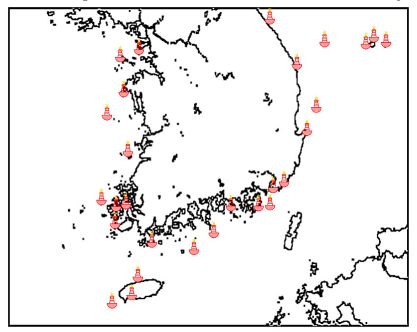
Remote Sens. 2020, 12, 853 13 of 20

atmospheric temperature information from atmospheric profiles. Two‐step correction functions were
applied to remove the model biases of the results.

3. Results and Validations

3.1. Atmospheric Correction Parameters
 The calculated values of atmospheric correction parameters were compared with the simulated
results from MODTRAN 5. The RMSEs according to observation angles are summarized in Table 2.
The parameters were calculated for VIIRS imaging channels I4 and I5 by the single‐channel method
proposed in this study. A total of 24 RDAPS data were randomly selected, and atmospheric profiles
from 28 reference points (Figure 9 and Table 3) were also extracted from each RDAPS data.
 The atmospheric transmittance values with an observation angle of 50 degrees ranged between
0.55–0.9 and 0.2–0.9 for the VIIRS I4 and I5 bands, respectively. The RMSEs of the transmittances
from the proposed method showed 0.6 % (I4 band) and 8 % (I5 band) of their minimum values with
the same observation angle. Under an observation angle of 60 degrees, error levels increased to 2.8 %
(0.4–0.77, I4 band) and 60 % (0.1–0.8, I5 band) of the minimum transmittance values.
 Atmospheric upwelling (I4: 0.005–0.1 and I5: 0.4–6.8 W/m2/sr/m) and downwelling (I4: 0.07–
0.125, I5: 0.4–7.1 W/m2/sr/m) radiances for VIIRS imaging channels had RMSE values less than 2–3
% of their maximum values with an observation angle of 50 degrees. The RMSE levels increased by
up to 60 % as compared to their minimum radiance magnitudes. After the angle was increased to 60
degrees, the RMSEs of upwelling (I4: 0.005–0.14, I5: 0.5–7.5 W/m2/sr/m) and downwelling (I4: 0.005–
0.13, I5: 0.4–6.9 W/m2/sr/m) radiances were less than 4 % of the maximum values and less than 60 %
of the minimum values.

 Table 2. RMSEs of atmospheric correction parameters as compared to MODTRAN 5.

 Systems and
 0˚ 10 ˚ 20 ˚ 30 ˚ 40 ˚ 50 ˚ 60 ˚
 Observation Angles
 
 ,↑, 0.000589 0.000381 0.000429 0.000493 0.000820 0.0014 0.0032

 I4 
 ,↓, 0.000423 0.000410 0.000560 0.000463 0.000759 0.0011 0.0021
 band
 ,↑ 0.0015 0.0012 0.0016 0.0014 0.0033 0.0032 0.011

 ,↑, 0.0863 0.0632 0.0527 0.0599 0.0822 0.0720 0.262

 I5 
 ,↓, 0.0680 0.0604 0.0935 0.0924 0.148 0.216 0.267
 band
 ,↑ 0.00940 0.00710 0.00660 0.00700 0.0128 0.0171 0.0616

3.2. Accuracy of Sea Surface Temperature Estimations

 The proposed single‐channel atmospheric correction method was applied to estimate SST to validate its
 accuracy. Sea surface emissivity values were calculated using a simple model and the ASTER spectral
 library [26,27]. The estimated SST values were compared with sea‐truth temperature data gathered from 28
 buoys, scattered around the southern part of the Korean Peninsula (Figure 9 and Table 3). Those buoys

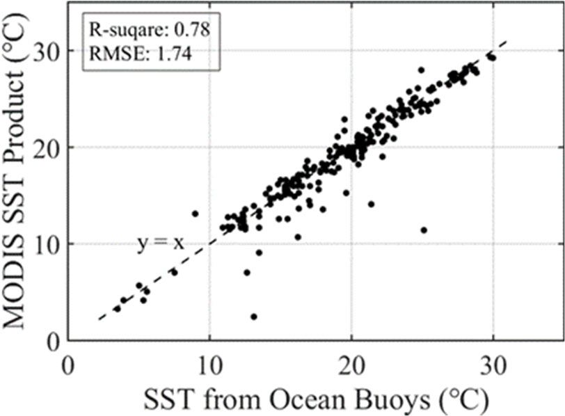
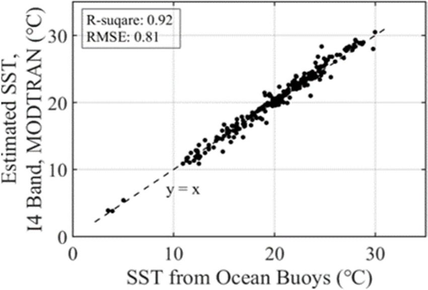
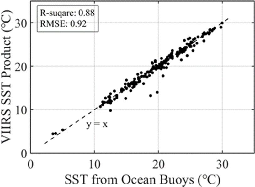
Remote Sens. 2020, 12, 853 14 of 20

 corresponded to the prediction area of the KMA NWP models (Figure 1) [28].

 Figure 9. Distribution of ocean buoys around the southern part of Korean Peninsula, providing sea‐
 truth temperature data for validation.

 Table 3. A list of ocean buoys providing sea‐truth temperature data for validation.

 Locations of Ocean Buoys Employed for Validation

 No. Location Coordinates No. Location Coordinates
 1 Deokjeok‐Do (isl.*) 37°14′10″N/126°01′08″E 15 Cheongsan‐Do (isl.) 34°08′17″N/126°44′39″E
 2 Oeyeon‐Do (isl.) 36°15′00″N/125°45′00″E 16 Geoje‐Do (isl.) 34°46′00″N/128°54′00″E
 3 Seosu‐Do (isl.) 37°19′30″N/126°23′36″E 17 Haeundae 35°08′56″N/129°10′11″E
 4 Sinjin‐Do (isl.) 36°36′18″N/126°07′34″E 18 Dumi‐Do (isl.) 34°44′40″N/128°10′30″E
 5 Chilbal‐Do (isl.) 34°47′36″N/125°46′37″E 19 Haegeumgang 34°44′09″N/128°41′27″E
 6 Chinan 34°44′00″N/126°14′30″E 20 Busan Harbor 35°01′21″N/128°57′22″E
 7 Galmaeyeo 35°36′48″N/126°14′42″E 21 Pohang 36°21′00″N/129°47′00″E
 8 Ock‐Do (isl.) 34°41′34″ N/126°03′20″E 22 Jukbyeon 37°06′15″ N/129°23′22″E
 9 Jin‐Do (isl.) 34°26′33″ N/126°03′25″E 23 Guryongpo 35°59′52″ N/129°35′10″E
 10 Mara‐Do (isl.) 33°05′00″ N/126°02′00″E 24 Ulleung‐Do (isl.) 37°27′20″N/131°06′52″E
 11 Jeju Harbor 33°31′31″N/126°29′38″E 25 Donghae 37°28′50″N/129°57′00″E
 12 Joong Moon 33°13′31″N/126°23′35″E 26 Hyeolam 37°32′29″N/130°51′15″E
 13 Geomun‐Do (isl.) 34°00′05″N/127°30′05″E 27 Goo‐am 37°28′44″N/130°48′16″E
 14 Ganyeoam 34°17′06″N/127°51′28″E 28 Yeongok 37°52′03″N/128°53′08″E
 *isl.: Island

 Three types of remotely sensed SSTs were compared to sea‐truth temperatures obtained from
ocean buoys (Figure 10 and Table 4), which included SSTs computed by the proposed method, a
single‐channel method using MODTRAN 5 simulations for every validation point, and SST products
of VIIRS/MODIS (VIIRS SST Product: VIIRS_NPP‐OSPO‐L2P‐v2.4, MODIS SST Product: MODIS_A‐
JPL‐L2P‐v2014.0) [29,30]. SST estimations using MODTRAN5 were conducted using atmospheric
profiles extracted after the re‐organization process described in Section 2.5, for comparing the results
under similar conditions.
 At night, in the absence of the solar signal, all four errors of the I4 band (mean, Std., Max., RMSE)
were larger while using the proposed single‐channel method than while using the MODTRAN on
the VIIRS I4 band (Table 4). However, their differences were less than 0.2 ℃. RMSE, and the standard
deviation of the I4 band, based on the proposed method, was similar to that of the VIIRS SST product
and half of the MODIS SST product. The maximum absolute error from the proposed method applied
to the I4 band was smaller than that of the VIIRS product. The values obtained for the I4 band using
the proposed method were biased by −0.39 ℃, as shown in Table 4.
 For the I5 band, the proposed method showed the largest RMSE and standard deviation among
the four different SSTs. However, the mean error and maximum absolute error were the smallest at ‐

Remote Sens. 2020, 12, 853 15 of 20

0.07 ℃ and 6.39 ℃, respectively. During the daytime, a mean error of the proposed method using the
I5 band was slightly more than the VIIRS and MODIS SST products. Additionally, standard
deviations of nighttime results showed the MODIS product and the I5 band results with broader
error distributions and larger standard deviations. The VIIRS product and I4 band, which had more
concentrated distributions, showed smaller standard deviations.

 Table 4. Analysis of the estimated SST as derived from VIIRS imaging channels with the proposed
 single‐channel atmospheric correction method, compared with the SST products of VIIRS and MODIS
 based on multichannel atmospheric correction methods.

 Time SST Data Samples Errors (℃)
 Estimated SST, I4 Band, Mean −0.39 RMSE 0.95
 258
 Proposed Std. 0.86 Max. (abs) 3.86
 Estimated SST, I5 Band, Mean −0.07 RMSE 1.81
 258
 Proposed Std. 1.80 Max. (abs) 6.39
 Estimated SST, I4 Band, Mean −0.23 RMSE 0.81
 258
 MODTRAN Std. 0.78 Max. (abs) 3.66
 Night
 Estimated SST, I5 Band, Mean 0.91 RMSE 1.67
 258
 MODTRAN Std. 1.40 Max. (abs) 10.7
 Mean 0.06 RMSE 0.92
 VIIRS SST Product* 210
 Std. 0.91 Max. (abs) 5.75
 Mean 0.33 RMSE 1.74
 MODIS SST Product** 215
 Std. 1.75 Max. (abs) 13.6
 Estimated SST, I5 Band, Mean −0.37 RMSE 1.95
 240
 Proposed Std. 1.91 Max. (abs) 6.14
 Mean −0.14 RMSE 1.95
 Day VIIRS SST Product* 179
 Std. 1.94 Max. (abs) 13.5
 Mean −0.02 RMSE 2.62
 MODIS SST Product** 219
 Std. 2.62 Max. (abs) 14.3
 *VIIRS SST Product: VIIRS_NPP‐OSPO‐L2P‐v2.4 [29]

 **MODIS SST Product: MODIS_A‐JPL‐L2P‐v2014.0 [30]

 (a) (b)

Remote Sens. 2020, 12, 853 16 of 20

 (c) (d)

 (e) (f)

 Figure 10. Nighttime sea surface temperature from ocean buoys versus the SST measure by the
 MODTRAN 5, proposed method, and existing SST products. (a) MODIS SST product (MODIS_A‐JPL‐
 L2P‐v2014.0) [30], (b) VIIRS SST product (VIIRS_NPP‐OSPO‐L2P‐v2.4) [29], (c) VIIRS I4 band
 processed by MODTRAN, (d) VIIRS I5 band processed by MODTRAN, (e) VIIRS I4 band processed
 by the proposed method, and (f) VIIRS I5 band processed by the proposed method.

4. Discussions

4.1. Model Validations
 Even though RMSEs compared to the minimum values of the atmospheric correction parameters
were up to 60%, the comparison results in Table 2 suggested that the simplified regression models
were successfully able to provide the parameters with an accuracy comparable to those by
MODTRAN 5. However, the proposed method required further improvements particularly for high‐
observation angle conditions. Actual effects of the parameter calculation errors could be indirectly
recognized by the estimation result of SST estimated. The results of SST estimation showed that that
accuracy of the proposed method was comparable to that of other multi‐channel‐based methods.
Especially, the SST estimation of the proposed method from the MWIR region (VIIRS I4) resulted in
a difference of 0.03 in both the squared correlation coefficient R2 and RMSE, which was comparable
to the multi‐channel method‐based VIIRS SST product (Table 4). The results from the TIR region
(VIIRS I5) showed the largest RMSE, which would be caused by errors in the atmospheric correction
parameter calculations (Table 4). In addition, the results of the MWIR region for the daytime images
were not presented in this study because they were seriously affected by solar irradiance. The

Remote Sens. 2020, 12, 853 17 of 20

daytime MWIR results after a simple Sun‐glint correction process will be introduced in further
studies.

4.2. Effects of Observation Angles
 Figure 11 shows the error in SST estimation by the proposed method according to various
satellite observation angles during the nighttime. The fitted lines indicate their trends. All I4 and I5
derived results in Figure 11a,b had slopes smaller than the 10‐2 order, which was comparable to that
of VIIRS or the MODIS SST product. This clearly demonstrated that the proposed single‐channel
method was free from angular dependency on SST estimation up to a 60° observation angle. This
suggested that the correction functions for angular effects (Equations 17–19) compensated the effects
of observation angles.

 (a) (b)

 (c) (d)

 Figure 11. Error distributions of SST estimations with the proposed method and their trends
 according to various satellite and observation angles: (a) derived from the VIIRS I4 band, (b) derived
 from the VIIRS I5 band, (c) VIIRS SST product, and (d) MODIS SST product [29,30].

4.3. Effects of Selecting Numerical Prediction Models between LDAPS and RDAPS
 The effects of numerical model spatial resolutions were also assessed based on estimated SSTs
(Table 5). Two types of weather prediction models were used, as described in Subsection 2.1,
including the RDAPS with a resolution of 12 km and the LDAPS with a resolution of 1.5 km. The
results are listed in Table 5. Even with a low spatial resolution of 12 km, the estimation errors of the
I4 derived SSTs were comparable to those obtained by using a model of higher spatial resolution. For
instance, RMSE of the I4 band increased from 0.95 ℃ to 0.99℃, while the maximum error decreased
from 3.80℃ to 3.67℃. However, for the TIR region, errors decreased coherently as the spatial
resolution of the numerical model increased, except for the mean error.

Remote Sens. 2020, 12, 853 18 of 20

 Table 5. Errors of SSTs derived from VIIRS imaging channels with the proposed single‐channel
 atmospheric correction method for comparison between different weather prediction models having
 different spatial resolutions.

 Errors (℃) and LDAPS (1.5 km Resolution)
 Systems Mean Std. Max. RMSE
 VIIRS I4 band −0.23 0.96 3.67 0.99
 VIIRS I5 band 0.98 1.01 3.16 1.41
 Errors (℃) and RDAPS (12 km Resolution)
 Systems Mean Std. Max. RMSE
 VIIRS I4 band −0.39 0.86 3.86 0.95
 VIIRS I5 band −0.07 1.80 6.39 1.81
 To cover the area displayed in Figure 9 and Table 3, in total, 1,920,000 pixels (1200 pixels by 1600
pixels) were required for LDAPS data. Meanwhile, only 28,000 pixels (200 pixels by 140 pixels) of
RDAPS data could cover the same area. The calculation time of the proposed model depended on the
number of atmospheric layers, the amount of NWP data, and computing power. For calculations with
2000 atmospheric layers (for MWIR images), it took about 3 h to process using LDAPS data and about
2 h using RDAPS data. With 300 layers (for LWIR images), it took about 30 min using LDAPS data
and about 20 min using RDAPS data. The calculation time of conventional radiative transfer codes
also depended on conditions and simulation settings. However, an assumption of just 0.5 s per
calculation would result in about 4 h, for calculations on every 28,000 pixels in RDAPS data.
Furthermore, calculations using LDAPS data would cost about 267 h.
 Therefore, according to this brief comparison in this study, a consistent improvement of SST
estimation errors could not be recognized, despite a spatial resolution improvement of NWP data
and an increase of the calculation time. This implied that inhomogeneity of atmospheric components
affecting infrared atmospheric correction would be negligible within the 12 km range and over a sea
surface.

5. Conclusions
 This study proposed a single‐channel atmospheric correction algorithm for both mid‐
wavelength and thermal infrared channels. The proposed algorithm utilized high spatial resolution
NWP models for infrared atmospheric correction. It re‐organized atmospheric profiles according to
each pixel of the NWP models within the infrared images, accounting for their viewing geometry.
Therefore, it was applicable to sensors with a wide field of view or sensors with a high maneuver and
various observation angles. It adopted an absorption‐focused regression model and basic radiative
transfer equations to simplify the calculations. This approach could achieve a simple deduction of
atmospheric optical thickness and the calculation of atmospheric correction parameters, and
consequently, the atmospheric correction parameters for every pixel of NWP data could be calculated
with a single step calculation.
 The proposed method was applied to VIIRS I4 and I5 bands for estimating SSTs and its
validation. SSTs estimated around the Korean Peninsula were compared with sea‐truth temperatures
from ocean buoys for validation. SST products of VIIRS and MODIS, which were based on multi‐
channel methods, were also used for comparison.
 From the results of SST estimation, the proposed method applied to satellite infrared images
showed a comparable accuracy to the widely used RTM, MODRAN 5, or even multi‐channel‐based
atmospheric correction algorithms (VIIRS/MODIS SST products) during the nighttime. In addition,
estimation errors were almost independent of observation angles up to 60°. These validation results
supported that the proposed method using high‐resolution NWP models was effectively able to
conduct an atmospheric correction for various observation angles.
 The KMA NWP models used in this study had specific boundaries of data, which restricted the
validation area of the algorithm. Nevertheless, utilization examples of high‐resolution NWP models,

Remote Sens. 2020, 12, 853 19 of 20

combined with a simplified radiative transfer model, were provided under this study. The results
and approach of this study will be a helpful background for studies combining high‐resolution NWP
models and infrared satellite imagery.
Author Contributions: Conceptualization, Lee, H. and Park, W.; methodology, Lee, H.; software, Lee, H.;
validation, Lee, H., Park, W. and Won, J. S.; formal analysis, Lee, H.; investigation, Lee, H. and Park, W.;
resources, Lee, H., Park, W. and Won, J. S.; data curation, Park, W.; writing—original draft preparation, Lee,
H.; writing—review and editing, Lee, H., Park, W. and Won, J. S.; visualization, Lee, H.; supervision, Won, J. S.;
project administration, Park, W.; funding acquisition, Won, J. S. All authors have read and agreed to the
published version of the manuscript.

Funding: This research was funded by the Ministry of Oceans and Fisheries (MOF).

Acknowledgements: This study was supported by “Base research for building a wide integrated surveillance
system of marine territory” funded by the Ministry of Oceans and Fisheries (MOF).

Conflicts of Interest: “The funders had no role in the design of the study; in the collection, analyses, or
interpretation of data; in the writing of the manuscript, or in the decision to publish the results”.

References
1. Wan, Z.; Dozier, J. A generalized split‐window algorithm for retrieving land‐surface temperature from
 space. IEEE Trans. Geosci. Remote Sens. 1996, 34, 892–905.
2. Jiménez‐Muñoz, J.C.; Sobrino, J.A. A generalized single‐channel method for retrieving land surface
 temperature from remote sensing data. J. Geophys. Res.: Atmos. 2003, 108, 4688–4695.
3. Li, F.; Jackson, T.J.; Kustas, W.P.; Schmugge, T.J.; French, A.N.; Cosh, M.H.; Bindlish, R. Deriving land
 surface temperature from Landsat 5 and 7 during SMEX02/SMACEX. Remote Sens. Environ. 2004, 92, 521–
 534.
4. Jiménez‐Muñoz, J.C.; Cristóbal, J.; Sobrino, J.A.; Sòria, G.; Ninyerola, M.; Pons, X. Revision of the single‐
 channel algorithm for land surface temperature retrieval from Landsat thermal‐infrared data. IEEE Trans.
 Geosci. Remote Sens. 2009, 47, 339–349.
5. Tang, H.; Li, Z.L. Quantitative Remote Sensing in Thermal Infrared: Theory and Applications; Springer Science
 & Business Media: Berlin, Germany, 2013; pp. 13–25, 93–135, ISBN 978‐3‐642‐42027‐6.
6. Ulivieri, C.M.M.A.; Castronuovo, M.M.; Francioni, R.; Cardillo, A. A split window algorithm for estimating
 land surface temperature from satellites. Adv. Space Res. 1994, 14, 59–65.
7. Yu, X.; Guo, X.; Wu, Z. Land surface temperature retrieval from Landsat 8 TIRS—Comparison between
 radiative transfer equation‐based method, split window algorithm and single channel method. Remote Sens.
 2014, 6, 9829–9852.
8. Zheng, X.; Li, Z.L.; Nerry, F.; Zhang, X. A new thermal infrared channel configuration for accurate land
 surface temperature retrieval from satellite data. Remote Sens. Environ. 2019, 231, 111216.
9. Zhang, S.; Duan, S.B.; Li, Z.L.; Huang, C.; Wu, H.; Han, X.J.; Gao, M. Improvement of Split‐Window
 Algorithm for Land Surface Temperature Retrieval from Sentinel‐3A SLSTR Data Over Barren Surfaces
 Using ASTER GED Product. Remote Sens. 2019, 11, 3025.
10. Barsi, J.A.; Schott, J.R.; Palluconi, F.D.; Helder, D.L.; Hook, S.J.; Markham, B.L.; Chander, G.; O’Donnell,
 E.M. Landsat TM and ETM+ thermal band calibration. Can. J. Remote Sens. 2003, 29, 141–153.
11. Wang, M.; Zhang, Z.; Hu, T.; Liu, X. A practical single‐channel algorithm for land surface temperature
 retrieval: Application to Landsat series data. J. Geophys. Res.: Atmos. 2019, 124, 299–316.
12. Jiménez‐Muñoz, J.C.; Sobrino, J.A. A single‐channel algorithm for land‐surface temperature retrieval from
 ASTER data. IEEE Geosci. Remote Sens. Lett. 2010, 7, 176–179.
13. Cristóbal, J.; Jiménez‐Muñoz, J.C.; Prakash, A.; Mattar, C.; Skoković, D.; Sobrino, J.A. An Improved Single‐
 Channel Method to Retrieve Land Surface Temperature from the Landsat‐8 Thermal Band. Remote Sens.
 2018, 10, 431.
14. Barsi, J.A.; Barker, J.L. Schott, J.R. An atmospheric correction parameter calculator for a single thermal band
 earth‐sensing instrument. In Proceedings of the IGARSS 2003, Toulouse, France, 21–25 July 2003; IEEE Cat.
 No. 03CH37477; Volume 5, pp. 3014–3016.
15. Srivastava, P.K.; Han, D.; Rico‐Ramirez, M.A.; Bray, M.; Islam, T.; Gupta, M.; Dai, Q. Estimation of land
 surface temperature from atmospherically corrected LANDSAT TM image using 6S and NCEP global
 reanalysis product. Environ. Earth Sci. 2014, 72, 5183–5196.

Remote Sens. 2020, 12, 853 20 of 20

16. Tardy, B.; Rivalland, V.; Huc, M.; Hagolle, O.; Marcq, S.; Boulet, G. A software tool for atmospheric
 correction and surface temperature estimation of Landsat infrared thermal data. Remote Sens. 2016, 8, 696.
17. Islam, T.; Hulley, G.C.; Malakar, N.K.; Radocinski, R.G.; Guillevic, P.C.; Hook, S.J. A physics‐based
 algorithm for the simultaneous retrieval of land surface temperature and emissivity from VIIRS thermal
 infrared data. IEEE Trans. Geosci. Remote Sens. 2017, 55, 563–576.
18. Cao, C.; Xiong, J.; Blonski, S.; Liu, Q.; Urety, S.; Shao, X.; Bai, Y.; Weng, F. Suomi NPP VIIRS sensor data
 record verification, validation, and long‐term performance monitoring. J. Geophys. Res. Atmos. 2013, 118,
 11–664.
19. Korea Meteorological Administration (KMA). Application Manual of Numerical Forecast Data; Korea
 Meteorological Administration (KMA): Seoul, Korea, 2013.
20. Liou, K.N. An Introduction to Atmospheric Radiation, 2nd ed.; Elsevier: Amsterdam, The Netherlands, 2002;
 pp. 116–168, ISBN 978‐0‐12‐451451‐5.
21. Meador, W.E.; Weaver, W.R. Two‐stream approximations to radiative transfer in planetary atmospheres:
 A unified description of existing methods and a new improvement. J. Atmos. Sci. 1980, 37, 630–643.
22. Lee, K.M. Atmospheric Radiation, 1st ed.; Sigma Press: Seoul, Korea, 2000; pp. 23–31, 109–132, ISBN 89‐8445‐
 037‐5.
23. Griffin, M.K.; Hsiao‐hua.; K. B.; Kerekes, J.P. Understanding radiative transfer in the midwave infrared: A
 precursor to full‐spectrum atmospheric compensation. In Algorithms and Technologies for Multispectral,
 Hyperspectral, and Ultraspectral Imagery X. Int. Soc. Opt. Photonics 2004, 5425, 348–357.
24. Saunders, R.; Hocking, J.; Turner, E.; Rayer, P.; Rundle, D.; Brunel, P.; Vidot, J.; Roquet, P.; Matricardi, M.;
 Geer, A.; et al. An update on the RTTOV fast radiative transfer model (currently at version 12). Geosci. Model
 Dev. 2018, 11, 2717–2737.
25. Carmichael, R. Geopotential and Geometric Altitude; Public Domain of Aeronautical Software (PDA): Santa
 Cruz, CA, USA, 2003.
26. Niclòs, R.; Caselles, V.; Valor, E.; Coll, C.; Sanchez, J.M. A simple equation for determining sea surface
 emissivity in the 3–15 μ m region. Int. J. Remote Sens. 2009, 30, 1603–1619.
27. Baldridge, A.M.; Hook, S.J.; Grove, C.I.; Rivera, G. The ASTER Spectral Library Version 2.0. Remote Sens.
 Environ. 2009, 113, 711–715.
28. Korea Meteorological Administration (KMA). Explanation Document of Meteorological Data; Marine Weather
 Buoys, Wave Height Buoys, Marine Light Beacons; Korea Meteorological Administration (KMA): Seoul, Korea,
 2015.
29. NOAA Office of Satellite and Product Operations (OSPO). GHRSST GDS2 Level 2P Global Skin Sea Surface
 Temperature from the Visible Infrared Imaging Radiometer Suite (VIIRS) on the Suomi NPP satellite created by the
 NOAA Advanced Clear‐Sky Processor for Ocean (ACSPO); Ver. 2.4. PO.DAAC, CA, USA, 2015. Available
 online: https://doi.org/10.5067/GHVRS‐2PO03 (accessed on 23 April 2018.).
30. JPL/OBPG/RSMAS. GHRSST Level 2P Global Skin Sea Surface Temperature from the Moderate Resolution
 Imaging Spectroradiometer (MODIS) on the NASA Aqua satellite; Ver. 2014.0. PO.DAAC, CA, USA, 2016.
 Available online: https://doi.org/10.5067/GHMDA‐2PJ02 (accessed on 23 April 2018.).

 © 2020 by the authors. Licensee MDPI, Basel, Switzerland. This article is an open access
 article distributed under the terms and conditions of the Creative Commons Attribution
 (CC BY) license (http://creativecommons.org/licenses/by/4.0/).