TASTE OVER TIME: THE TEMPORAL DYNAMICS OF USER PREFERENCES
←
→
Page content transcription
If your browser does not render page correctly, please read the page content below
TASTE OVER TIME: THE TEMPORAL DYNAMICS OF USER
                               PREFERENCES

 Joshua L. Moore, Shuo Chen, Thorsten Joachims                                                Douglas Turnbull
   Cornell University, Dept. of Computer Science                                  Ithaca College, Dept. of Computer Science
  {jlmo|shuochen|tj}@cs.cornell.edu                                                      dturnbull@ithaca.edu

                            ABSTRACT                                         over time. Based on these findings, we conjecture that
                                                                             these time-dynamic embedding methods provide exciting
We develop temporal embedding models for exploring how                       opportunities for data-driven exploration of musicological
listening preferences of a population develop over time. In                  trends and patterns. To facilitate such research, scalable
particular, we propose time-dynamic probabilistic embed-                     software implementations of our embedding methods are
ding models that incorporate users and songs in a joint Eu-                  available at http://lme.joachims.org.
clidian space in which they gradually change position over
time. Using large-scale Scrobbler data from Last.fm span-
ning a period of 8 years, our models generate trajectories                                    2. RELATED WORK
of how user tastes changed over time, how artists devel-                     Embedding music into a low-dimensional space is useful
oped, and how songs move in the embedded space. This                         for visualization and automatic playlist generation. There
ability to visualize and quantify listening preferences of a                 are numerous existing algorithms, such as Multi-Dimensional
large population of people over a multi-year time period                     Scaling [7] and Local Linear Embedding [4], which have
provides exciting opportunities for data-driven exploration                  been applied to large corpora of songs and artists.
of musicological trends and patterns.                                            Our work is motivated by recent work of Moore et al.
                                                                             [2, 5] and Aizenberg et al. [1] on using historical playlist
                      1. INTRODUCTION                                        data, but we focus on long-term temporal dynamics. This
                                                                             is different from the short-term dynamics considered by
Embedding methods are a class of models that learn posi-                     Aizenberg et al., namely, the time of day of a track play
tions for discrete objects in a metric space. Such models                    by a station. This time dependency is employed to factor
are widely employed in a variety of fields, including nat-                   out the influence of different format blocks at a radio sta-
ural language processing and music information retrieval                     tion based on the time of day (i.e. a college station may
(MIR). In MIR, these methods find use in recommendation                      play classical music from 6 AM to 9 AM and jazz from
and playlist prediction, among other problems. Embed-                        9 AM to noon). In our work, we allow the positions of
ding methods offer advantages in two main aspects. First,                    users or songs to vary smoothly over the long-term, learn-
they are often very easy to interpret: the resulting space                   ing a representation for each three-month time step from
can be easily visualized and inspected in order to explain                   the beginning of 2005 to the end of 2012. Second, both of
the behavior of the model. Second, they can be applied                       these related works focus on automatic playlist prediction.
to discrete objects without features, learning feature repre-                In this paper, we instead use our model as a data analysis
sentations of the objects as part of model training.                         tool to explore long-range trends in the behavior of users,
   In this work, we explore the use of embedding meth-                       songs, and artists.
ods as a tool for identifying trends and patterns in multi-                      Weston et al. [9] use music embedding for a variety of
year listening data of Last.fm users. In particular, we pro-                 MIR tasks including tag prediction and determining song
pose novel time-dynamic embedding models that gener-                         similarity. Their embedding algorithm works by optimiz-
ate trajectories of musical preferences by jointly embed-                    ing a rank-based loss function (e.g., AUC, precision at k)
ding listeners and the songs they play in a single metric                    over training data for a given task. Our work differs from
space. In order to do this, we extend existing probabilis-                   this in that our embedding results from a probabilistic se-
tic playlists models [1, 2] by adding time dynamics, al-                     quence model that is learned from the track histories of
lowing users and songs to change position on a multi-year                    users. In addition, the work by Weston et al. does not at-
scale. By examining these models, we can draw conclu-                        tempt to model the temporal dynamics.
sions about the behavior of listeners and musical artists                        Dror et al. [3] explore the use of temporal dynamics in
                                                                             collaborative filtering for music. However, the use of time
Permission to make digital or hard copies of all or part of this work for    dynamics in their work is mainly restricted to modeling
personal or classroom use is granted without fee provided that copies are    biases for songs and users, which does not permit the visu-
not made or distributed for profit or commercial advantage and that copies   alization and analysis applications enabled by our work.
bear this notice and the full citation on the first page.                        Finally, Shalit et al. [8] applies a dynamic topic model
 c 2013 International Society for Music Information Retrieval.               to audio features of songs for the purpose of modeling and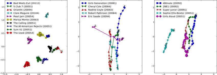
(a)                                             (b)                                                  (c)

Figure 1: Illustrations of the embedding models. Blue dots and red crosses represent songs and users respectively. (a)
Static playlist model. A playlist is represented by songs that are linked by arrows. The next song sne is decided by both
current song scu and the user u (The popularity term also has its effect, which is not shown here). (b) The drifting of a user
u over timesteps in the user-dynamic model. At each timestep, a random walk governed by a Gaussian distribution is taken.
(c) Similar drifting of a song s over timesteps in the song-dynamic model.

discovering musical influence. While this work does not                    probability of a playlist is therefore
explicitly involve embedding songs, users or artists, it is a                                          kp
good example of the use of temporal dynamics in analysis
                                                                                                       Y
                                                                                         Pr(p|u) =           Pr(p[i] |p[i−1] , u).                    (1)
of music data. In addition, their topic model requires audio                                           i=1
features to represent each song. This is in contrast to our
                                                                           Note that transition triples (sne |scu , u) (i.e., reads as “user
model where features are not required.
                                                                           u listened to the current song scu , then listened to the next
                                                                           song sne ”) are a sufficient statistic for this model.
                                                                               Our goal is to embed each song and user into a d-
                           3. MODEL                                        dimensional latent Euclidean space such that song-song
                                                                           and song-user distances model the transition probabilities
In this section we detail the probabilistic embedding mod-
                                                                           Pr(sne |scu , u). This provides such distances with a clear
els we propose for temporal embedding of users and songs.
                                                                           semantic meaning. More specifically, we want to learn a
Starting from a static playlist model (Section 3.1) similar
                                                                           mapping X(·) that maps every song s or user u into that
to [2, 5], we incorporate a macroscopic temporal model
                                                                           space, namely X(s), X(u) ∈ Rd . The dimensionality d
under which the embedding can change over time, pro-
                                                                           is manually specified. Alternatively, X can be considered
viding trajectories for users and songs through embedding
                                                                           as a (|S| + |U|) × d embedding matrix, the rows of which
space. In particular, we propose a user-dynamic embed-
                                                                           correspond to the position of songs and users in the latent
ding model (Section 3.2) in which users move against over
                                                                           space. We will not distinguish the two interpretations of X
a map of songs, as well as a song-dynamic embedding
                                                                           in the rest of the paper if it is clear from the context.
model (Section 3.3) in which songs move against a map
                                                                               The specific model we propose for relating distances to
of users. For both models, we briefly outline how they can
                                                                           transition probabilities is
be trained using maximum likelihood (Section 3.4).
                                                                                                                  2             2
                                                                                                    e−∆(sne ,scu ) −∆(sne ,u)       +bidx(sne )
                                                                               Pr(sne |scu , u) =                                                 ,   (2)
                                                                                                                Z(scu , u)
3.1 Embedding Songs and Users for Playlist Modeling
                                                                           where ∆(x, y) = ||X(x) − X(y)|| is the Euclidean dis-
Given a collection of songs S = {s1 , . . . , s|S| } and a col-            tance between two embedded items (either song or user) in
lection of users U = {u1 , . . . , u|U | }, each user’s listen-            the latent space. bidx(s) is a scalar bias term that is added
ing history can be described as a sequence of songs p =                    to model the popularity of each song, where idx(s) returns
(p[1] , ..., p[kp ] ) of length kp , where each p[i] ∈ S. We refer         the index for song s. For example, idx(si ) = i. Z(scu , u)
to this (multi-year) sequence as the “playlist” of that user.              is the partition function that normalizes the distribution. It
The collection D of all user playlists is the training data                is defined as
for our embedding method.                                                                           |S|
                                                                                                                      2
                                                                                                                          −∆(si ,u)2 +bi
                                                                                                    X
    Following the approach proposed in [2], we model a                              Z(scu , u) =          e−∆(si ,scu )                      .        (3)
user’s playlist using a first-order Markov model, but also                                          i=1

augment it with a user model similar to [1]. As a result,                  Panel (a) of Figure 1 illustrates how song and user posi-
the probability Pr(sne |scu , u) of the next song in a playlist            tions in the embedding space relate to the transition prob-
depends only on the current song and the user. The overall                 ability Pr(sne |scu , u). The red cross is the position of the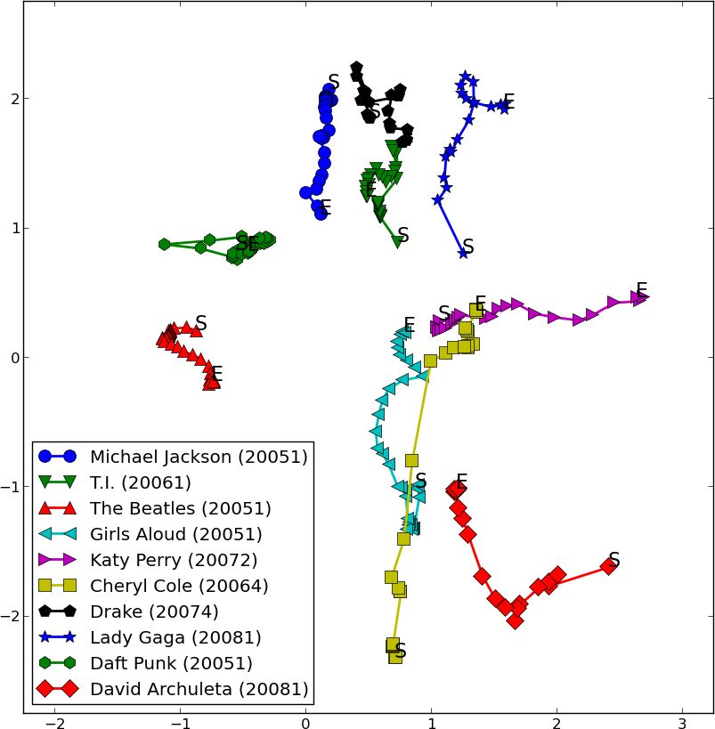
user, and the blue dot labeled scu is the current song in the where the song and time-dependent user positions are opti-
playlist. The probability of playing some song sne next de- mized to maximize the likelihood of the observed playlists.
pends on its sum of the squared distances to the current
song and the user, plus its inherent popularity bsne . This 3.3 Song-dynamic Embedding Model
means that the transition to the next song sne is more likely
Similar to the user-dynamic embedding model, we also
if (1) the next song is close to the current song in the latent
consider a song-dynamic embedding model which fixes the
space, (2) the next song is close to the user(’s taste) in the
position of users and allows songs to drift over time. In this
latent space, or (3) the next song is popular. We focus our
model, the probability of each transition triple is
experiments on two-dimensional embeddings, since this
provides us with an X that can easily be visualized. How- −∆(s(t) (t) 2
(t)
ne ,scu ) −∆(sne ,u) +bidx(s
2 (t)
ever, higher-dimensional embeddings are possible as well. e ne )
Pr(s(t) (t)
ne |scu , u) = (t)
. (6)
Z(scu , u)
3.2 User-dynamic Embedding Model
After introducing an analogous Gaussian random walk for
Combining Equations (1) and (2) models a playlist as songs over different timesteps (as illustrated in Panel (c) of
a stochastic process on a microscopic level (i.e., on the Figure 1), we get the training problem
timescale of minutes). In addition, we also model changes
Y
in user preferences as a stochastic process on a macro- Pr(s(t) (t)
max ne |scu , u)
scopic level. In the following experiments, each macro- X∈R(|T ||S|+|U |)×d
(t) (t)
b∈R|T |×|S| (sne |scu ,u)∈D
scopic timestep t ∈ T (T is the set of all timesteps) de-
|S|
notes a quarter of a year, and notation like 20083 denotes Y Y (t−1) (t) 2
· e−νsong ∆(si ,si )
, (7)
“third quarter of year 2008”.
i=1 t∈{τ |(τ ∈T )
Let us first consider a macroscopic stochastic process ∧(τ −1∈T )}
where positions of users are changing over time, while the
position of the songs are fixed in the latent space. Denot- where users and time-dependent song positions are opti-
ing with u(t) the position of user u in embedding space mized.
at timestep t, the overall trajectory of a user is u(∗) = From a technical perspective, it is conceivable to train
(u(1) , u(2) , ...). At each timestep t, the microscopic transi- an embedding model with both users and songs varying
tion probability Pr(sne |scu , u(t) ) now depends on the users their position over time, which will output an embedding
current position, and the conditional probability of the next matrix X of (|T |(|S| + |U|)) rows. We briefly explored
song is this model, but found it difficult to interpret the resulting
trajectories. We therefore focus on the restricted models in
2 (t)
−∆(sne ,scu )2 −∆(sne ,u(t) ) +bidx(s our empirical evaluation.
(t) e ne )
Pr(sne |scu , u ) = . (4)
Z(scu , u(t) )
3.4 Training of Probabilistic Embedding Models
Note that even though the positions of songs are fixed, we
(t) The maximum likelihood optimization problems in Equa-
still give each song a time-varying popularity term bi .
tions (7) and (5) are of substantial scale. Previous sequence
To restrict users from drifting too much from one
models were trained using stochastic gradient methods
timestep to the other, we model a users trajectory as a
[1, 2, 5]. However, those training algorithm does not scale
Gaussian random walk. Panel (b) of Figure 1 illustrates
well, since the complexity of each training iteration is
such a random walk. Concretely, this means that the user’s
(t−1) quadratic in the number of terms in the partition function
next position u(t) is a Gaussian step N (ui , 2ν1user Id ) (in our case |S|). In related work on (non-temporal) se-
from the current position u(t−1) . Here, Id is the d- quence modeling for natural language [6], we developed
dimensional identity matrix, and νuser is the variance an approximate, sampling-based training algorithm which
(which can be viewed as a regularization coefficient that estimates the partition function on the fly. This training
influences step sizes). This Gaussian distribution makes procedure has complexity which is only linear in the num-
it more likely that the user’s positions at two consecutive ber of terms in the partition function, and we adopt this
timesteps are close to each other. algorithm for training. A software package implement-
Considering both the stochastic process over transition ing the training algorithm is available online at http:
triples and the stochastic process describing the users’ tra- //lme.joachims.org.
jectories, the overall user-dynamic embedding model can
be trained via maximum likelihood. The resulting opti-
4. EXPERIMENTS
mization problem is
Y Our experiments revolve around a Last.fm data set which
max Pr(sne |scu , u(t) ) we crawled using the site’s API 1 . The crawl was con-
X∈R(|S|+|T ||U |)×d
b∈R|T |×|S| (sne |scu ,u(t) )∈D ducted over the course of several weeks in the fourth quar-
|U | ter of 2012. Although it is unused in this work, we were
Y Y (t−1) (t) 2
· e−νuser ∆(ui ,ui )
, (5) initially also interested in the social network data, so we
i=1 t∈{τ |(τ ∈T )
∧(τ −1∈T )} 1 http://www.last.fm/api
Figure 2: The song-dynamic model’s song space plotted (from left to right) at 20051, 20091, and 20124

crawled through the social network using the top listener
for each of the 10 top artists on the site at the time as seeds.
For each user, we crawled the user’s complete timestamped
track history and friends list. We later augmented this data
with the age, gender, and country of each user (for those
for which it was available). We also crawled the tags for
some of the songs, although we do not take advantage of
this data in this work.
   The result contains over 300,000,000 track plays by
roughly 4700 users, with over 550,000 unique tracks. This
data contains many noisy track names, so we pruned the
data further by only considering tracks with at least 1000
plays and discarding users with no remaining track his-
tory after infrequent songs are discarded. This yields
the set of track histories used in the experiments, which
contains 4,551 users, 32,401 unique tracks, and roughly
200,000,000 track plays. We used this to create our “per-
user playlist” data by splitting the track histories into
playlists of consecutive songs that were played within 15
minutes of each other. Finally, we quantized the times-            Figure 3: Artist trajectories over time. The legend gives
tamps to divide each user’s track history into year quarters,      the first quarter in which each artist was observed
ranging from first quarter, 2005 until fourth quarter, 2012,
for a total of 32 timesteps. From this point on, we will refer
                                                                   78% of the users are male, and about 88% are between the
to the nth quarter of year yyyy as yyyyn, such as 20051
                                                                   ages of 15 and 25 (roughly evenly split between the two
for 2005 first quarter.
                                                                   groups) as of the crawl in 20124. The median user age is
   We considered models with 2 dimensions in this work
                                                                   20, and the average is about 20.8. Due to the social net-
for the sake of simplicity and ease of visualization. In or-
                                                                   work crawl and a coincidence of the seed users, roughly
der to find good values for νsong and νuser , we further di-
                                                                   57% of our users are from Brazil. The country distribu-
vided the data by placing each fifth song transition into a
                                                                   tion has a fairly long tail, with only 84% coming from
validation set and the rest into the training set. We then
                                                                   the 10 most popular countries, and 91% coming from the
used these to validate for the optimal values of these pa-
                                                                   20 most popular countries. The ten most well-represented
rameters. The user-dynamic model performed best with a
                                                                   countries in the data set are Brazil (57%), US (8%), UK
low value of νuser , with its optimal value at 0.01. In con-
                                                                   (4%), Poland (3%), Russia (2.6%), Germany (2.3%), Spain
trast, the song-dynamic model performed best with strong
                                                                   (1.6%), Mexico (1.6%), Chile (1.3%), and Turkey (1.1%).
regularization, and the optimal νsong was found to be 2.0.
                                                                   4.2 Song-dynamic Model
4.1 Demographics of users
                                                                   In the song-dynamic model, songs can move over time
The demographics of the data set reflect characteristics of        through a map of users. Among other things, the result-
the average Last.fm user. For each demographic category,           ing trajectories give insight into how the appeal of songs
we report percentages based on the number of users report-         and artists changed over time.
ing in that category. 83% reported an age, 89% reported               In Figure 2, we show the embedding of the songs at the
a country, and 91% reported gender. In our data, about             start, middle, and end of the time sequence (i.e., timesteps
Figure 4: The 10 artists with the smallest variance in position over time (left) and the 10 with the largest variance in position
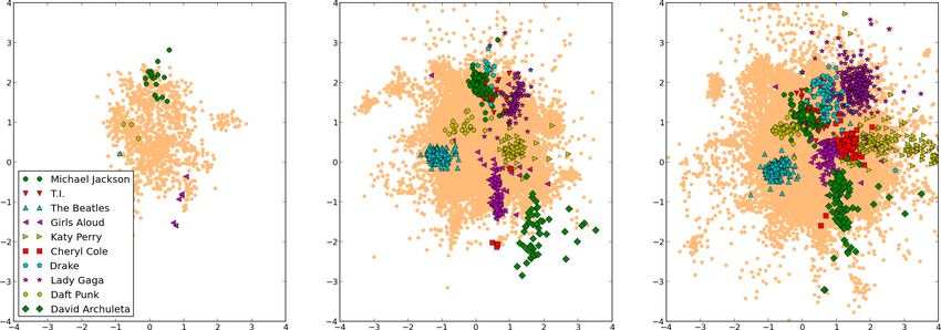
over time (top 5 in center, next five at right). The first timestep at which each artist was observed is listed in parentheses.
20051, 20091, and 20124). A song is plotted once it has Daft Punk also starts to drift away from the center until
been played at least once, which explains why the space the release in December, 2010 of the motion picture Tron:
becomes more dense over time. The locations of users Legacy, which featured a popular soundtrack by the duo.
are not plotted to reduce clutter. Generally speaking, the We can also see Girls Aloud and Cheryl Cole (of Girls
density of users is greatest around the origin and then de- Aloud) drift from the edges rapidly towards the center in
creases outwards. In this sense more popular music lies in correlated paths, and the emergence of David Archuleta, an
the center, but note that we also capture popularity through American Idol runner-up in May, 2008. All follow a sim-
the specific song bias parameter. ilar trajectory in user space, indicating that the users that
previously listened to Girls Aloud are listening to David
Are similar songs embedded at similar locations? To Archuleta a few years later.
illustrate the semantic layout of the embedding space, we We can also see artists like Katy Perry and Lady Gaga
highlight the songs of some reference artists. Note that drift away from the center after the peak of their popular-
the songs of the reference artist cluster even though our ity, and we see Drake drift towards the center in what can
embedding method has no direct information about artists. partly be explained by a shift in his style from something
This verifies that the model can indeed learn about songs more hip hop oriented to a somewhat more poppy style.
similarity merely from the listening patterns. We also
note that our intuitive notion of artist similarity generally What does the variance of a trajectory indicate? The
matches the distance at which our model positions them in trajectories are useful not only for visualization, but also as
embedding space. the basis for further aggregating and quantifying the behav-
ior of an artist. Figure 4 shows the artists with the smallest
How do songs and artists move? Figure 2 also shows and largest variance in position over time. The specific cri-
that the songs of some artists move in the embedding space, terion used here for a given artist is the average distance
while others remain more stationary. The artists’ changes over timesteps from the artist’s embedding at that timestep
are aggregated into trajectories and displayed in Figure 3. to the mean vector of that artist’s representation over all
Each dot in Figure 3 indicates the mean location of the time steps. To avoid obscure artists that would be diffi-
songs of one artist at a specific time step. This plot enables cult to interpret without further background knowledge, we
us to see more clearly some events and trends in the music only consider artists who appeared in the track histories of
world that influence the model. at least 10% of the users.
First, note that Michael Jackson’s trajectory starts off The left-hand panel in Figure 4 shows the 10 artists with
clumped together in the same space, moving very little. small variance. Many of these are well-established artists
Then, after some number of timesteps, it starts moving that probably undergo little change in style or fan base.
quickly towards the center. Upon closer inspection, the The panel in the middle and on the right-hand side of
turning point in this trajectory turns out to line up exactly Figure 4 show the 10 artists with the largest variance. Many
with the death of Michael Jackson in June, 2009. of these are popular artists that have a large change in ap-
Similarly, the Beatles start to drift slightly away from peal – i.e., those that go from being relatively obscure to
the center as many other artists enter the model. Then, they quite popular.
make an abrupt turn back towards the center. This aligns The variance of a trajectory in only one possible statistic
with the release of the Beatles’ full catalog on iTunes in that summarizes a path. We conjecture that other summary
the 20104 after being totally unavailable via digital distri- statistics will highlight other aspects of an artist’s devel-
bution before then. opment, providing additional criteria for exploratory dataover time, which enables the analysis of long-term dynam-
ics of user tastes and artist appeal and style. The ability to
visualize the learned embeddings is a key feature for easy
interpretability and open-ended exploratory data analysis.
We conjecture that such embedding models will provide
interesting tools for analyzing the growing body of listen-
ing data. Furthermore, the embedding models described
in the paper can easily be adapted and extended to include
further information (e.g., social network data), providing
many directions for future work.
5.1 Acknowledgements
This work was supported by NSF grants IIS-1217485, IIS-
1217686, and IIS-1247696. The first author is supported
by an NSF Graduate Research Fellowship. We would also
like to thank the anonymous reviewers for their feedback,
and Brian McFee for helpful discussions and technical ad-
vice.
Figure 5: Trajectories of users with age, grouped by age
in 2005. Each point is labeled with the average age of the
group at that time. The legend also gives the average age 6. REFERENCES
in 2005 of the users in that group (in parentheses). [1] N. Aizenberg, Y. Koren, and O. Somekh. Build your
own music recommender by modeling internet radio
streams. In Proceedings of the 21st international con-
analysis.
ference on World Wide Web, pages 1–10. ACM, 2012.
4.3 User-dynamic model [2] S. Chen, J. L. Moore, D. Turnbull, and T. Joachims.
The user-dynamic model is dual to the song-dynamic model, Playlist prediction via metric embedding. In Proceed-
in that it models trajectories of users on a map of songs. ings of the 18th ACM SIGKDD international confer-
While the trajectories of indiviual users provide an inter- ence on Knowledge discovery and data mining, pages
sting tool for reflection, they are difficult to interpret for 714–722. ACM, 2012.
outsiders. We therefore only show aggregate user paths. [3] G. Dror, N. Koenigstein, and Y. Koren. Yahoo! music
One such aggregation is shown in Figure 5. Here, we recommendations: modeling music ratings with tem-
can see the behavior of users when aggregated by age. poral dynamics and item taxonomy. In Proceedings of
Specifically, the users are grouped by age in 2005 in order the fifth ACM conference on Recommender systems,
to separate the effect of a person’s absolute age from the pages 165–172. ACM, 2011.
effect of the change in the average listener’s taste profile.
Distinctive differences in trajectory can be seen, with [4] V. Jain and L. Saul. Exploratory analysis and visualiza-
the youngest group moving to north, away from Katy Perry tion of speech and music by locally linear embedding.
and many other more “sugary” pop artists, and towards ICASSP, 2004.
more dance and R&B oriented pop artists as well as the
hip hop cluster which is further north, outside the figure. [5] J. L. Moore, S. Chen, T. Joachims, and D. Turnbull.
The other age groups see more lateral moves and tend Learning to embed songs and tags for playlist predic-
to be further north, even when age is fixed. The oldest age tion, 2012.
groups (where 22 to 30 and 31 to 62 were aggregated with a [6] J. L. Moore and T. Joachims. Fast training of proba-
larger interval due to a smaller number of users in these age bilistic sequence embedding models with long-range
ranges) start very far north, and the 31 to 62 group mostly dependencies. Arxiv pre-print, 2013.
hovers around the eastern part of the figure. Outside of the
figure and to the right are where many older rock bands [7] J. Platt. Fast embedding of sparse music similarity
such as the Rolling Stones and the Beatles lie, and this graphs. NIPS, 2004.
oldest age group is also closer to them.
[8] U. Shalit, D. Weinshall, and G. Chechik. Modeling mu-
sical influence with topic models. In ICML, 2013.
5. CONCLUSIONS
[9] J. Weston, S. Bengio, and P. Hamel. Multi-tasking
We presented novel probabilistic embedding methods for
with joint semantic spaces for large-scale music anno-
modeling long-term temporal dynamics of sequence data.
tation and retrieval. Journal of New Music Research,
These models jointly embed users and songs into a met-
40(4):337–348, 2011.
ric space, even when no features are available for either
one. Users and/or songs are allowed to change positionYou can also read