Improved Facial Expression Recognition Based on DWT Feature for Deep CNN - MDPI
←
→
Page content transcription
If your browser does not render page correctly, please read the page content below
electronics
Article
Improved Facial Expression Recognition Based on
DWT Feature for Deep CNN
Ridha Ilyas Bendjillali 1, * , Mohammed Beladgham 1 , Khaled Merit 1 and Abdelmalik
Taleb-Ahmed 2
 1    Laboratory of TIT, Department of Electrical Engineering, Tahri Mohammed University, Bechar 08000,
      Algeria; beladgham.tlm@gmail.com (M.B.); merit1984@gmail.com (K.M.)
 2    Laboratory of IEMN DOAE. UMR CNRS 852, University of Valenciennes, 59313 Valenciennes, France;
      Abdelmalik.Taleb-Ahmed@univ-valenciennes.fr
 *    Correspondence: rayben43@gmail.com

 Received: 18 January 2019; Accepted: 8 March 2019; Published: 15 March 2019

 Abstract: Facial expression recognition (FER) has become one of the most important fields of research
 in pattern recognition. In this paper, we propose a method for the identification of facial expressions
 of people through their emotions. Being robust against illumination changes, this method combines
 four steps: Viola–Jones face detection algorithm, facial image enhancement using contrast limited
 adaptive histogram equalization (CLAHE) algorithm, the discrete wavelet transform (DWT), and
 deep convolutional neural network (CNN). We have used Viola–Jones to locate the face and facial
 parts; the facial image is enhanced using CLAHE; then facial features extraction is done using DWT;
 and finally, the extracted features are used directly to train the CNN network, for the purpose of
 classifying the facial expressions. Our experimental work was performed on the CK+ database and
 JAFFE face database. The results obtained using this network were 96.46% and 98.43%, respectively.

 Keywords: facial expression recognition (FER); deep convolutional neural network (deep CNN);
 discrete wavelet transform (DWT); contrast limited adaptive histogram equalization (CLAHE)

1. Introduction
      Facial recognition is currently the most important biometric identification technology; this
technique has many advantages, such as low cost and high reliability. Facial recognition has been used
in several areas such as pattern recognition, computer vision, security, and cognitive science.
      In recent years, facial expression recognition (FER) techniques aroused more and more interest
on the part of the scientific community [1,2]. Facial expressions are an effective way in human and
computer machine interaction and non-verbal interpersonal communications. It has many different
applications in various fields such as security-surveillance, artificial intelligence, military and police
services, and psychology, among others.
      Facial expressions are classified into six basic categories; namely, anger, disgust, fear, sadness,
happiness, and surprise—a neutral expression was also added to this group.
      Facial expression recognition goes through three main steps. The first is face detection in the image.
Its effectiveness has a direct influence on the performance of the FER system. The second important
step of an FER system is facial features extraction, and the third and last step is expression classification.
      In recent years, a wide variety of facial expression recognition methods have been proposed,
such as elastic bunch graph matching (EBGM) [3], independent component analysis (ICA) [4], linear
discriminant analysis (LDA) [5], principal component analysis (PCA) [6], scale invariant feature
transform (SIFT) [7], and embedded hidden Markov models (EHMM) [8].

Electronics 2019, 8, 324; doi:10.3390/electronics8030324                     www.mdpi.com/journal/electronics
Electronics 2019, 8, 324 2 of 16
These methods have been used to improve the recognition rate and speed of facial expression
recognition, but several challenges are confronted with regard to variations in the person’s pose,
changes in illumination, and so on.
Alternative methods are based on transforms such as Fourier transform (FT), short time FT
(ST-FT), and discrete wavelet transform (DWT) [9]. Feature extraction based on the DWT method
is very useful for FER with very low computational cost, which makes it an ideal tool for image
processing and computer vision.
The main contributions of the proposed methodology are as follows: first, to develop a robust
feature extraction approach; second, to improve the performance of the FER system and obtain a high
recognition rate.
In this paper, we propose a model by applying the Viola–Jones face detection algorithm to detect
faces, and to separate the faces from the rest of the parts considered non-faces. For our application,
we have opted for different types of image enhancement algorithms to improve image contrast, the
evaluation and judgment of each type in relation to the other is given by the calculation of the following
parameters: absolute mean brightness error (AMBE) and peak signal to noise ratio (PSNR). Moreover,
we employed the discrete wavelet transform (DWT) on face images to extract features.
Finally, the classification process will be done by deep learning through convolutional neural
networks (CNN). Convolution neural networks are a type of artificial neural network that has been
used in several areas such as classification, decision-making, and so on.
The rest of the paper is organized as follows. In Section 2, we deal briefly with the related work
in this field; in Section 3, we describe the four steps of our facial expressions recognition system; we
present our experimental results in Section 4; and finally, Section 5 concludes our work.
2. Related Work
In recent years, the scientific community has shown an increasing interest in the domain facial
expressions; researchers have used several techniques in order to obtain a better representation of
facial expressions, such as principal component analysis (PCA) and local binary patterns (LBP).
In this section, recent research on facial expression recognition (FER) using CNN that have a high
degree of accuracy will be described.
In 2014, Liu et al., [10] used 3D-CNN for facial expression recognition (FER), and for localized
action parts of the face, they used a deformable facial action part model.
In 2015, Peter Burkert et al., [11] used CNN for facial expression recognition (FER). The feature
extraction proposed in this work is independent of any hand-craft. Dennis H. et al., [12] applied two
CNN channels on facial image; the information is combined from the two channels to achieve 94.4%
recognition accuracy.
In 2016, Cui, R. et al., [13] proposed an approach based on the CNN network that uses a set of
outputs of three CNNs for classification.
In 2017, Nwosu, L. et al., [14] proposed an approach consisting of two steps: the
Viola–Jones method for the detection of facial parts and deep CNN for feature extraction and
classification. This method generates 97.71% and 95.72% recognition accuracy for JAFEE and CK+
datasets, respectively.
In 2018, Yang, B. et al., [15] proposed an FER method consisting of three steps: Viola–Jones face
detection, local binary patterns (LBP) feature extraction, and weighted mixture deep neural network
(WMDNN) based on double-channel facial images; the recognition accuracy for JAFEE and CK+
datasets is 92.21% and 97.02%, respectively.
3. The Proposed Methodology
The automatic facial expression recognition system is performed in four main steps:
1. Face and facial parts detection.Electronics 2019, 8, 324 3 of 16
2. Facial image enhancement
3. Facial features
Electronics 2019, 8,extraction.
x FOR PEER REVIEW 3 of 16
4. Expression classification.
3. Facial features extraction.
Electronics 2019, 8, x FOR PEER REVIEW 3 of 16
In the4. case
Expression classification.
of a color image, the input image must be converted to grayscale. In what follows we
3. each
will detail In the
Facial case
ofofthe
features
step aextraction.
color
FERimage, the input
system, image must be
the proposed converted
system to grayscale.
is shown In what1.follows we
in Figure
4.willExpression
detail each classification.
step of the FER system, the proposed system is shown in Figure 1.
Input image
In the case of a color image, the input image must be converted to grayscale. In what follows we
will detail each step of the FER system, the proposed system is shown in Figure 1.
Conversion to grayscale
Input image
Face detection
Conversion to grayscale
Facial image enhancement
Face detection
Feature extraction
Facial image enhancement
Expression classification
Feature
Figure 1. The stepsextraction
of face recognition.
Figure 1. The steps of face recognition.
3.1. Face Detection Using the Viola-Jones Algorithm
Expression classification
3.1. Face Detection Using the Viola-Jones Algorithm
The effectiveness of biometric systems
Figure 1.based on face
The steps authentication
of face recognition. essentially depends on the
The effectiveness
method used to of biometric
locate the face in systems
the image. based
In ouronmethod,
face authentication essentially
we use the Viola-Jones depends
algorithm to on the
detect
3.1. Face various
Detectionparts of
Using the
thehuman face
Viola-Jones such as the
Algorithm mouth, eyes, nose, nostrils,
method used to locate the face in the image. In our method, we use the Viola-Jones algorithm to detect eyebrows, mouth, lips,
and ears [16]. While several researchers are trying to reach an algorithm to detect the human face
various parts
andThe
ofeffectiveness
the human
its parts,
face
the mostofeffective
such
biometric as the one
systems
algorithm
mouth,
based wason
eyes, nose, nostrils,
face authentication
proposed by Paul Viola
eyebrows,
essentially
and Michael
mouth,
depends
Jones on
in the
lips, and
ears [16]. 2001. This algorithm has been implemented in ‘Matlab’ using the vision Cascade Object Detector. face and
While
method several
used to researchers
locate the face in are
the trying
image. to
In reach
our an
method, algorithm
we use theto detect
Viola-Jones the human
algorithm to
detect
its parts, There various
the most parts
effective
are three of the
important human face
algorithm
techniques onesuch
used byasViola–Jones
was the mouth,for
proposed eyes,
the nose,
by Paulnostrils,
Viola
detection eyebrows,
and
of facial Michael
parts: mouth,
Joneslips,in 2001.
and
This algorithm ears [16]. While
has beenfeatures several
implemented researchers are trying to reach an algorithm to detect theDetector.face
human
1. Haar-like are digital in ‘Matlab’
image featuresusing the vision
of a rectangular Cascade
type Object
used in object recognition. There are
and its parts, the most effective algorithm one was proposed by Paul Viola and Michael Jones in
three important 2. Ada boost is anused
techniques artificial
by intelligence
Viola–Jones andfor machine learning method
the detection of facialfor parts:
face detection. The
2001.
termThis algorithm
‘boosted’ has been
determines implemented
a principle in ‘Matlab’
that brings together using
many the vision Cascade
algorithms that rely Object Detector.
on sets of
1. Haar-like
There are features
three are digital
important techniquesimage used features of a rectangular
by Viola–Jones typeofused
for the detection facialinparts:
object recognition.
binary classifiers [17].
2. Ada boost Theis an artificial intelligence and machine learning method for facefeatures
detection.
and The term
1.3.Haar-like
third and last step
features is Cascade
are digital imageclassifier,
features which can efficiently
of a rectangular combine
type used manyin object recognition.
‘boosted’ determine
determines
2. Ada theboost
a isprinciple
several anfilters onthat
artificial
brings classifier.
aintelligence
resultant together Anmany
and machine examplealgorithms
learning of method that
the Viola-Jones rely on sets
for facealgorithm
detection.
of binary
is The
classifiersshown
[17]. in Figure 2.
term ‘boosted’ determines a principle that brings together many algorithms that rely on sets of
3. The
binarythird and last
classifiers [17].step is Cascade classifier, which can efficiently combine many features and
3. The third
determine the several filters and last
onstep is Cascade
a resultant
Original
classifier, which can efficiently combine many features and
image classifier. An example of the Viola-Jones algorithm is shown
determine
in Figure 2. the several filters on a resultant classifier. An example of the Viola-Jones algorithm is
shown in Figure 2.
Non face detection Face detection
Original image
Non face detection Face detection
Parts of face
Parts of face
Figure 2. Detecting features of facial regions using the Viola-Jones algorithm.Electronics 2019, 8, 324 4 of 16
3.2. Enhancement Techniques
In this experiment, we have discussed a number of techniques for image enhancement such as
the following.
3.2.1. Histogram Equalization
Histogram equalization is a method of adjusting the contrast of a digital image. It consists of
applying a transform on each pixel of the image, and hence obtaining a new image from an independent
operation on each of the pixels. This transform is constructed from the accumulated histogram of the
original image [18].
The histogram equalization makes it possible to better distribute the intensities over the entire
range of possible values by “spreading” the histogram. Equalization is interesting for images whose
whole or only part is of low contrast (the set of pixels are of close intensity). The method is fast, easy to
implement, and fully automatic.
Let X be the input image, the intensity values in an image can be regarded as random variables
that can have any value between [0, L−1], the discrete gray levels in the dynamic range is L, and X(i,j)
represents the intensity of the image at spatial location (i, j) that satisfies the condition (i, j) {X0 , X1 ,
. . . , XL−1 }. The histogram ‘h’ of the digital image is defined as the discrete function and is given by (1).
h(Xk ) = nk (1)
where
• Xk is the kth intensity level in the interval [0, L−1].
• nk is the number of pixels in the input image.
The probability density function (PDF) is defined by (2).
h ( Xk )
P ( Xk ) = , f or k = 1, 2, . . . ., L − 1 (2)
M×N
where M × N is the size of the image X.
The cumulative distribution function (CDF) is obtained by (3).
k
C ( Xk ) = ∑ P(Xj ), f or k = 1, 2, . . . ., L − 1 (3)
j =0
HE is achieved by having a transform function T (Xk ), which can be defined as the (CDF) of a
given (PDF) of gray-levels in a given image, which is defined as shown in (4).
T ( Xk ) = ( L − 1) × C ( Xk ), f or k = 1, 2, . . . ., L − 1 (4)
The output image Y denoted by Y{Y (i,j)} = is defined in (5) below.
Y = f(x) = {f (x(i,j)) | X (i,j) e X} (5)
This method successfully increases the global contrast of images, but it has several shortcomings
such as the loss of some details in the image, some local areas become brighter than before, and it also
fails to conserve the brightness of the image.
3.2.2. Adaptive Histogram Equalization
To avoid the drawbacks of the histogram equalization method discussed above, a modification of
HE called the adaptive histogram equalization (AHE) can be used on such images for better results.Electronics 2019, 8, 324 5 of 16
In AHE, the input image is divided into small blocks called “tiles”. Then, the histogram equalization
method (AHE) is applied for each of these tiles using the CDF. It is, therefore, a local operation that
can be enhanced simultaneously with all regions occupying different grayscale ranges, and enhancing
the definitions of edges in each region of an image [19]. However, the AHE method has diverse
drawbacks such as over amplifying the noise in the relatively homogeneous regions and a very high
computational cost.
3.2.3. Contrast Limited Adaptive Histogram Equalization
The contrast limited adaptive histogram equalization (CLAHE) is a variant of adaptive histogram
equalization (AHE). This method limits contrast amplification before computing the CDF by clipping
Electronics 2019, 8, x FOR PEER REVIEW
the histogram at a predefined value, so as to overcome the problem of noise. The5value of 16
at which the
histogram is clipped,
operationcalled
that canclip limit depends
be enhanced on the
simultaneously normalization
with of the
all regions occupying histogram
different grayscaleand thereby on
ranges, and enhancing the definitions of edges in each region of an image [19]. However, the AHE
the size of the neighboring region [20].
method has diverse drawbacks such as over amplifying the noise in the relatively homogeneous
regions and a very high computational cost.
3.3. Extraction of Facial Features by Discrete Wavelet Transform (DWT)
3.2.3. Contrast Limited Adaptive Histogram Equalization
The extractionThe of features suchadaptive
contrast limited as the histogram
eyes, nose, and mouth
equalization (CLAHE) is ais pre-treatment
a variant of adaptive step necessary for
facial expression recognition.
histogram In(AHE).
equalization this step, we applied
This method the amplification
limits contrast discrete wavelet transform.
before computing the CDF
by clipping the histogram at a predefined value, so as to overcome the problem of noise. The value at
The wavelet is a famous tool in image processing and computer vision, and has several
which the histogram is clipped, called clip limit depends on the normalization of the histogram and
applications, such as on
thereby compression, detection,
the size of the neighboring recognition,
region [20]. and so on. The discrete wavelets transform
(DWT) has the ability to locate a signal in both time and
3.3. Extraction of Facial Features by Discrete Wavelet Transform (DWT)
frequency resolutions at the same time. DWT
is considered as a new generation of the discrete Fourier transform (DFT) [21].
The extraction of features such as the eyes, nose, and mouth is a pre-treatment step necessary
DWTdecomposes the signal
for facial expression at several
recognition. bands
In this step, or frequencies;
we applied it involves
the discrete wavelet transform. filters of DWT known
The and
as the ‘wavelet filter’ wavelet is a famous
‘scaling tool The
filter’. in image processing
wavelet and computer
filters are a high vision,
passandfilter
has several
and low pass filter.
applications, such as compression, detection, recognition, and so on. The discrete wavelets
The DWT performs on(DWT)
transform different
has themother wavelets
ability to locate a signalsuch
in bothas Haar,
time Symlet,
and frequency and Daubechies.
resolutions at the same
In image processing, 2D-DWT
time. DWT is considered as aisnew
employed
generation of tothe
perform operations
discrete Fourier transformthroughout
(DFT) [21]. the rows of original
DWTdecomposes the signal at several bands or frequencies; it involves filters of DWT known as
images by employing both the low pass filter (LPF) and high pass filter (HPF)
the ‘wavelet filter’ and ‘scaling filter’. The wavelet filters are a high pass filter and low pass filter.
simultaneously [22].
Then, it is down-sampled
The DWT performs by aonfactor
different ofmother
2 andwavelets
a detailedsuch as part (high and
Haar, Symlet, frequency)
Daubechies.and approximation part
areInachieved.
(low frequency)original image processing, 2D-DWT is employed to perform operations throughout the rows of
images by employing both the low pass filter (LPF) and high pass filter (HPF)
A further operation
simultaneouslyis[22].performed throughout
Then, it is down-sampled by aimage
factor ofcolumns. Four
2 and a detailed partsub-bands
(high frequency) are generated at
and approximation
each decomposition level: anpart (low frequency) are achieved.
‘approximation’ sub-band (LL), and three ‘detail’ sub-bands—vertical
A further operation is performed throughout image columns. Four sub-bands are generated at
(LH), horizontal (HL),
each and diagonal
decomposition detail (HH)
level: an ‘approximation’ (see Figure
sub-band (LL), and 3).
threeWe considered
‘detail’ ‘Symelt’ wavelet as
sub-bands—vertical
amother wavelet in our approach [23].
(LH), horizontal (HL), and diagonal detail (HH) (see Figure 3). We considered ‘Symelt’ wavelet as
amother wavelet in our approach [23].
LL HL
HL
LL HL
LH HH
LH HH LH HH
(a) (b)
(c) (d)
Figure 3. Multilevel wavelet decomposition consists of the following: (a) single level components
specification, (b) two-level components specification, (c) discrete wavelet transform (DWT) single level,
and (d) DWT two-level decomposition. LH—vertical; HL—horizontal; HH—diagonal detail.Electronics 2019, 8, x FOR PEER REVIEW 6 of 16
Figure 3. Multilevel wavelet decomposition consists of the following: (a) single level components
Electronics 2019, 8,(b)
specification, 324two-level components specification, (c) discrete wavelet transform (DWT) single 6 of 16
level, and (d) DWT two-level decomposition. LH—vertical; HL—horizontal; HH—diagonal detail.
3.4. 3.4. Classification
Classification Using
Using DeepDeep Convolutional
Convolutional Neural
Neural Networks
Networks
Convolutional
Convolutional neural
neural networks
networks are deep
are deep artificial
artificial neural
neural networks,
networks, primarily
primarily usedused to classify
to classify
images and group them based on similarity. CNNs are algorithms that can identify
images and group them based on similarity. CNNs are algorithms that can identify faces, character, faces, character,
humanhuman pose,
pose, tumors,
tumors, street
street signs,
signs, andand
so onso[24].
on [24].
Through the use of discrete wavelet
Through the use of discrete wavelet transform, transform, features
features extraction
extraction of human
of human faceface
locallocal texture
texture
was performed. The result is the input to the deep convolution
was performed. The result is the input to the deep convolution neural network. neural network.
In this
In this paper,
paper, as shown
as shown in Figure
in Figure 4 below,
4 below, we propose
we propose a network
a network structure
structure thatthat contains
contains three
three
convolutions, two pooled layers, and one fully connected
convolutions, two pooled layers, and one fully connected layer. layer.
Conv1
Input
Pool1 Output
Conv2
Pool2
Conv3
Fully connection
Convolution Pooling Convolution Pooling Convolution
Figure 4. The proposed convolution network structure.
Figure 4. The proposed convolution network structure.
3.4.1. Convolutional Layers
One of the most
3.4.1. Convolutional Layers important operations in the CNN is the convolutional layers (ConvL); CNN
comprises one or more ConvL, and this latter is the basic building block that performs the core building
One of
block of athe most important
convolutional operations
network that does in most
the CNN of theiscomputational
the convolutional heavylayers (ConvL);
lifting [25]. CNN
comprises one or more ConvL, and this latter is the basic building block
Like the traditional neural network, the input of each ConvL is the output of the upper that performs the coreeach
layer,
building
of theblock
featureof agraphs
convolutional network
in the ConvL that doesto
correspond most of theconvolution
a kernel computational heavy
of the same lifting [25].each of
size and
the feature maps of the ConvL is convoluted on a feature map of the previous layer [26], layer,
Like the traditional neural network, the input of each ConvL is the output of the upper then bias
eachisofadded
the feature graphs in the ConvL correspond to a kernel convolution of the
after this process, after which the corresponding element finally obtained by activating same size and each the
of the featureismaps
function added.of the ConvL is convoluted ion a feature map of the previous layer [26], then bias
is added Where
after this process, after kernel
the convolution which size
the corresponding
of the first ConvL element
C1 is finally obtained
5 × 5 and byof
the size activating the
the convolution
function
kernelis of
added.
the base layer C2 and C3 is 3 × 3, relative to 5 × 5, and for better results, the latter two
Where the convolution
convolutions kernel size
use 3 × 3, because twoof3 × the3 first ConvL
increase theC1 is 5 × 5 and
network’s the sizecapabilities,
non-linear of the convolution
making the
kernel of the base layer C2 and C3 is 3 × 3, relative to 5 × 5, and for better
decision function more discriminative. However, if the first layer used is of 3 × 3, it will make results, the latter two the
convolutions use 3 model
entire network × 3, because two 3 too
parameters × 3 little,
increase the network’s
meaning a decrease non-linear capabilities, making the
in performance.
decision The
function more discriminative. However, if the
mathematical expression of the layer [27] is as follows: first layer used is of 3 × 3, it will make the
entire network model parameters too little, meaning a decrease in performance.
The mathematical expression of the layer [27] is as follows:
xil = f ∑ xil −1 klij + blj (6)
l −1
xil f i∈ Mxjil 1kijl blj (6)
iM l 1
j
where l represents the layer, f represents the activation function, k is the convolution kernel, b is the
bias,
where and Mj represents
l represents the layer,the feature map.
f represents the activation function, k is the convolution kernel, b is the
bias, and Mj represents the feature map.
3.4.2. Pooling
3.4.2. Pooling
The output feature maps obtained after the calculation of the ConvL are generally not greatly
reduced in dimension. If the dimension does not change, a great amount of computation will be needed,
and it will become very difficult to get a reasonable result with the network learning process [27].Electronics 2019, 8, 324 7 of 16
The pooling layer is another important concept of CNNs that simplifies the output by performing
nonlinear down-sampling, and reducing the number of parameters that the network needs to learn
without changing the number of feature graphs. In this paper, the pooling layer is sampled with the
maximum value. The sampling size is 2 × 2.
3.4.3. Rectified Linear Unit (RELU)
This is the most commonly used activation function in deep learning models, defined as the
positive part of its argument, if the rectifier receives any negative input it will return to zero; it is
defined as follows:
f(x)= max(0,x) (7)
3.4.4. Full-Connected Layer
For the network, after several convolutions and max-pooling layers, the high-level reasoning in
the neural network is done via fully connected layers. All neurons in a fully connected layer have full
connections to all activations in the previous layer, and these fully-connected layers form a multi-layer
perceptron (MLP), which plays the role of a classifier.
3.4.5. Output Layer
The classifier layer is the output layer of the CNN; the softmax regression classifier is used in this
paper [28,29]. The softmax is a multi-classifier that has a strong non-linear classifying ability and is
used at the last layer of the network; first, we enter the data x for a given training.
Where the output category y belongs to {1, 2, . . . , k}, there are k classes in total; in this article we
have set them to 10. It is assumed that the input data x are specified, the distribution probability of
its class y = i is as follows, θi indicates the parameters to be fitted, e represents the base of the natural
logarithm, and T represents the transpose. The meaning of P (y = i | x; θ) is the probability that the
input data x corresponds to each class i can take values 1 to k.
w Tj x
e
P ( C j = 1| x ) = (8)
k w Tj x
∑ e
i =1
4. Results and Discussion
In this paper, the tests were performed on a personal computer (PC) 64 bit system with an I7 2.4
GHz processor and 8 GB of RAM using MATLAB R2018b.
4.1. Performance Comparison of Enhancement Techniques
The evaluation and judgment of each type of image enhancement technique based on histogram
equalization are given by the calculation of the parameters absolute mean brightness error (AMBE),
and peak signal to noise ratio (PSNR) [30].
4.1.1. PSNR (Peak Signal to Noise Ratio)
The metrics are the following:
M N 2
1
∑ ∑
MSE = I (i, j) − Î (i, j) (9)
M× N i =1 j =1Electronics 2019, 8, 324 8 of 16
where MSE is the mean square error, which requires two M × N grayscale images I and Î. The PSNR is
defined as follows: !
(255 )2
PSNR = 10 log 10 (10)
MSE
The great PSNR value estimates the degree of contrast enhancement. Table 1 summarizes the
results obtained.
Table 1. The peak signal to noise ratio (PSNR) values for different algorithms. HE—histogram
equalization; AHE—adaptive HE; CLAHE—contrast limited AHE.
Average PSNR
Algorithms
JAFFE Database CK + Database
HE 15.11 11.46
AHE 25.86 17.08
CLAHE 41.00 31.49
4.1.2. AMBE (Absolute Mean Brightness Error)
Another parameter is proposed to rate the performance in preserving image brightness; the
absolute mean brightness error (AMBE) is defined by the following:
AMBE (x,y)=| Xm − Ym | (11)
Or, Xm and Ym are the mean intensities of the input and output image respectively [31].
On the contrary to PSNR, the least value of AMBE indicates better brightness preservation; Table 2
shows the results obtained.
Table 2. The absolute mean brightness error (AMBE) values for different algorithms.
Average PSNR
Algorithms
JAFFE Database CK + Database
HE 16.49 44.48
AHE 8.69 15.11
CLAHE 4.42 5.92
4.2. The Visual Comparison
The visual comparison of the facial image after enhancement is shown in this section (see Figures 5
and 6); the main goal is to judge if the enhanced facial image has a more natural appearance and is
visually acceptable to the human eye.Electronics 2019, 8, x FOR PEER REVIEW 9 of 16
Electronics 2019, 8, x FOR PEER REVIEW 9 of 16
Electronics 2019, 8, 324 9 of 16
Electronics 2019, 8, x FOR PEER REVIEW (a) (b) 9 of 16
(a) (b)
(c) (d)
(c) (d)
Figure 5. The results obtained from different algorithms on the JAFFE database: (a) original image,
Figure 5. The results obtained from different algorithms on the JAFFE database: (a) original image,
image,
(b) histogram equalization (HE), (c) adaptive HE (AHE), and (d) contrast limited AHE (CLAHE).
(HE), (c)
(b) histogram equalization (HE), (c) adaptive
adaptive HE
HE (AHE),
(AHE), and
and (d)
(d) contrast
contrast limited
limited AHE (CLAHE).
AHE (CLAHE).
(a) (b)
(a) (b)
(c) (d)
(c) (d)
Figure 6. The result obtained using different algorithms on the CK+ database: (a) original image, (b)
Theresult
Figure 6. The
Figure resultobtained
obtainedusing
usingdifferent
differentalgorithms
algorithmsonon
thethe CK+
CK+ database:
database: (a) (a) original
original image,
image, (b)
HE, (c) AHE, and (d) CLAHE.
HE, (c) AHE, and (d) CLAHE.
(b) HE, (c) AHE, and (d) CLAHE.
On the
On the basisofofvisual
visual observation, it can be concluded that the CLAHE technique provides
On the basis
basis of visualobservation,
observation, it can be concluded
it can be concludedthat that
the CLAHE
the CLAHEtechnique provides
technique better
provides
better
visual visual quality
qualityquality and
and a more a more natural appearance compared with other techniques.
better visual and anatural appearance
more natural compared
appearance with other
compared withtechniques.
other techniques.
After the
After the visual
visualobservation,
observation,we wefocused
focusedonon the
the impact
impact of of the
the clip-limit
clip-limit (CL)
(CL)(CL) value
value and
and and block
blockblock
size
After the visual observation, we focused on the impact of the clip-limit value
size
(Bs) (Bs)
of theof the
CLAHE CLAHE algorithm.
algorithm.
size (Bs) of the CLAHE algorithm.
Firstly we
Firstly we fixed the
the Bs to
to [8 8]
8] and varied
varied the CLCL from 0.001
0.001 to 0.010,
0.010, after which
which we calculated
calculated
Firstly we fixed
fixed the Bs
Bs to [8
[8 8] and
and varied the the CL from
from 0.001 toto 0.010, after
after which we
we calculated
the PSNR
the PSNR values
PSNR values of each variation.
the values ofof each
each variation.
variation.
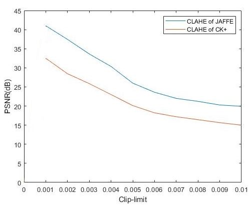
The PSNR
The PSNR results
PSNR results of CLAHE are
results of are shown in in Figure 7.7.
The of CLAHE
CLAHE are shownshown in Figure
Figure 7.Electronics 2019, 8, 324 10 of 16
Electronics 2019, 8, x FOR PEER REVIEW 10 of 16
Figure
Figure 7.
7. Peak
Peak signal
signal to
to noise
noise ratio
ratio (PSNR)
(PSNR) values
values of
of each
each variation.
It can be observed from
It from the
the figure
figurethat
thatthe
theCLAHE
CLAHEalgorithm
algorithmachieved
achievedthe
thehighest
highestPSNR
PSNR value at
value
CL = 0.001 in the JAFEE and CK+ databases.
at CL= 0.001 in the JAFEE and CK+ databases.
Secondly, we fixed the clip limit value
Secondly, value at
at 0.01
0.01 and
and varied
varied the
the block
block size
size from
from [2
[2 2]
2] to
to [128
[128 128],
128],
after
after which we calculated PSNR values of each variation (see Table 3).
3).
Table 3.
Table PSNR values
3. PSNR values of
of different
different block
block sizes.
sizes.
AveragePSNR
Average PSNR
Block Size
Block Size JAFFEDatabase
Database CK+ Database
JAFFE CK+ Database
2×2 17.43
17.43 12.13
12.13
2×2
4×4 18.22 13.89
84×× 84 18.22
19.92 13.89
15.00
168×× 16
8 16.61
19.92 11.94
15.00
32 × 32 15.53 10.75
16×× 64
64 16 16.61
14.49
11.94
9.99
32×× 128
128 32 15.53
11.21 10.75
7.20
64 × 64 14.49 9.99
It can be seen from the table
128 that the PSNR 11.21
× 128 achieved the highest7.20
value when the block size of [8 8]
for JAFEE and CK+ databases was used.
It can be seen from the table that the PSNR achieved the highest value when the block size of [8
8] forJAFFE
4.3. JAFEE and CK+ databases was used.
Database
The JAFFE
4.3. JAFFE database consists of 213 grayscale images of 10 Japanese female models; these images
Database
are almost frontal poses including 7 facial expression images; each image has a size of 256 × 256 [32].
The JAFFE
The following database of
illustration consists of 213isgrayscale
the database images8.of 10 Japanese female models; these
shown in Figure
imagesFirstly, we process the pictures from the JAFFE database asimages;
are almost frontal poses including 7 facial expression follows:each
the image
size of has a size
all the of 256
images was×
256 [32]. The
reduced to 64following
×64 pixels.illustration of the database is shown in Figure 8.
After that, contrast limited adaptive histogram equalization (CLAHE) was used for the
contrast enhancement.
Finally, we used 149 images for training (about 70% of the total) and 64 images for testing (about
30% of the total).
In Tables 4 and 5, N, A, D, F, H, Sa, and Su are used to represent seven basic expressions as neutral,
anger, disgust, fear, happiness, sadness, and surprise, respectively.8] for JAFEE and CK+ databases was used.
4.3. JAFFE Database
The JAFFE database consists of 213 grayscale images of 10 Japanese female models; these
images are
Electronics almost
2019, 8, 324 frontal poses including 7 facial expression images; each image has a size of11256 ×
of 16
Electronics 2019, 8, x FOR PEER REVIEW
256 [32]. The following illustration of the database is shown in Figure 8. 11 of 16
Figure 8. Partial image from the ORL database.
Firstly, we process the pictures from the JAFFE database as follows: the size of all the images
was reduced to 64×64 pixels.
After that, contrast limited adaptive histogram equalization (CLAHE) was used for the contrast
enhancement.
Finally, we used 149 images for training (about 70% of the total) and 64 images for testing
(about 30% of the total).
In Tables 4 and 5, N, A, D, F, H, Sa, and Su are used to represent seven basic expressions as
neutral, anger, disgust, fear, happiness, sadness, and surprise, respectively.
Table 4. The
Figure resultsimage
8. Partial obtained bythe
from theORL
JAFFE database.
database.
NThe results
Table 4. A obtained
D F by the
SaJAFFEHdatabase.
Su
N
N 98.5 A 0.2 0.8
D 0.2 F 0.0 0.1
Sa 0.0H Su
N 98.5
A 0.6 0.2 98.5 0.8
0.7 0.10.2 0.6 0.0
0.1 0.1
0.0 0.0
A 0.6 98.5 0.7 0.1 0.6 0.1 0.0
D D
0.0 0.0 0.9 0.9 99.2
99.2 0.00.0 0.1 0.1
0.1 0.0
0.1 0.0
F 0.2
F 0.2 0.5 0.5 0.5
0.5 97.5 0.5
97.5 0.5
0.1 0.1
0.7 0.7
S 0.7 0.2 0.0 0.8 98.9 0.0 0.3
H S
1.3 0.7 0.0 0.2 0.0
0.0 0.81.3 98.9 0.0
0.0 0.3
98.9 1.3
S 0.0
H 1.3 0.0 0.0 0.0
0.0 1.30.3 0.0 0.1
98.9 0.8
1.3 98.9
The proposed method S provided
0.0 high
0.0 recognition
0.0 0.3accuracy
0.1 of0.8
99.2%98.9
for disgust, 98.9% for surprise
happiness and sadness;
The proposed methodwhile anger, neutral,
provided and fear had
high recognition a high of
accuracy accuracy leveldisgust,
99.2% for but less98.9%
than the
for
previous
surprise facial expressions,
happiness with recognition
and sadness; accuracy
while anger, of 98.5%–97.5%
neutral, and fear hadrespectively. The JAFFE
a high accuracy level database
but less
achieved
than a recognition
the previous facialaccuracy of 98.63%.
expressions, with recognition accuracy of 98.5% – 97.5% respectively. The
JAFFE database achieved a recognition accuracy of 98.63%.
4.4. CK+ Database
4.4. CK+
TheDatabase
CK+ database consists of 593 images in total from 123 subjects that had a human facial
emotion
The based on the subject’s
CK+ database impression
consists of each
of 593 images in of the from
total seven123
basic emotions
subjects that[33].
had a human facial
emotion based on the subject’s impression of each of the seven basic emotions [33]. Euro–American,
The ages of participants are between 18 and 50, 69% of them are women, 81%
13% Afro-American, and 6% are
The ages of participants from other groups.
between Image
18 and 50, 69%sequences
of them areforwomen,
frontal 81%
views and 30-degree
Euro–American,
views were digitized into
13% Afro-American, and either
6% from × 490groups.
640 other or 640 ×Image
480 pixel arrays. for
sequences An frontal
illustration
viewsof the
anddatabase is
30-degree
shown in Figure 9.
views were digitized into either 640 × 490 or 640 × 480 pixel arrays. An illustration of the database is
shown in Figure 9.
Figure 9.
Figure 9. Partial
Partial image
image from
from the
the CK+
CK+ database.
database.
Firstly, the pictures from the CK+ database are processed as follows: the size of all the images
was reduced to 64 × 64 pixels.Electronics 2019, 8, 324 12 of 16
Firstly, the pictures from the CK+ database are processed as follows: the size of all the images was
reduced to 64 × 64 pixels.
After that, for contrast enhancement, contrast limited adaptive histogram equalization (CLAHE)
is used.
Finally, we used 415 images for training (about 70% of the total) and 178 images for testing (about
30% of the total).
Table 5. The results obtained by the CK+ database.
N A D F Sa H Su
N 100 0.2 0.8 0.2 0.0 0.1 0.0
A 0.6 95.0 0.6 0.1 0.6 0.2 0.0
D 0.0 1.0 98.5 0.0 0.1 0.1 0.0
F 0.2 0.5 0.5 93.7 0.5 0.2 0.7
S 0.7 0.2 0.0 0.8 93.1 0.0 0.3
H 1.2 0.0 0.0 1.2 0.0 99.4 1.1
S 0.0 0.0 0.0 0.3 0.1 1.0 99.7
The proposed method provided high recognition accuracy of 100% for neutral; 99.7% for surprised,
99.4% for happy, while angry disgust sad and fear had lower accuracy between 93.7% and 98.5%. The
CK+ database gives a recognition accuracy of 97.05%.
These results are satisfactory, but lower than those given using the JAFFE database; this is
because the images in the CK+ database were captured in a more difficult pose and under challenging
lighting conditions.
4.5. Results with and without Contrast Enhancement
In order to demonstrate the effect of CLAHE on the recognition rate, we made a comparison
between two methods; the first was used without the application of CLAHE.
The recognition rate results without the application of CLAHE enhancement algorithm for the
JAFEE and CK+ database are shown in Table 6.
Table 6. Results without the application of CLAHE. RR—recognition rate.
Expression RR(%) for JAFEE RR(%) for CK+
Neutral 96.60 98.3
Anger 97.10 93.7
Disgust 97.30 96.5
Fear 96.17 92.4
Happy 96.63 90.8
Sad 96.90 97.3
Surprise 97.17 98.1
The second method with the application of CLAHE provided the results shown in Table 7.
Table 7. Results with the application of CLAHE.
Expression RR(%) for JAFEE RR(%) for CK+
Neutral 98.5 100
Anger 98.5 95.0
Disgust 99.2 98.5
Fear 97.5 93.7
Happiness 98.9 93.1
Sadness 98.9 99.4
Surprise 98.9 99.7Electronics 2019, 8, 324 13 of 16
The comparison of the two methods with CLAHE and without CLAHE will show an improvement
in the results, the recognition rate of the JAFFE database is improved by 1.9% for neutral, 1.4% for
anger, 1.9% for disgust, 1.33% for fear, 2.27% for happiness, 2% for sadness, and 1.73% for surprise.
For the CK+ database, the recognition rate has increased by 1.7% for neutral, 1.3% for anger, 2%
for disgust, 1.3% for fear, 2.3% for happiness, 2.1% for sadness, and 1.6% for surprise.
4.6. Comparison with Other Methods
In order to prove the effectiveness of our approach, the average recognition accuracy is compared
with other approaches for FER.
Tables 8 and 9 show the comparison of the recognition accuracy obtained with our approach and
with other approaches for the JAFFE and CK+ databases.
Table 8. The comparison between different approaches and our approach for the JAFFE face database.
CNN— convolutional neural network.
Approach Recognition Rate %
SVM [34] 95.60
Gabor [35] 93.30
2-Channel CNN [12] 94.40
Deep CNN [14] 97.71
Normalization+ DL [36] 88.73
Viola-Jones+ CNN 95.30
Proposed Method 98.63
Table 9. The comparison between different approaches and our approach for the CK+ face
database.CNN— convolutional neural network.
Approach Recognition Rate %
SVM [37] 95.10
Gabor [35] 90.62
3D-CNN [38] 95.00
Deep CNN [14] 95.72
Normalization+ DL [36] 93.68
Viola-Jones+ CNN 95.10
Proposed Method 97.05
From the data in Tables 8 and 9, it is clear that our approach has achieved the highest recognition
rate compared with CNN and the other approaches.
4.7. Training Time
In this section, we compared the training times of the CNN algorithm and the proposed algorithm
in both databases. The comparison results are shown in Table 10.
Table 10. The training times comparison.
Algorithm JAFFE CK+
CNN algorithm 20.3 s 33.3 s
Proposed algorithm 15.7 s 26 s
It can be seen from Table 10 above that the training time of the proposed algorithm is much
shorter than that of the CNN algorithm; this means that our approach has a higher training speed
and efficiency.
In short, the proposed algorithm greatly outperforms the traditional algorithm in terms of speed,
recognition accuracy, and efficiency.Electronics 2019, 8, 324 14 of 16
5. Conclusions
This work presents a method of facial expressions recognition (FER) based on the Viola-Jones
face detection algorithm, and facial image enhancement algorithms to improve image contrast. A
comparative study of all these techniques has been presented. Through the results achieved after
calculation of PSNR and AMBE parameters, we found that CLAHE outperforms all other techniques.
Indeed, CLAHE clearly improves the contrast and brightness of the image more than the other
enhancement techniques.
Then discrete wavelet transforms (DWT) and deep CNN are presented in this paper. Features
extraction results of the face using DWT are the input to CNN network training, and the trained
network is used for facial expressions recognition.
This network consists of three ConvL, two pooling layers, a fully-connected layer, and one softmax
regression layer to classify and complete facial expressions recognition.
The results achieved on the JAFFEE and CK+ database confirm the effectiveness and robustness of
our method. In experiments on the testing set of the JAFEE database and CK+ database, the expression
recognition rate reaches up to 98.63% and 97.05%, respectively.
Author Contributions: Conceptualization, R.I.B. and K.M.; methodology, R.I.B.; software, R.I.B.; validation,
R.I.B., K.M. and M.B.; formal analysis, M.B.; investigation, A.T.-A.; resources, R.I.B.; data curation, R.I.B.;
writing—original draft preparation, R.I.B.; writing—review and editing, R.I.B. and A.T.-A.; visualization, K.M.;
supervision, M.B.; project administration, M.B. and A.T.-A.
Funding: This research received no external funding.
Acknowledgments: This work is supported by a research project about design and implementation of a
surveillance system based on biometric systems for the detection and recognition of individuals and abnormal
behaviors (N◦ A25N01UN080120180002).
Conflicts of Interest: The authors declare no conflict of interest.
Abbreviations
AHE Adaptive Histogram Equalization
AMBE Absolute Mean Brightness Error
CDF Cumulative Distribution Function
ConvL Convolutional Layers
CLAHE Contrast Limited Adaptive Histogram Equalization
CNN Convolutional Neural Network
DWT Discrete Wavelet Transform
FER Facial Expressions Recognition
HE Histogram Equalization
LBP Local Binary Patterns
PDF Probability Density Function
PSNR Peak Signal to Noise Ratio
RELU Rectified Linear Unit
WMDNN Weighted Mixture Deep Neural Network
References
1. Yin, Y.; Li, Y.; Li, J. Face Festure Extraction Based on Principle Discriminant Information Analysis. In
Proceedings of the IEEE International Conference on Automation and Logistics, Jinan, China, 18–21 August
2007; pp. 1580–1584.
2. Pantic, M.; Rothkrantz, L.J. Automatic analysis of facial expressions: The state of the art. IEEE Trans. Pattern
Anal. Mach. Intell. 2000, 22, 1424–1445. [CrossRef]
3. Wiskott, L.; Fellous, J.M.; Kuiger, N.; Malsburg, C.V. Face Recognition by Elastic Bunch Graph Matching.
IEEE Trans. Pattern Anal. Mach. Intell. 1997, 19, 775–779. [CrossRef]
4. Bartlett, M.S.; Movellan, J.R.; Sejnowski, S. Face Recognition by Independent Component Analysis. IEEE
Trans. Neural Netw. 2002, 13, 1450–1464. [CrossRef] [PubMed]Electronics 2019, 8, 324 15 of 16
5. Belhumeur, P.N.; Hespanha, J.P.; Kriegman, D.J. Eigenfaces vs. Fisherfaces. IEEE Trans. Pattern Anal. Mach.
Intell. 1997, 19, 711–720. [CrossRef]
6. Turk, M.; Pentland, A. Eigenfaces for Recognition. Cogn. Neurosci. 1991, 3, 71–86. [CrossRef] [PubMed]
7. Zhang, T.; Zheng, W.; Cui, Z.; Zong, Y.; Yan, J.; Yan, K. A deep neural network driven feature learning
method for multi-view facial expression recognition. IEEE Trans. Multimed. 2016, 18, 2528–2536. [CrossRef]
8. Kim, D.J.; Chung, K.W.; Hong, K.S. Person authentication using face, teeth, and voice modalities for mobile
device security. IEEE Trans. Consum. Electron. 2010, 56, 2678–2685. [CrossRef]
9. Wang, M.; Jiang, H.; Li, Y. Face Recognition based on DWT/DCT and SVM. In Proceedings of the
International Conference on Computer Application and System Modeling (ICCASM 20ID), Taiyuan, China,
22–24 October 2010; pp. 507–510.
10. Liu, M.; Li, S.; Shan, S.; Wang, R.; Chen, X. Deeply learning deformable facial action parts model for dynamic
expression analysis. In Computer Vision–ACCV 2014; Springer: Cham, Switzerland, 2014; pp. 143–157.
[CrossRef]
11. Burkert, P.; Trier, F.; Afzal, M.Z.; Dengel, A.; Liwicki, M. DeXpression: Deep Convolutional Neural Network
for Expression Recognition. arXiv, 2015; arXiv:1509.05371.
12. Hamester, D.; Barros, P.; Wermter, S. Face Expression Recognition with a 2-Channel Convolutional Neural
Network. In Proceedings of the International Joint Conference on Neural Networks (IJCNN), Killarney,
Ireland, 12–17 July 2015.
13. Cui, R.; Liu, M.; Liu, M. Facial Expression Recognition Based on Ensemble of Multiple CNNs. In Proceedings
of the Biometric Recognition: 11th Chinese Conference, CCBR 2016, LNCS 9967, Chengdu, China, 14–16
October 2016; pp. 511–578.
14. Nwosu, L.; Wang, H.; Lu, J.; Unwal, I.; Yang, X.; Zhang, T. Deep Convolutional Neural Network for Facial
Expression Recognition using Facial Parts. In Proceedings of the IEEE 15th International Conference on
Dependable, Autonomic and Secure Computing, Orlando, FL, USA, 6–10 November 2017; pp. 1318–1321.
15. Yang, B.; Cao, J.; Ni, R.; Zhang, Y. Facial Expression Recognition Using Weighted Mixture Deep Neural
Network Based on Double-Channel Facial Images. IEEE Access 2018, 6, 4630–4640. [CrossRef]
16. Viola, P.; Jones, M. Robust real-time object detection. In Proceedings of the Second International Work Shop
on Statistical and Computational Theories of Vision, Vancouver, CA, Canada, 13 July 2001.
17. Vikram, K.; Padmavathi, S. Facial parts detection using Viola Jones Algorithm. In Proceedings of the 2017
4th International Conference on Advanced Computing and Communication Systems (ICACCS), Coimbatore,
India, 6–7 January 2017.
18. Lee, P.-H.; Wu, S.-W.; Hung, Y.-P. Illumination compensation using oriented local histogram equalization
and its application to face recognition. IEEE Trans. Image Process. 2012, 21, 4280–4289. [CrossRef] [PubMed]
19. Abdullah-Al-Wadud, M.; Kabir, M.H.; Dewan, M.A.A.; Chae, O. A Dynamic Histogram Equalization for
Image Contrast Enhancement. IEEE Trans. Consum. Electron. 2007, 53, 593–600. [CrossRef]
20. Huang, L.; Zhao, W.; Wang, J.; Sun, Z. Combination of contrast limited adaptive histogram equalization and
discrete wavelet transform for image enhancement. IET Image Process. 2015, 9, 908–915.
21. Dharani, P.; Vibhute, A.S. Face Recognition Using Wavelet Neural Network. Int. J. Adv. Res. Comput. Sci.
Softw. Eng. 2017, 7. [CrossRef]
22. Benzaoui, A.; Boukrouche, A.; Doghmane, H.; Bourouba, H. Face recognition using 1dlbp, dwt and svm. In
Proceedings of the 2015 3rd International Conference on Control, Engineering & Information Technology
(CEIT), Tlemcen, Algeria, 25–27 May 2015; pp. 1–6.
23. Dawoud, N.N.; Samir, B.B. Best Wavelet Function for Face Recognition Using Multi-Level Decomposition.
In Proceedings of the IEEE International Conference on Research and Innovation in Information Systems,
Nanjing, China, 24–25 September 2011.
24. Arel, D.; Rose, D.C.; Karnowski, T.P. Deep machine learning—A new frontier in artificial intelligence research
[research frontier]. IEEE Comput. Intell. Mag. 2010, 5, 13–18. [CrossRef]
25. Coúkun, M.; Uçar, A.; Yildirim, Ö.; Demir, Y. Face Recognition Based on Convolutional Neural Network. In
Proceedings of the International Conference on Modern Electrical and Energy Systems (MEES), Kremenchuk,
Ukraine, 15–17 November 2017; pp. 376–379.
26. Wang, M.; Wang, Z.; Li, J. Deep Convolutional Neural Network Applies to Face Recognition in Small
and Medium Databases. In Proceedings of the 4th International Conference on Systems and Informatics,
Hangzhou, China, 11–13 November 2017; pp. 1368–1378.Electronics 2019, 8, 324 16 of 16
27. Yan, K.; Huang, S.; Song, Y.; Liu, W.; Fan, N. Face Recognition Based on Convolution Neural Network. In
Proceedings of the 36th Chinese Control Conference, Dalian, China, 26–28 July 2017; pp. 4077–4081.
28. Zhou, N.; Wang, L.P. Class-dependent feature selection for face recognition. In Proceedings of the 15th
International Conference (ICONIP 2008), Auckland, New Zealand, 25–28 November 2008; pp. 551–558.
29. El Shafey, L.; Mccool, C.; Wallace, R.; Marcel, S. A Scalable Formulation of Probabilistic Linear Discriminant
Analysis: Applied to Face Recognition. IEEE Trans. Pattern Anal. Mach. Intell. 2013, 35, 1788–1794. [CrossRef]
30. Sahu, S. Comparative Analysis of Image Enhancement Techniques for Ultrasound Liver Image. Int. J. Electr.
Comput. Eng. 2012, 2, 792–797. [CrossRef]
31. Kim, M.; Chung, M.G. Recursively Separated and Weighted Histogram Equalization for Brightness
Preservation and Contrast Enhancement. IEEE Trans. Consum. Electron. 2008, 54, 1389–1397. [CrossRef]
32. Lyons, M.J.; Akamatsu, S.; Kamachi, M.; Gyoba, J. Coding Facial Expressions with Gabor Wavelets. In
Proceedings of the third IEEE International Conference on Automatic Face and Gesture Recognition, Nara,
Japan, 14–16 April 1998; pp. 200–205.
33. Kanade, T.; Cohn, J.F.; Tian, Y. Comprehensive database for facial expression analysis. In Proceedings of
the Fourth IEEE International Conference on Automatic Face and Gesture Recognition (FG’00), Grenoble,
France, 26–30 March 2000; pp. 46–53.
34. Santiago, H.C.; Ren, T.; Cavalcanti, G.D.C. Facial expression Recognition based on Motion Estimation. In
Proceedings of the 2016 International Joint Conference Neural Networks (IJCNN), Electronic Vancouver, BC,
Canada, 24–29 July 2016.
35. Al-Sumaidaee, S.A.M. Facial Expression Recognition Using Local Gabor Gradient Code-Horizontal Diagonal
Dedscriptor. In Proceedings of the 2nd IET International Conference on Intelligent Signal Processing 2015
(ISP), London, UK, 1–2 December 2015.
36. Lopes, A.T.; de Aguiar, E.; de Souza, A.F.; Oliveira-Santos, T. Facial expression recognition with convolutional
neural networks: Coping with few data and the training sample order. Pattern Recognit. 2017, 61, 610–628.
[CrossRef]
37. Shan, C.; Gong, S.; McOwan, P.W. Facial expression recognition based on local binary patterns: A
comprehensive study. Image Vis. Comput. 2009, 27, 803–816. [CrossRef]
38. Byeon, Y.-H.; Kwak, K.-C. Facial expression recognition using 3d convolutional neural network. Int. J. Adv.
Comput. Sci. Appl. 2014, 5. [CrossRef]
© 2019 by the authors. Licensee MDPI, Basel, Switzerland. This article is an open access
article distributed under the terms and conditions of the Creative Commons Attribution
(CC BY) license (http://creativecommons.org/licenses/by/4.0/).You can also read