Firearms Law and Fatal Police Shootings: A Panel Data Analysis
←
→
Page content transcription
If your browser does not render page correctly, please read the page content below
Firearms Law and Fatal Police Shootings:
                                                                           A Panel Data Analysis
arXiv:2101.03131v1 [econ.GN] 8 Jan 2021

                                                                     Marco Rogna∗1 and Bich Diep Nguyen2
                                                             1
                                                                 Department of Economics, Bochum University of Applied Sciences
                                                 2
                                                     Faculty of Political Theory - Civic Education, Hanoi National University of Education

                                            ∗
                                                Correspondence: Marco Rogna, Department of Economics, Bochum University of Applied Sci-
                                          ences, Am Hochschulcampus 1, 44801 Bochum, Germany. Email: marco.rogna@hs-bochum.de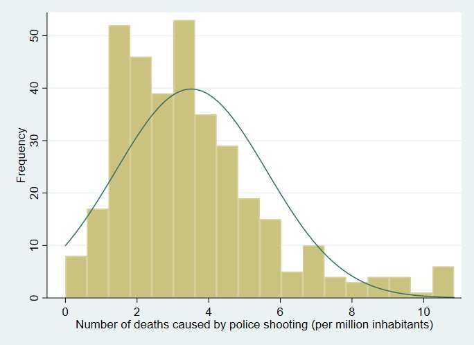
Abstract

   Among industrialized countries, U.S. holds two somehow inglorious records:
the highest rate of fatal police shootings and the highest rate of deaths related
to firearms. The latter has been associated with strong diffusion of firearms
ownership largely due to loose legislation in several member states. The present
paper investigates the relation between firearms legislation\diffusion and the
number of fatal police shooting episodes using a seven-year panel dataset. While
our results confirm the negative impact of stricter firearms regulations found
in previous cross-sectional studies, we find that the diffusion of guns ownership
has no statistically significant effect. Furthermore, regulations pertaining to the
sphere of gun owner accountability seem to be the most effective in reducing
fatal police shootings.

Keywords: Police shootings; Firearms law; Guns diffusion; Panel data.
J.E.L. I12; I18.
Introduction
The Unites States (U.S.) is one of the countries with the highest firearms–related
death rate, exceptionally high compared to other industrialized countries (Pallin et al.,
2019). Furthermore, it is the country with the highest firearms possession rate by
citizens, thanks to loose legislation in several of its member states (Hemenway, 2017).
The relation between firearms–related death rate and firearms possession rate has
been largely investigated and a causal relation going from the latter to the for-
mer seems very plausible, e.g. Krug et al. (1998); Bangalore and Messerli (2013)
and Siegel et al. (2013). If this fact has prompted part of the public opinion to ask
for stricter guns laws, the constitutional right to posses and bear firearms has been
strenuously defended by the opposite faction, rendering this one of the most popular
and controversial topic in the country.
   Almost every aspect of the relation between firearms legislation and gun vio-
lence has been extensively researched. Besides the mentioned studies that have tried
to establish a causal link between firearms–related death rate and firearms posses-
sion rate (Krug et al., 1998; Bangalore and Messerli, 2013; Siegel et al., 2013), others
have investigated the effect of firearms legislation\possession rate on suicide rates
(Kellermann et al., 1992; Anestis and Houtsma, 2018), on pediatric firearms–related
mortality Goyal et al. (2019), on homicides rate (Duggan, 2001; Kovandzic et al.,
2013; Siegel et al., 2013, 2014), and on the death rate of police officers on duty (Lester,
1987; Mustard, 2001; Swedler et al., 2015).
   With approximately 1000 deaths per year, United States (U.S.) holds another
inglorious record among industrialized countries: the highest rate of homicides com-
mitted by police forces (Hemenway et al., 2019). This raises the question of whether
the high rate of police fatal shootings results from relaxed firearms legislation\high
possession rate. From a speculative point of view, one can argue that the diffusion of

                                            1
firearms increases the probability of police officers to face armed people while on duty,
thus increasing the probability of being involved in potentially dangerous situations
that require the use of guns from their part. Furthermore, the increased probabil-
ity to face dangerous situations is a factor of stress that may lead law enforcement
officers to overreact or, more generally, to commit mistakes. A positive relation be-
tween firearms diffusion and deadly assaults to police officers (Swedler et al., 2015)
corroborates the theory of an increase danger to officers for higher levels of firearms
ownership.
Thanks to the availability of independent datasets that remedy the underreporting
of police fatal use of force in official statistics (Conner et al., 2019), this topic has re-
cently been investigated. Hemenway et al. (2019) find a positive association between
firearms prevalence and fatal police shooting rates. Kivisto et al. (2017) report that
U.S. states with stricter firearms legislation have lower incidence rates of fatal po-
lice shootings. Both studies are, however, cross-sectional and thus, despite the use of
several controls common in the dedicated literature, may suffer from the omitted vari-
able problem. Kivisto et al. (2017), for example, mention, among the limitations of
their paper, exactly this problem, stating that “it is possible that states with stricter
gun legislation also have better training for police officers and more stringent hiring
practices, or that states that are already safe are more likely to implement stricter
gun laws”.
The novelty of the present study is to use a panel dataset to investigate the relation
between firearms legislation\possession rate and fatal police shootings. This allows
to control for unobserved fixed characteristics at state level that may have biased
previous analysis, providing, therefore, more robust results.
21 Literature Review
As discussed before, firearms legislation and ownership is a strongly investigated topic,
particularly in the United States. A number of studies document negative impacts
of firearms legislation and prevalence, such as increased suicide and homicide rate,
although evidence is not unambiguous. From an extensive literature review, Kleck
(2015) concludes that guns diffusion is a positive determinant of crime rate, but this
relation looses statistical significance in the most methodologically rigorous papers.
Branas et al. (2009) find that possessing a gun increases the probability of being shot
during an assault, thus dismantling the opinion of weapons having a protective role.
On the other side, Kleck and Patterson (1993), by comparing 170 U.S. cities, find
scarce evidence that guns restrictions have some positive role in reducing the rate of
violence. Similarly, Altheimer (2008) evidences that gun availability has no effect in
determining the number of total individual assaults and robbery, but only increases
the number of the ones committed with a fire–weapon.
Regarding one of the most serious violent crimes, homicide, the results are mixed.
Duggan (2001), Siegel et al. (2013) and Siegel et al. (2014) find a significant and
positive relation between guns diffusion and the number of homicides. However,
this view is strongly opposed by Kovandzic et al. (2013), which, on the contrary,
document a negative relation. They cite a potential deterrent effect of guns as an
explanation for their results. A similar debate has surrounded the permission of
carrying concealed weapons, with Lott and Mustard (1997) showing a positive role of
such law in reducing violent crimes whereas Dezhbakhsh and Rubin (1998) rejecting
this finding and claiming the opposite. Findings regarding firearms diffusion and
legislation are therefore very discordant even when considering aspects such as crime
and homicide rate that are among the most studied.
Shifting the attention on police forces, there is a paucity of research regarding the
3association between firearms diffusion and legislation and the number of killings of,
and by, police officers. When considering the former, the killing of law enforcement
officers, we have again contrasting findings. Lester (1987) and Swedler et al. (2015)
find that increasing levels of households gun ownership are a clear factor of risk for
police officers, whereas Mustard (2001), limiting the attention to the possibility of
carrying concealed weapons, puts in evidence a potential protective role of this law.
Kivisto et al. (2017) and Hemenway et al. (2019) investigate the relation between
firearms and killings committed by police officers. The two studies both rely on in-
dependent and open source databases to retrieve the number of fatal police shootings:
Kivisto et al. (2017) on The Counted, maintained by The Guardian, and Hemenway et al.
(2019) on Fatal Force, created by The Washington Post. Furthermore, they both rely
on a cross sectional analysis using the fraction of suicides with a fire–weapon on the
total number of suicides as a proxy for guns diffusion, as previously done in other
papers, e.g. Kleck (2004) and Azrael et al. (2004). Compared to Hemenway et al.
(2019), whose focus is exclusively on guns diffusion as a cause of fatal police shootings,
Kivisto et al. (2017) further consider firearms legislation, using the Brady Campaign
scorecards as an indicator of law strength. In both papers, firearms ownership is
found to positively affect the number of fatal police shootings. Even after control-
ling for firearms prevalence, firearms regulations on gun trafficking and on child and
consumer safety significantly reduces fatal police shootings (Kivisto et al., 2017).
Given the contrasting evidence emerged in other topics related to firearms diffusion
and legislation and since both the last mentioned papers rely on a cross sectional
analysis that may be plagued by the omitted variable bias, the extension to a panel
data setting seems a necessary further step. This may help to strengthen the findings
reached so far or to contest their validity as the result of a biased analysis.
42 Data and Methods
Following Kivisto et al. (2017) and Hemenway et al. (2019), our units of observa-
tion are the 50 U.S. states, with District of Columbia having being excluded for
lack of data in several covariates. The covered time period is from January 1,
2012, to December 31, 2018, and all variables are expressed as yearly values, form-
ing a dataset with seven time periods. Different databases have been consulted
and merged in order to have all the variables of interest and the necessary con-
trols: Fatal Encounters, Giffords scorecards, the U.S. Census Bureau data portal, the
Federal Bureau of Investigation’s (FBI’s) Crime Data Explorer and the Centers for
Disease Control and Prevention’s (CDC’s) Web-based Injury Statistics Query and Reporting System
(WISQARS). Following is a description of all variables.
2.1 Description of Variables
Our dependent variable, the number of deaths caused by police shooting per million
inhabitants (Pol Shoot), is retrieved from the Fatal Encounters database. We choose
an independent database to alleviate the likely problem of underreporting of such
episodes in the FBI’s official statistics (Williams et al., 2019). Compared to other
open source repositories, e.g. The Counted, Fatal Force, Mapping Police Violence
and Gun Violence Archive, the Fatal Encounters database covers the longest time
span – from 2000 to present. Specific cases of police shooting can be retrieved by
selecting the category “Deadly use of force” and the subcategory “Gunshot”.
Our independent variable of interest is the strength of firearms regulations at state
level (Giff Score). In order to obtain a synthetic measure of the strength of a state
legislation, we rely on the Giffords scorecards, available for the period 2010-2018, with
the exclusion of the year 2011, hence the need to drop the year 2010. The overall
score is an aggregation of seven component scores, namely: background checks and
5access to firearms (BCAF ), other regulations of sales and transfers (ORST ), classes of
weapons and magazines\ammunitions (CWAM ), consumers and child safety (CCS ),
gun owner accountability (GOA), firearms in public places (FPP) and a residual
class (OTH ). Disaggregation of the overall score allows us to test the role of each
component in explaining fatal police shootings, following Kivisto et al. (2017). This
is helpful in identifying the areas where intervention should be prioritized to reduce
police shooting episodes. Since the scoring system has been slightly modified several
times during the study period, we have implemented a harmonization procedure,
retaining only the sub-indicators that remained unaltered over time. Kivisto et al.
(2017), using data from the same source, eliminate the weighting system in favor of
a “1 law = 1 point” scale. They argue that a weighting system necessarily entails a
degree of arbitrariness. However, we think that the equal weighting implied by the
“1 law = 1 point” scale is analogously arbitrary. We, therefore, prefer to rely on
the weights assigned by professional lawyers, thus leaving the Giffords scorecard scale
unaltered.
Stricter legislation on firearms may reduce the quantity of fire–weapons owned by
citizens, but may also promote safer use, e.g. by denying dangerous subjects access
to guns or by increasing the safety of circulating weapons. Besides examining if laws
to promote safe gun use are effective in reducing fatal police shootings, we can test
if the effect of firearms legislations operate via the former channel by looking at the
relation between fatal police shootings and gun diffusion. Lacking state–level data on
gun ownership for our study period, we rely on a commonly adopted proxy (Suicide)
– the percentage of suicides committed with a fire–weapon over the total of suicides
(Kleck, 2004; Azrael et al., 2004; Kivisto et al., 2017; Hemenway et al., 2019). These
data are retrieved from the Web-based Injury Statistics Query and Reporting System
(WISQARS).
6Table 1: Descriptive Statistics
Variable N. Obs. Mean Std. Dev. Min. Max.
Pol Shoot 350 3.51 2.11 0 10.85
Giff Score 350 31.98 24.42 4 105.50
Crime 350 3627.32 1388.63 1026.24 8849.56
Suicide 350 51.54 12.35 13.20 74.30
PC Income 350 29712.58 4828.93 20119 52500.00
Urban 350 73.59 14.44 38.70 95
Poverty 350 9.99 2.80 4 19.20
White 350 76.95 12.67 24.30 95.10
Low Edu 350 11.19 2.97 6.10 18.60
Unemp. 350 3.96 1.18 1.80 7.90
Young 350 23.15 1.31 19.80 27.50
Giff Score disentangled
BCAF 350 7.19 5.51 0 22
ORST 350 4.12 5.89 0 24
CWAM 350 1.82 3.86 0 14
CCS 350 2.25 2.02 0 9
GOA 350 2.76 5.00 0 17.50
FPP 350 9.16 4.36 0 19
OTH 350 4.67 2.18 0 10
Regarding control variables, we retrieved data on the number of violent crimes
(per million inhabitants, Crime) from the FBI’s Crime Data Explorer, where a crime
is defined as any of the four offenses – murder and non-negligent manslaughter, rape,
robbery, and aggravated assault. All the other controls are retrieved from the U.S.
Census Bureau. Note that all values are projections on the 2010 census data. These
controls include per–capita income in 2010 inflation–adjusted dollars (PC Income)
and the percentage of people living in urban areas (Urban). It must be noted that,
7for this last variable, only figures for the year 2010 were available, thus it is treated
as a time–invariant covariate. Other socio–economic characteristics, such as poverty
rate (Poverty), unemployment rate (Unemp.), and the percentage of adults with
an education lower than high school diploma (Low Edu), are also included. The
percentage of young population, aged 18–34, (Young) and the percentage of white
Caucasians (White) over the whole population are controlled for in the analysis. The
last variable is added since several studies find a racial bias in police shootings (Ross,
2015; Nix et al., 2017; Mesic et al., 2018). Table 1 reports some key statistics of all
the mentioned variables.
2.2 Statistical Analysis
The statistical analysis is divided into two main parts. In the first part, we focus on the
role of the legislative strength as a whole, thus considering the overall score provided
by Giffords for each U.S. state. In the second part, we analyze the component Giffords
scores separately. This analysis should provide more specific policy indications with
regard to the legislative field where intervention may be more productive in reducing
fatal police shootings.
The effects of any changer in legislation may take time to be observed. In all
our analysis, therefore, both the overall and the component Giffords scores enter
in their first lags. The inclusion of lags more distant in time (two or three years) is
precluded by the limited number of time periods at our disposal. We have actually run
regressions with the contemporaneous level of the Giffords scores, but none of them
has resulted in significant coefficients (results are available from the authors upon
request). The possibility to include both the lag and the current level is prevented
by their high correlation (ρ = 0.99) that most likely causes a problem of collinearity.
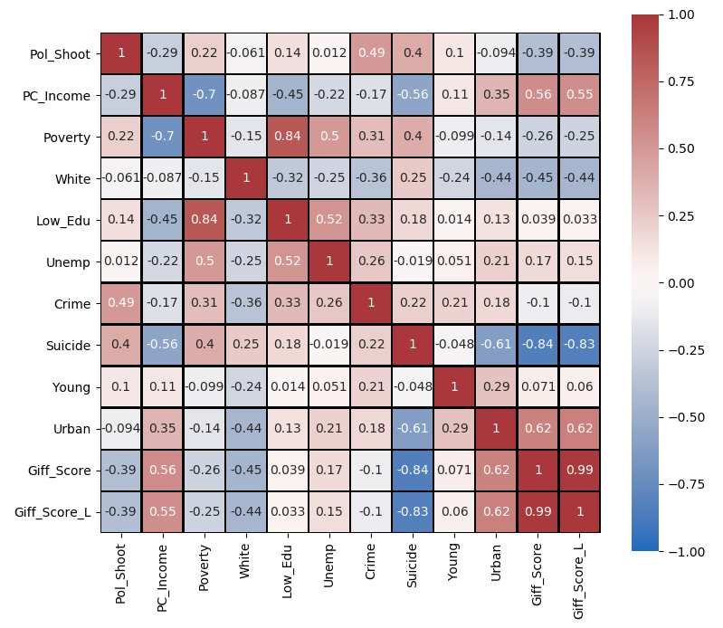
Figure 1 shows the Spearman’s rank correlation coefficients of all variables, except
8the component Giffords score. Note Giff Score L denotes the lagged Giffords score.
From Figure 1 it is possible to observe that several covariates have a relatively low
correlation coefficient. The exceptions are the violent crime rate (ρ = 0.49) and the
per–capita income (ρ = −0.29).
Figure 1: Correlation Matrix
Despite the low correlation of these covariates with the dependent variable, our
full specifications (specifications (1) and (2) in Table 2) include all of them. Their
9coefficients are not significant in these models. Failing to reject the null hypothesis
that the joint significance of the socio–economic covariates (Poverty, White, Low Edu,
Unemp. and Young) is equal to zero (p–value = 0.6098 for model (1) and p–value
= 0.8595 for model (2)), we omit these variables in any subsequent analysis. Despite
its lack of significance, Urban is kept in all models because of its high correlation
with the lagged Giffords score (ρ = 0.62) and because it is a significant control in
previous studies (Hemenway et al., 2019). Models (3) and (4) in Table 2 report the
results with the parsimonious set of explanatory variables. From Table A1 in the
Appendix, it is possible to observe non significant p–values for the RESET and for
the Mundlak test. Compared to models (1) and (2), the coefficients of models (3)
and (4) are negligibly different.
A conditional fixed effect (FE) and a random effect (RE) Poisson regressions
(models (1) and (2) in Table 2) are our main models of interest. The functional form
specification is checked through a RESET test, by adding the squared residuals of
the Poisson regressions (FE and RE) and checking their significance (Ramsey, 1974).
Results are reported in Table A1 in the Appendix together with the coefficients of the
year dummies (year 2013 as base) included in all models. The p–value of the squared
residuals is far above the 10% significance level, thus dismissing possible concerns
about misspecification. The choice to report both the FE and RE estimates is due to
the fact that the Mundlak test – also reported in Table A1 – has a significance level
very close to the 5% level (Mundlak, 1978). Although this test, chosen compared
to the more common Hausman test given the presence of year dummies and a time
invariant covariate (Urban), suggests the use of the random effect model, the close-
ness of the p–value to the threshold level and the concerns about the distributional
assumptions of the Poisson RE model lead us to report the fixed effect estimates as
well. However, it can be observed that the estimated coefficients are very similar in
both specifications.
10Table 2: Regressions Results: Total Giffords Score (Lagged)
(1) (2) (3) (4)
Poisson FE Poisson RE Poisson FE Poisson RE
Pol Shoot Pol Shoot Pol Shoot Pol Shoot
0.990* 0.992+ 0.990* 0.993+
Giff Score L
(-2.05) (-1.65) (-2.10) (-1.82)
1.000 1.000*** 1.000 1.000***
Crime
(1.61) (4.04) (1.46) (4.69)
0.993 1.007 0.993 1.008
Suicide
(-0.77) (1.03) (-0.76) (1.21)
1.000* 1.000* 1.000 1.000+
PC Income
(-2.15) (-2.05) (-1.49) (-1.94)
1.004 1.005
Urban
(0.90) (1.32)
0.958 0.965
Poverty
(-1.51) (-1.04)
0.958 0.996
White
(-1.21) (-0.66)
1.025 1.012
Low Edu
(0.90) (0.38)
1.064 1.032
Unemp.
(1.20) (0.80)
0.946 1.008
Young
(-1.01) (0.23)
t-statistics in parentheses. P-value: + p2000). The results of the linear models are shown in Table 3. Although the transfor-
mation of the dependent variable prevents the computation of meaningful marginal
effects, the sign and significance of the coefficients serve to confirm the results of, or
to signal a possible problem in, the Poisson regressions. The distribution of the de-
pendent variable before and after the Yeo–Johnson transformation is shown in Figure
A1 in the Appendix.
For our second purpose, we regress the rate of fatal police shootings on the com-
ponent Giffords scores rather than the overall score. Here we present only the parsi-
monious models. Four models have been run, two Poisson – FE and RE – and two
analogous linear regressions. Results are reported in Table 4, models (5), (6), (7) and
(8), and auxiliary information can be found in Table A1 in the Appendix. From this
last table, it is possible to see that the p–values of the RESET and of the Mundlak
test are all above conventional significance levels. As for the previous models, the
difference in the significance of the coefficients of the Poisson and of the linear regres-
sions are very modest, so as the difference in the coefficients between the FE and RE
models.
12Table 3: Regressions Results: Linear Models
(1b) (2b) (3b) (4b)
Linear FE Linear RE Linear FE Linear RE
Pol Shoot Pol Shoot Pol Shoot Pol Shoot
-0.00879* -0.00924** -0.00925* -0.00803*
Giff Score L
(-2.32) (-2.86) (-2.34) (-2.52)
1.47-E004+ 1.36-E004*** 1.60-E004+ 149-E004***
Crime
(1.76) (3.75) (1.95) (4.43)
-0.00515 0.00193 -0.00562 0.00237
Suicide
(-0.55) (0.36) (-0.59) (0.45)
-1.83-E005* -1.95-E005* -1.44-E005+ -155-E005*
PC Income
(-2.07) (-2.22) (-1.75) (-2.12)
0.00255 0.00357
Urban
(0.66) (0.92)
-0.0248 -0.0259
Poverty
(-0.80) (-0.87)
-0.0159 -0.00411
White
(-0.41) (-1.03)
0.0142 0.0124
Low Edu
(0.51) (0.52)
0.0393 0.0327
Unemp.
(0.64) (0.69)
-0.0476 -0.0138
Young
(-0.92) (-0.47)
4.304 2.195* 1.938** 1.291*
Const.
(1.34) (2.06) (2.83) (2.42)
0.0538 0.0639 0.0313 0.0418
2014
(0.76) (0.92) (0.46) (0.60)
0.0661 0.0829 0.0359 0.0522
2015
(0.84) (1.15) (0.52) (0.76)
0.137 0.151+ 0.113* 0.120*
2016
(1.55) (1.95) (2.24) (2.48)
0.163 0.189+ 0.129+ 0.146*
2017
(1.42) (1.75) (1.99) (2.31)
0.255* 0.282* 0.220** 0.236***
2018
(2.11) (2.40) (3.10) (3.36)
t-statistics in parentheses. P-value: + pTable 4: Regressions Results: Giffords Score Disentangled (Lagged)
(5) (6) (7) (8)
Poisson FE Poisson RE Linear FE Linear RE
Pol Shoot Pol Shoot Pol Shoot Pol Shoot
1.001 1.000 0.00131 -6.63-E004
BCAF L
(0.15) (0.03) (0.22) (-0.12)
1.032 1.008 0.0231 0.0110
ORST L
(1.44) (0.47) (1.17) (0.93)
0.981 1.014 -0.0168 0.00372
CWAM L
(-0.93) (0.44) (-1.01) (0.22)
0.926 0.958 -0.0732 -0.0409
CCS L
(-1.09) (-1.24) (-1.19) (-1.47)
0.963* 0.962* -0.0351* -0.0352**
GOA L
(-2.57) (-2.32) (-2.58) (-2.93)
0.984 0.983 -0.0191 -0.0193
FPP L
(-1.25) (-1.38) (-1.54) (-1.63)
1.000 1.000*** 1.58-E004+ 1.57-E004***
Crime
(1.45) (4.96) (1.90) (4.64)
0.992 1.002 -0.00597 -0.00118
Suicide
(-0.83) (0.37) (-0.63) (-0.21)
1.000 1.000* -1.39-E005+ -1.62E-005*
PC Income
(-1.48) (-2.18) (-1.70) (-2.14)
1.004 0.00351
Urban
(1.19) (0.94)
1.955** 1.503**
Const.
(2.72) (2.66)
t-statistics in parentheses. P-value: + p3 Results and Discussion
In the presentation of results, we will focus solely on the Poisson regressions, given
the difficult interpretation of the coefficients of the linear models discussed earlier.
Note that all the reported coefficients relative to the Poisson models are incidence rate
ratios (IRR). From Table 2, it is possible to observe that the Giffords score (lagged)
is always statistically significant, although only at 10% level in the RE models, while
at 5% in the FE models. An increase of one point in the overall Giffords score causes
an approximately 1% reduction in the number of fatal police shootings per million of
inhabitants if considering the FE model. The percentage reduction is slightly lower
for the RE model: 0.8% when including all controls – model (3) – and 0.7% when
excluding the subset of jointly non-significant covariates – model (4).
An important point to notice is the lack of significance, in all models of Table 2,
of the proxy for firearms diffusion: Suicide. The strong correlation with the lag of
the Giffords score (ρ = −0.83) may suggest that the effect of this last masks the one
of the former. However, if running the same regressions without the inclusion of the
Giffords score, the p–value of Suicide remains above 0.1 in all models: 0.152, 0.106,
0.140 and 0.118 for, respectively, models (1), (2), (3) and (4) without Giff Score L
(full results available from the authors upon request).
When considering Table 4 and the disentangled categories composing the Giffords
score, only the coefficient related to the lag of one category, gun owner accountability,
is significant (at 5% level). This happens to be true both in the FE and in the RE
Poisson regressions, so as in the linear models. In particular, an increase of one point
in the strength of the gun owner accountability category is associated with a decrease
in per–million inhabitants fatal police shootings of 3.7% (FE model) or of 3.8% (RE
model).
We can further notice that in all models, both in Table 2 and 4, the sign of the
15coefficients of the main control variables is as expected. In particular, the number of
violent crimes positively impacts the number of fatal police shooting episodes whereas
per–capita income has the opposite effect. A last word is dedicated to the significance
of the violent crime rate that is very high (0.1%) in all RE Poisson models but absent
in the FE models. This is possibly due to the persistent nature in time of this
phenomenon that, in the FE model, gets captured by the fixed effect component.
3.1 Discussion
The present study shows that increasing levels of firearms regulation are significantly
associated with a lower number of fatal police shooting cases. In particular, a point
increase in the overall Giffords score leads to a decrease of in fatal police shootings
of 0.7%–1%, depending from the model. When considering separately the various
categories composing the Giffords score, one point increase in the strength of gun
owner accountability leads to a decrease of approximately 3.7%–3.8% in the number
of people killed by police officers. The diffusion of fire–weapons, instead, has no
statistically significant role in determining the considered outcome. This finding has
been achieved through the use of a panel dataset, thus controlling for unobserved
heterogeneity through the use of FE Poisson models.
It is interesting to compare our results with previous findings. Regarding the
effect of firearms diffusion, our results clearly contradicts the previous findings of
Kivisto et al. (2017) and of Hemenway et al. (2019). In fact, we do not find a sta-
tistically significant effect of guns diffusion in determining the number of fatal police
shootings.
Considering the strength of firearms regulations, our analysis basically confirms
the findings of Kivisto et al. (2017). However, this is true only for the overall score.
When evaluating each category separately, significant differences emerge. First of
16all, it must be noted that the results are not easily comparable, given the different
scoring system used in Kivisto et al. (2017), namely the Brady scorecards, and in the
present analysis. However, a comparison is not impossible. In Kivisto et al. (2017),
two categories remained significant after all controls were added, namely promoting
safe storage via child and consumer safety laws and curbing gun trafficking. The
former corresponds to the category consumers and child safety (CSS ) in the Giffords
scorecards and the latter is included in other regulation of sales and transfers (ORST ),
both not significant in our models. The gun owner accountability, the category found
significant in the present analysis, is instead composed by three elements: licensing
of gun owners and purchasers, having the highest weights, followed by registration of
firearms and reporting lost or stolen firearms. This is an important difference, with
potentially relevant implications for policy–makers. Furthermore, it is reasonable to
think that the first sub-category, namely the need of gun owners to have a license,
has a great discriminant power in determining the final identity of gun owners. This
further suggests that the qualitative side of gun diffusion (who owns a gun) is more
important in limiting the number of police shootings than the quantitative side (how
many guns are owned).
Conclusions
The present analysis has shown that police shooting episodes are significantly reduced
by stricter levels of firearms law. While this finding partially confirms what emerged
in previous studies, we also find that the diffusion of fire–weapons is inconsequen-
tial in determining the number of police shootings, thus contradicting the precedent
evidence.
The policy recommendations that can be derived from the present paper are quite
straightforward. Improving the strength of firearms regulations seems an effective way
17for reducing the number of people killed by law enforcement officers. Actually, the
policy prescriptions can be even more specific. In fact, from the analysis it emerges
that the most effective intervention for reducing fatal police shooting episodes would
be to strengthen the rules of gun owner accountability, namely licensing of gun owners
and purchasers, registration of firearms and reporting lost or stolen firearms. These
policy prescriptions are different from the ones provided by previous studies.
Another important lesson, and a departure from previous findings, is the lack of
statistical significance of the diffusion of guns in causing fatal police shootings. This
suggests that the cause may be more qualitative (who owns the guns) rather than
quantitative (how many guns). The fact that the only significant legislative category
emerged from this study is the gun owner accountability further strengthens this
hypothesis.
There are several possible ways in which the analysis could be expanded in order
to have more precise and specific prescriptions. One possibility would be to further
disaggregate each category of the Giffords score into its subcategories. We have not
pursued this road due to the limited number of observations at our disposal. Another
interesting extension would be to consider the episodes of police shootings directed
towards unarmed citizens (Hemenway et al., 2019). The lack of this information in
the Fatal Encounters database has prevented us to conduct this analysis.
18References
Altheimer, I. (2008). Do Guns Matter-A Multi-level Cross-National Examination of Gun Availability
W. Criminology Rev., 9:9.
Anestis, M. D. and Houtsma, C. (2018). The association between gun ownership and statewide overall
Suicide and Life-Threatening Behavior, 48(2):204–217.
Azrael, D., Cook, P. J., and Miller, M. (2004).
State and local prevalence of firearms ownership measurement, structure, and trends.
Journal of Quantitative Criminology, 20(1):43–62.
Bangalore, S. and Messerli, F. H. (2013). Gun ownership and firearm-related deaths.
The American Journal of Medicine, 126(10):873–876.
Branas, C. C., Richmond, T. S., Culhane, D. P., Ten Have, T. R., and Wiebe, D. J.
(2009). Investigating the link between gun possession and gun assault. American
Journal of Public Health, 99(11):2034–2040.
Conner, A., Azrael, D., Lyons, V. H., Barber, C., and Miller, M. (2019).
Validating the National Violent Death Reporting System as a source of data on fatal shootings of
American Journal of Public Health, 109(4):578–584.
Dezhbakhsh, H. and Rubin, P. H. (1998). Lives saved or lives lost? The effects of concealed-handgun l
The American Economic Review, 88(2):468–474.
Duggan, M. (2001). More guns, more crime. Journal of Political Economy,
109(5):1086–1114.
Goyal, M. K., Badolato, G. M., Patel, S. J., Iqbal, S. F., Parikh, K., and Mc-
Carter, R. (2019). State gun laws and pediatric firearm-related mortality. Pedi-
atrics, 144(2):e20183283.
19Hemenway, D. (2017). Private guns, public health. University of Michigan Press.
Hemenway, D., Azrael, D., Conner, A., and Miller, M. (2019).
Variation in rates of fatal police shootings across US states: the role of firearm availability.
Journal of Urban Health, 96(1):63–73.
Kellermann, A. L., Rivara, F. P., Somes, G., Reay, D. T., Francisco, J.,
Banton, J. G., Prodzinski, J., Fligner, C., and Hackman, B. B. (1992).
Suicide in the home in relation to gun ownership. New England Journal of
Medicine, 327(7):467–472.
Kivisto, A. J., Ray, B., and Phalen, P. L. (2017).
Firearm legislation and fatal police shootings in the United States.
American Journal of Public Health, 107(7):1068–1075.
https://doi.org/10.2105/AJPH.2017.303770.
Kleck, G. (2004). Measures of gun ownership levels for macro-level crime and violence research.
Journal of Research in Crime and Delinquency, 41(1):3–36.
Kleck, G. (2015). The impact of gun ownership rates on crime rates: A methodological review of the
Journal of Criminal Justice, 43(1):40–48.
Kleck, G. and Patterson, E. B. (1993). The impact of gun control and gun ownership levels on violenc
Journal of Quantitative Criminology, 9(3):249–287.
Kovandzic, T., Schaffer, M. E., and Kleck, G. (2013).
Estimating the causal effect of gun prevalence on homicide rates: A local average treatment effect
Journal of Quantitative Criminology, 29(4):477–541.
Krug, E. G., Powell, K. E., and Dahlberg, L. L. (1998).
Firearm-related deaths in the United States and 35 other high-and upper-middle-income countries
International Journal of Epidemiology, 27(2):214–221.
20Lester, D. (1987). The police as victims: The role of guns in the murder of police.
Psychological Reports, 60(2):366.
Lott, Jr, J. R. and Mustard, D. B. (1997).
Crime, deterrence, and right-to-carry concealed handguns. The Journal of
Legal Studies, 26(1):1–68.
Mesic, A., Franklin, L., Cansever, A., Potter, F.,
Sharma, A., Knopov, A., and Siegel, M. (2018).
The relationship between structural racism and black-white disparities in fatal police shootings at
Journal of the National Medical Association, 110(2):106–116.
Mundlak, Y. (1978). On the pooling of time series and cross section data. Economet-
rica: journal of the Econometric Society, 46(1):69–85.
Mustard, D. B. (2001). The impact of gun laws on police deaths. The Journal of Law
and Economics, 44(S2):635–657.
Nix, J., Campbell, B. A., Byers, E. H., and Alpert, G. P. (2017).
A bird’s eye view of civilians killed by police in 2015: Further evidence of implicit bias.
Criminology & Public Policy, 16(1):309–340.
Pallin, R., Spitzer, S. A., Ranney, M. L., Betz, M. E., and Wintemute, G. J.
(2019). Preventing firearm-related death and injury. Annals of Internal Medicine,
170(11):ITC81–ITC96.
Ramsey, J. B. (1974). Classical model selection through specification error tests.
Frontiers in Econometrics, 1:13–47.
Ross, C. T. (2015). A multi-level Bayesian analysis of racial bias in police shootings at the county-lev
PloS One, 10(11):e0141854.
21Siegel, M., Negussie, Y., Vanture, S., Plesku-
nas, J., Ross, C. S., and King III, C. (2014).
The relationship between gun ownership and stranger and nonstranger firearm homicide rates in t
American Journal of Public Health, 104(10):1912–1919.
Siegel, M., Ross, C. S., and King III, C. (2013).
The relationship between gun ownership and firearm homicide rates in the United States, 1981–20
American Journal of Public Health, 103(11):2098–2105.
Swedler, D. I., Simmons, M. M., Dominici, F., and Hemenway, D. (2015).
Firearm prevalence and homicides of law enforcement officers in the United States.
American Journal of Public Health, 105(10):2042–2048.
Williams, H. E., Bowman, S. W., and Jung, J. T. (2019).
The limitations of government databases for analyzing fatal officer-involved shootings in the Unite
Criminal Justice Policy Review, 30(2):201–222.
Yeo, I.-K. and Johnson, R. A. (2000). A new family of power transformations to improve normality or
Biometrika, 87(4):954–959.
22Appendix
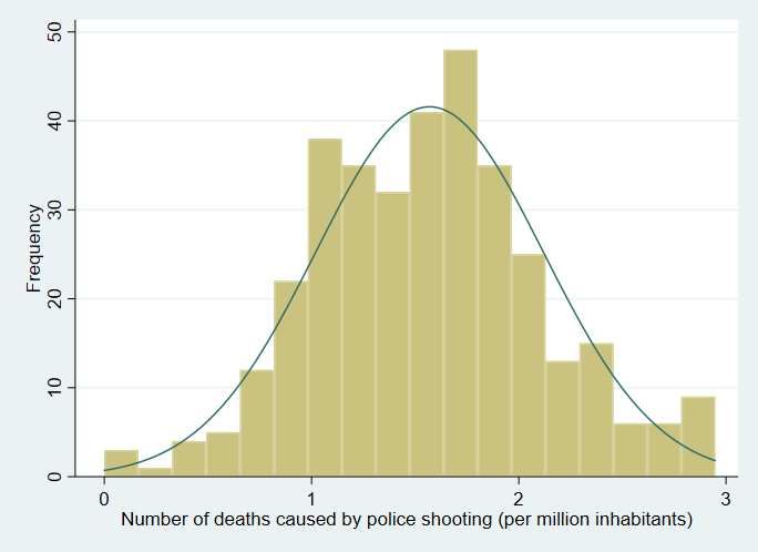
Figure A1: Distribution of the Dependent Variable (Pol shoot) before and after the
Yeo-Johnson Power Transformation (λ = 0.1384)
(a) Before
(b) After
23Table A1: Ancillary Information for Table 2 and Table 4
Ancillary Information for Table 2
(1) (2) (3) (4)
2014 1.089 1.105 1.055 1.081
2015 1.106 1.137 1.071 1.102
2016 1.149 1.190* 1.137* 1.148**
2017 1.224 1.285* 1.193* 1.220**
2018 1.363** 1.439** 1.308*** 1.344***
ln(α) 0.0540 0.0545
RESET Test 1 0.316 0.864 0.859 0.941
Mundlak Test 2 0.0555 0.3221
N. Obs. 300 300 300 300
Ancillary Information for Table 4
(5) (6) (7) (8)
2014 1.164 1.137 0.129 0.0943
2015 1.173 1.152 0.128 0.0985
2016 1.234** 1.199*** 0.188** 0.159**
2017 1.288** 1.264*** 0.199* 0.176**
2018 1.411*** 1.397*** 0.286** 0.265***
ln(α) 0.0463
RESET Test 1 0.405 0.976 0.880 0.659
2
Mundlak Test 0.3885 0.2854
N. Obs. 300 300 300 300
2013 as base year.
1) The RESET Test reports the p–value of the squared residuals.
2) The Mundlak Test reports the p-value of the joint significance test of the time
average of all regressors.
24You can also read


