Collie: COnfidence Level LImit Evaluator - V00.03.16
←
→
Page content transcription
If your browser does not render page correctly, please read the page content below
Collie:
COnfidence Level LImit Evaluator
V00.03.16
Wade Fisher
Fermi National Accelerator Laboratory
June 9th 2009 Collie Tutorial V000316 June 9th 2009 1
Outline
✗ Functional aspects of Collie
What is being calculated?
What do you need to calculate something?
What's going on behind the scenes?
✗ Operational aspects of collie
Creating CollieIO files
Calculations available in Collie
✗ Voiding your warranty
Abuse of the input assumptions
What should cross checks should be made?
June 9th 2009 Collie Tutorial V000316 2Content Warning
This tutorial covers a large range of concepts. Ideally this would be done in 2
3 separate presentations. If it feels a bit dense to you, you're not alone.
Many “advanced topics” are not included in this tutorial. The scope of this
presentation is based on the numerous questions I've received from users.
June 9th 2009 Collie Tutorial V000316 3Functional Aspects
of Collie
June 9th 2009 Collie Tutorial V000316 4Collie
✗ Collie is a software suite designed to generate semiFrequentist confidence
levels which are used to calculate a range of products
✗ The products available via Collie
pValues for TEST or NULL hypothesis. Or confidence level (CL) depending on which
book you read.
Cross section limit ratio: Signal scaling factor required to exclude at X% CL
Luminosity limit ratio: Lumi scaling factor required to exclude a model at X% CL
3Sigma evidence: Lumi scaling factor required to observe a model at 3Sigma
Cross section measurement: In the case of an excess in data, cross section scan or
floating cross section measurements
✗ The confidence level calculations available in Collie
CLfast: Fast, diagnostic tool ignoring systematics (!!not useful for real results!!)
CLsyst: Standard Gaussian smearing treatment for systematics
CLfit: Single binnedlikelihood fit, maximized over systematics
CLfit2: Double binnedlikelihood fit, maximized over systematics
June 9th 2009 Collie Tutorial V000316 5Some Definitions
✗ Compound hypotheses vs Simple hypotheses
Simple: The model probability distribution (PDF) is fully specified ( eg,
Gaussian with =3, =1.2 )
Compound: Indicates an underspecified PDF ( eg, Gaussian with =3 )
Operationally speaking: Your hypothesis has uncertainties (nuisance
parameters) which impact the predictions and you must account for this.
✗ Nuisance parameter
A parameter intrinsic to your MC model, but which is not the model
parameter you're trying to test. Can be a systematic uncertainty or a
theoretical parameter.
Example: Luminosity is known to about 6%. This means the TRUE signal
and/or background rates could be above or below what you predict in
your Monte Carlo.
Operationally speaking: To test outcomes of your compound model, you
must tranform to a simple hypothesis by assigning the nuisance
parameter a prespecified PDF (ie, a prior)
June 9th 2009 Collie Tutorial V000316 6The General Problem
✗ If possible, use data to distinguish two hypotheses:
✗ H0 null hypothesis: backgroundonly model, eg Standard Model
✗ H1 a test hypothesis: presence of a new particle, coupling, etc.
H0 is a compound hypothesis, with some set of nuisance parameters
H1 has the same form, but add model params and extra nuisance params
Simple Example: H0 describes the Standard Model background expectation for
the result of an analysis. Nuisance parameters can be luminosity, acceptance,
Standard Model cross section, etc...
H1 is the same as H0, but add a new physics signal. The model can be
parametrized by mass / cross section / etc, and extra nuisance parameters
come from signal acceptance, model parameters, etc...
June 9th 2009 Collie Tutorial V000316 7Complicating Factors
✗ The hypotheses, H1 & H0, are often subdivided according to final
states with unique signatures
Orthogonal (usually) search channels defined to maximize acceptance, isolate
high S/B regions, etc.
✗ The null hypothesis, H0, is the sum of several contributing Standard
Model processes
Nuisance parameters are generally correlated amongst backgrounds (and
signals!), but not always
✗ Discriminant distributions for expected and observed events are
binned into histograms
Discriminating variable can be an observable (eg, angular distribution) or
multivariable function (Neural Nets, likelihood ratios, etc).
Nuisance parameters can affect rates, shapes, or both. Many are
asymmetric and are not necessarily Gaussian.
June 9th 2009 Collie Tutorial V000316 8The SemiFrequentist Method
✗ A few words on the “AsFrequentistaspossible” treatment
Standard algorithm in all Collie calculation classes
✗ Given hypotheses, H1 & H0, we must simulate outcomes of repeated
experiments
Assume data is drawn randomly from a Poisson parent distribution
⇒ Generate pseudodata via random Poisson with mean value from expected
backgrounds (H0) or signalplusbackground (H1)
Systematics are a tricky Frequentist problem, so use a Bayesian model
⇒ Model uncertainties on nuisance parameters as Gaussiandistributed,
sample randomly for each pseudoexperiment
⇒ Vary nominal background prediction according to smeared values of
nuisance parameters, change mean of random Poisson each time
Generate ~20k pseudoexperiments for H1 & H0. This algorithm defines basis
of CLfast & CLsyst calculations.
June 9th 2009 Collie Tutorial V000316 9The Statistical Test
✗ Collie utilizes a negative Poisson loglikelihood ratio (LLR) test statistic to
evaluate statistical significance (test statistic = ordering rule)
Used to order data outcomes relative to each other in hypothesis significance
dij − sb ij d ij −bij
N C N bins
sb ij e bij e
Qs , b , d =∏ ∏ /
i=0 j =0 d ij ! d ij !
N C N bins
s ij
d =−2LogQ=∑ ∑ s ij −d ij ln 1
LLRs , b ,
i=0 j=0 bij
✗ LLR is linear in channels and bins: channel addition is natural formulation
✗ Implicitly imports info on the shapes of the parent distributions
✗ LLR value is evaluated for each set of pseudodata, generating distributions for
H1 and H0 hypotheses
Each outcome is ordered according to the LLR value
The frequency of relative outcomes defines confidence levels
June 9th 2009 Collie Tutorial V000316 10Same Thing in Pictures
Start by randomly smearing nominal
model according to nuisance parameters
Generate pseudodata via random
Poisson trials per histogram bin
Using pseudodata from random This process is repeated many times
Poisson trials, evaluate LLR (O(10k) for both H0 and H1. The
value and insert into histogram. observed LLR value is also evaluated.
June 9th 2009 Collie Tutorial V000316 11Example LLR Distributions
✗ Confidence levels are defined based on infinite integral of LLR distributions
Think of this as the “Prior Predictive Ensemble” of outcomes
CLb = fraction of HO pseudoexperiments less signallike than data
CLsb = fraction of H1 pseudoexperiments less signallike than data
1CLb
CLsb
Integrate LLR
distributions in
bkgdlike direction
June 9th 2009 Collie Tutorial V000316 12Example LLR Distributions
✗ Expected limits assume data = median expected background outcome
CLb = 50% if background is wellmodeled
“Expected” Data = Median Bkgd Outcome
1CLb
CLsb
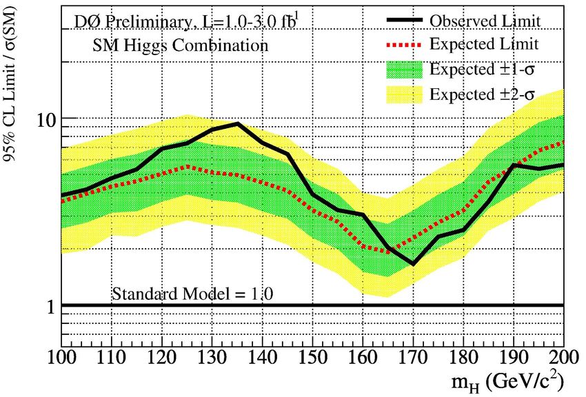
June 9th 2009 Collie Tutorial V000316 13Connecting with Standard LLR Plots
✗ We commonly plot LLR values as a function of a model variable, eg Higgs mass
Thes are just “overhead” views of LLR distributions at each Higgs mass
June 9th 2009 Collie Tutorial V000316 14Confidence Levels
✗ Now that we've introduced Confidence Levels, let's give definitions
Confidence interval: a range of values of a model parameter
Confidence level: the fraction of outcomes predicted to fall outside the
specified confidence interval
Statistically Speaking:
PROBx;, ( u(x) < < v(x) ) = 1 for all ,
x = test statistic, = parameter of interest (eg, xsec), = nuisance parameters
1- = confidence level, u(x) = lower limit, v(x) = upper limit
For example: Luminosity = 1000 ± 60 1/pb quoted at 1sigma
±60 1/pb defines the confidence interval
1sigma defines a confidence level of 68%
68% of possible true luminosity values lie within 940 < L < 1060 1/pb
June 9th 2009 Collie Tutorial V000316 15The CLs Statistic
✗ Given our confidence levels for our two hypotheses: CLsb and CLb
We want to describe confidence intervals relative to specific outcomes
1) Observed limits defined relative to observed data value
2) Expected limits defined relative to median background prediction
A strict Frequentist definition would use CLsb to define confidence interval
✗ The CLs prescription introduces an inherit dependence on the
background model description
CL sb 1CLb
CLs =
CL b
CLsb
New interval defined for 1CLs = 1
June 9th 2009 Collie Tutorial V000316 16The CLs Statistic
✗ Given our confidence levels for our two hypotheses: CLsb and CLb
We want to describe confidence intervals relative to specific outcomes
1) Observed limits defined relative to observed data value
2) Expected limits defined relative to median background prediction
A strict Frequentist definition would use CLsb to define confidence interval
✗ The CLs prescription introduces an inherit dependence on the
background model description
CL sb
CLs =
CL b
CLb
New interval defined for 1CLs = 1
Provides essential protection against
poor background modeling.
June 9th 2009 Collie Tutorial V000316 17A Higgs Search Example
✗ We begin by defining our confidence level requirement: CL = 95%
Given the SM Higgs cross section, very likely 1CLs < 95%
Thus, slowly increase signal rate until 1CLs = 95%
We thus define:
u(t) < SM Xsec < v(t) @ 95% CL
u(t) = 0, v(t) = cross section satisfying 1CLs
✗ In general, this method overcovers: CLsb < 5%
This is deemed acceptable based on our uncertain background model
✗ Because the lower limit=0, we use infinite integrals to define CL values
Thus, these CL values can be interpreted as pValues
June 9th 2009 Collie Tutorial V000316 18Marginalization
✗ Marginalization: broadening of nominal PDF via incorporation of systematics
✗ Compare “baseline” LLR (no systematics) to marginalized LLR distributions
No systematics: width of LLR dist given by Poisson uncertainty of samples
With systematics: width is proportional to quadrature sum of Poisson
uncertainty and systematics uncertainty 2 ∝ 2 2
tot Poisson systematics
Mean & observed LLR values remain the same, widths increase
Background CL increases and the ability to distinguish H1 & H0 decreases
Baseline LLR Distributions: CLfast Marginalized LLR Distributions: CLsyst
June 9th 2009 Collie Tutorial V000316 19Impact of Systematics
✗ Impact of systematics on limit depends on the statistics of the channel
Low statistics ⇒ Statistical uncertainty generally large WRT systematics
High statistics ⇒ Statistical uncertainty generally small WRT systematics
Statistics limited vs systematics limited analyses
✗ Can visualize by looking at ratio of limits with and without systematics
Convert to effective luminosity lost due to impact of systematics
✗ Painful, somewhat unavoidable, but we should be able to lessen this
Additional Luminosity Required for 95% CL exclusion due to Systematics
350 pb1 Results 1700 pb1 Results
High statistics
region: Hbb
Low statistics
region: HWW
June 9th 2009 Collie Tutorial V000316 20The Profile Likelihood
✗ To counteract the degrading effects of uncertainties on nuisance
parameters, we begin by defining the Profile Likelihood
Likelihood becomes a function of signal, bkgd, data, and nuisance
parameters
Maximizing the Profile Likelihood to a set of data points defines our “best fit”
for that data in a given hypothesis
L x∣R1 , S Two independent likelihood maximizations
Q= are performed over nuisance parameters
L x∣R0 , S parameters, one for each pseudoexperiment
R1 R0 : Physics parameters in H1 and H0, respectively
S : Nuisance parameters which maximize L for H1
: Nuisance parameters which maximize L for H0
S
June 9th 2009 Collie Tutorial V000316 21The Profile Likelihood
✗ Must define the best fit of our MC model to data
Assume prediction of N events per bin is a function of nuisance parameters
N syst Bi = nominally predicted bin content
B i Bi ∏ 1 i S k
k ik = fractional uncertainty
k=0 Sk = N sigma deviation from nominal
Assume data is Poisson distributed, derive constraint via statistical power of
data shape and systematic priors
N bins
P B i N syst
G k P(X) = Poisson PDF for X events
L=∏ × ∏ G(Y) = Gaussian PDF for systematic Y
i=0 P Di k =0 G 0k
Minimize Chi2 by varying Sk values
can “float” nuisance parameters by removing S2 constraint
B i
N bins N syst
= −2ln L = 2 ∑ B i−D i −D i ln ∑ S 2k
2
i=0 Di k =0
June 9th 2009 Collie Tutorial V000316 22The Profile Likelihood
✗ What's really happening?
Analyzer generates a background prediction based on MC, data (QCD), and
best guesses for central values of nuisance parameters
Many uncertainties on nuisance parameters are ~2040%!
Define “best fit to data” by minimizing our Poisson Chi2 over the central
values of the nuisance parameters
Each background source is varied independently according to uncertainties
Uncertainties can (should!) be given as a function of final variable
Correlations are important and rigorously maintained
Penalty term for deviations from nominal prediction eliminates free fit to data
⇒ constrains fit within errors of your best guess
Bi
N bins N syst
=2 ∑ Bi −Di −Di ln
2
∑ S 2
k
i=0 Di k=0
June 9th 2009 Collie Tutorial V000316 23Profile LH Fitting Example
Prefit: Sig: 0.81, Bkgd: 85.2, Data: 92
Postfit: Sig: 0.83, Bkgd: 89.3, Data: 92
June 9th 2009 Collie Tutorial V000316 24Profile LH Fitting Example
✗ Add another channel to the fit
Increased statistics impacts fit via correlated nuisance parameters
Prefit: Sig: 1.65, Bkgd: 440, Data: 436
Postfit: Sig: 1.65, Bkgd: 437, Data: 436
June 9th 2009 Collie Tutorial V000316 25Profiling Example
✗ Comparing “baseline” (ie, no systematics) and smeared LLR
distributions to those from the fitted profileLH prescription
Fitted background CL moves closer to 50% (better agreement with data)
Separation of S+B and BOnly hypotheses roughly the same
Width of LLR distributions grows slightly, but less than CLsyst prescription
NLLR Distributions
June 9th 2009 Collie Tutorial V000316 26Applying to the Calculation
✗ Two general ways of implementing the fit:
1) Fit each data distribution to a model (H1 or H0), calculate LLR
value after each fit
CLfit calculator class in Collie
Optionally remove regions with large S/B values to eliminate signal
contamination
Requires user input....beware....
1) Perform two fits to each data distribution (H1 & H0)
CLfit2 calculator class in Collie
Redefine LLR as Chi2 difference between fits As defined in
This is the more robust application, and no user input slides 1415
More powerful, but it's 2x slower...
LLRnew =2min H1 −2min H0
June 9th 2009 Collie Tutorial V000316 27CLfit Bin Exclusion
✗ Optionally remove bins with large signal contribution from fit
Assuming you're fitting to H0 hypothesis
Fit loses statistical power based on how many bins are removed
✗ Choice of window size is somewhat arbitrary, but needs care
Basic caveat: Exclude signals of the same size as the background fluctuation
(can't probe smaller than that!)
Window must grow as signal grows, taken care of automatically (ie, during
scaling procedure)
June 9th 2009 Collie Tutorial V000316 28The User Interface
to Collie
June 9th 2009 Collie Tutorial V000316 29The Starting Point
✗ What do you need to get started?
A final variable capable of distinguishing signal from background.
A signal hypothesis in the form of some acceptable simulation.
A background hypothesis, ideally separated into major background
components.
A data distribution.
Models for nuisance parameters.
✗ How should you package your inputs?
Collie can parametrize a model in 3D (eg, mass, width, branching fraction)
Collie can utilize 1D and 2D final variables, input as histograms.
Collie assumes ALL of your input distributions are normalized to the
expected number of events.
Nuisance parameters can be input in 3 separate ways:
✗ Constant, ±1 fractional uncertainties for each histogram bin (eg, Lumi)
✗ Histograms of nonconstant, ±1 fractional uncertainties per bin (eg, JES)
✗ Histogram resulting from varying the underlying nuisance parameter by ±1
June 9th 2009 Collie Tutorial V000316 30A bit more detail
✗ Signal normalization
If you normalize to expected numbers of events ( S=L0 ), limits are returned in
units of the input signal cross section 0 : R = Limit / 0
If you normalize to efficiency times lumi ( S=L ), limits will be returned in of cross
section
✗ Sign conventions for systematic uncertainties:
For fractional uncertainties, there's ambiguity so we have to choose a convention.
Ambiguity eliminated for alternative shapes.
Example for an asymmetric flat uncertainty of +10%, 7%
Alternative Shape Convention Fractional Uncertainty Convention
June 9th 2009 Collie Tutorial V000316 31The Collie User Interface
✗ To be flexible, Collie is composed of two parts:
File Creation: Interface classes designed to create formatted CollieIO files
used in all Collie calculations.
Users input data, MC, and nuisance parameter distributions for all
model parametrizations.
Internal “sanity checks” and closure tests are performed by Collie.
Resulting CollieIO files can be used, exchanged, or combined to generate
a calculational product.
Calculations: Classes which perform standardized calculations based on
user input files.
Users provide formatted CollieIO files and design an executable for the
calculation.
Calculations can be CPU intensive, so batch submission is
recommended.
June 9th 2009 Collie Tutorial V000316 32Getting/Building Collie
✗ Collie can be found in d0cvs
For a tagged version of Collie: cvs co r V000316 collie
For the most recent version of Collie: cvs co A collie
untagged versions aren't guaranteed to be safe...
✗ Collie does not use the SRT gmake, but comes with its own makefile. To build
collie:
1) cd collie
2) source setup_Collie.tcsh (or use the bash version. syntax depends
on your shell, edit as needed)
3) make (ROOT may complain. Just ignore it. ROOT isn't a C++ authority!)
✗ A successful build will create the following files:
collie/lib/libCollieIO.so collie/lib/libCollieLimit.so
collie/examples/collieIOmaker.exe collie/examples/collieLimitCalc.exe
collie/examples/collieXsecCalc.exe collie/examples/resultsFileCombiner.exe
June 9th 2009 Collie Tutorial V000316 33Creating a CollieIO File
✗ The first step is creating an input file for calculations
Adapted from collie/examples/collieIOexample.cc
int main(int argc, char* argv[]) {
/////////////////////////////////////////
///Create IO file with input parameters
/////////////////////////////////////////
CollieIOFile* cfile = new CollieIOFile();
cfile>initFile("exampleCollieIOfile.root", "Test Channel"); //outputfile and channel name
cfile>setInputHist(0.0,1.0,20); //Define your input histograms
cfile>setCutoffs(0.0,1.0); //Option to define physical cutoffs
cfile>setRebin(1); //Option to rebin histograms to a coarser binning
cfile>setSmooth(false); //Option to smooth histograms
//Define backgrounds
vector bkgdNames;
bkgdNames.push_back("Bkgd1");
bkgdNames.push_back("Bkgd2");
cfile>createChannel(bkgdNames);
//Get your input histograms from somewhere (made up at random in the example)
//or get them from a file:
// TFile infile("myInputFile.root");
// TH1D* data = (TH1D*)infile.Get("data");
// TH1D* signal = (TH1D*)infile.Get("signal");
// TH1D* bkgd1 = (TH1D*)infile.Get("bkgd1");
June 9th 2009 Collie Tutorial V000316 34Creating a CollieIO File
✗ Continued from previous slide...
//Backgrounds are passed in via vector
vector vbkgd;
vbkgd.push_back(bkgd1);
vbkgd.push_back(bkgd2);
//Alpha parameters only matter when smoothing is utilized
// Input values don't matter if you're not smoothing.
// Don't smooth unless you know what you're doing.
vector valpha;
//Each parameter point has a signal histo, data histo, and an array of backgrounds...
// Smoothing parameters are also passed in.
cfile>createMassPoint(100, data, sig, 1, vbkgd,valpha);
//Add systematics...either flat or by shape (ie, function of final variable)
// if by shape, must supply a histogram of the values in percent(%) fluctuations...
// Signal requires no index, but backgrounds must be specifically indexed (0>N bkgds)
cfile>createFlatSigSystematic("Lumi",0.06,0.06,100);
cfile>createShapeSigSystematic("SigShape",sigSystP,sigSystN,100);
cfile>createFlatBkgdSystematic(0,"Lumi",0.06,0.06,100);
cfile>createFlatBkgdSystematic(1,"Lumi",0.06,0.06,100);
///store channel
cfile>storeFile();
}
June 9th 2009 Collie Tutorial V000316 35Output of CollieIO Example
✗ Summarized result obtained after running collie/examples/collieIOmaker.exe
>>./collieIOmaker.exe
==>Created mass point 100 Report on I/O procedures, look for error
warnings here
Mass: 100
Data: 451
Signal: 7.504 Checksum integrals of input histograms.
Bkgd: Bkgd1, 150.00
Bkgd: Bkgd2, 299.876 “Sanity check” that you get out what
Allbkgd: 449.88 you put in
Output files:
fv_XY.root is a histogram file
==>Saving inspection histos to representing everything stored in the
fv_exampleCollieIOfile.root
collieIO input file for your inspection.
This is not your colleIO file!
==>Saving channel data to
exampleCollieIOfile.root....
XXX.root is your collieIO input file
June 9th 2009 Collie Tutorial V000316 36CollieIO Systematics API
✗ There are six different methods for adding systematics at the CollieIO step,
three each for signal and background:
Flat systematics: CollieIOFile::createFlatSigSystematic(...) and
CollieIOFile::createFlatBkgdSystematic(...). Use this for things like luminosity where
every bin gets the same uncertainty value.
UserDefined shapedependent systematics: CollieIOFile::createSigSystematic(...) and
CollieIOFile::createBkgdSystematic(...). Users may define any fractional uncertainty
shape that they wish.
Shapedependent systematics: CollieIOFile::createShapeSigSystematic(...) and
CollieIOFile::createShapeBkgdSystematic(...). Users pass Collie alternative final
variable shapes for systematic uncertainties (ie, the shapes you'd get for +/1 sigma
for a given systematic). There are many modification choices available for these
methods, please read the instructions.
Please read the detailed usage instructions for each method in
collie/io/include/CollieIOFile.hh
June 9th 2009 Collie Tutorial V000316 37CollieIO Warnings and Errors
✗ Collie automatically checks for errors in the following areas:
Statistical uncertainties: Basic sanity checks, such as “Did you call TH1D::Sumw2()?”,
“Are your statistical uncertainties larger than bin content?”, etc.
Systematic uncertainties: Do you have any systematics larger than ~50%? If so, you
may consider a LogNormal PDF. Otherwise, you may have the wrong systematics.
Systematic uncertainties: Are your shape systematics dominated by noise? If so,
Collie will automatically flatten these.
Systematic uncertainties: Did you accidentally put the same shape systematic
histogram in twice for both positive and negative fluctuations? This is a valid use
case and Collie will interpret this as a symmetric fluctuation. But you'll still get a
warning.
Histogram contents: Do you have underflow or overflow? Collie ignores
under/overflow.
Histogram contents: Do you have bins with nonzero signal, nonzero data, and zero
background? If so, you don't need Collie. You need to call a press conference or
reconsider your background model. Collie will merge these bins to the nearest
neighbor with highest S/B content.
June 9th 2009 Collie Tutorial V000316 38Calculations Available in Collie
Recall our definition of CLs
CL sb
✗
CLs =
Defends against false discovery when
dataExample Limit Calculation
✗ Once you've created a CollieIO file, you can calculate something...
Adapted from collie/examples/exampleLimitCalculation.cc
void loadLimits(char* outfile, char* m) {
//What mass point are we interested in
int mass = atoi(m);
//Open the CollieIOFile created in I/O example step...
char options[1024]; bool ok = true;
////Specify the channel name given in the I/O step
sprintf(options,"name='%s'","Test Channel");
//Pass this information to the CollieLoader to extract the channel info
CollieLoader loader;
if (!loader.open(“exampleCollieIOfile.root”,options)) {
std::coutExample Limit Calculation
✗ Continued from last slide...
// This is the class for computing cross section limits
CrossSectionLimit csLim;
csLim.setup(&clcompute); //Pass in the computer you chose
csLim.setVerbose(false);
csLim.setCLlevel(0.95); //Set to 0.95 for 95% CL calculation (default = 0.95)
csLim.setPrecision(0); //0 is lowest(fastest), 4 is highest(slowest)
csLim.calculateExpected(true); //toggle on/off expected/observed limits
csLim.calculateObserved(true); // to get speed things up if you wish
//tell the container what point you're working on
clresults.reset(v1[i],v2[i],v3[i]);
//Extract the signal & background distributions associated with this point
SigBkgdDist* sbd=loader.get(v1[i],v2[i],v3[i]);
//calculate Confidence Levels
clcompute.calculateCLs(*sbd,clresults,CLcompute::LEVEL_VERYFAST);
//report your results for interested observers
clresults.print();
//Calculate a cross section limit...
//These results are reported in the factor by which you must
//multiply your nominal signal cross section to obtain a 95% CL
//upper limit for this model... IE, multiply this factor by
//your model xsec to get your limit in barns
csLim.calculate(*sbd,clresults);
//report your results for interested observers
csLim.print();
}
June 9th 2009 Collie Tutorial V000316 41Output of Limit Calculation
✗ Calculating limits for mH=105 from the example inputs
./collieLimitCalc.exe myOutput.root 100 Output stored in ROOT format in specified
file, set mass point to 1 to get all in the
input file
****************************************:
CLcompute Results:
CLs_obs: 0.6462, CLs_med: 0.7237
CLsb_obs: 0.2235, CLsb_med: 0.1381 Report of nonscaled CL calculations
CLb_obs: 0.6316, CLb_med: 0.5168
LLRobs: 0.5406, LLRb: 1.1609, LLRsb: 1.2352, lumifactor: 3.249
LLRb_m2s: 5.1118, LLRb_m1s: 3.2550
LLRb_p1s: 0.9013, LLRb_p2s: 3.1823
****************************************:
****************************************:
CrossSectionLimit calculator results::
==>CL level: 0.9500, N sigma: 0
==>Accuracy: 0.0010, Precision: 0 Report of limit calculation
==>Scaling factor Exp: 1.900, Obs: 2.181
****************************************:
14.594 sec run time Job timer
June 9th 2009 Collie Tutorial V000316 42Combining Channels
✗ If you wish to combine two or more channels:
Simply append appropriate distributions from the channels
✗ When combining channels, you must make sure that correlations amongst
systematics are properly specified
Collie will correlated all systematics whose names are identical. Eg, “lumi”
and “lumi”, but not “Lumi” and “lumi”.
CollieLoader loader;
if (!loader.open(“collieIOfile1.root”,options)) {
ok = false;
}
CollieLoader loader2;
if (!loader2.open(“collieIOfile2.root”,options)) {
ok = false;
}
if(!ok) return;
...Normal calculation setup...
//Extract the signal & background distributions associated with this point
SigBkgdDist* sbd1=loader1.get(v1[i],v2[i],v3[i]);
SigBkgdDist* sbd2=loader2.get(v1[i],v2[i],v3[i]);
//Append the two distributions
sbd1>append(*sbd2);
June Collie Tutorial V000316
9th 2009 with your calculations...
...Continue 43Combining Channels, ctd.
✗ When combining channels, you must make sure that correlations amongst
systematics are properly treated
Collie will correlated all systematics whose names are identical. Eg, “lumi”
and “lumi”, but not “Lumi” and “lumi”.
✗ Users with many input channels may wish to used “condensed” IO files
Use the IO condenser program: examples/collieIOcondenser.cc
✗ Batch submission script:
collie/limit/macro/CollieBatch.perl
✗ Fitting macros (more on this later):
collie/limit/macro/fitResults.C
collie/limit/macro/fitXsec.C
June 9th 2009 Collie Tutorial V000316 44Additional Tools
✗ Plotting macros for ROOT output of limit calculations:
collie/limit/macro/plotCLb.C
collie/limit/macro/plotFactor.C
collie/limit/macro/plotCL.C
collie/limit/macro/plotLLR.C
✗ Batch submission script:
collie/limit/macro/CollieBatch.perl
✗ Fitting macros (more on this later):
collie/limit/macro/fitResults.C
collie/limit/macro/fitXsec.C
June 9th 2009 Collie Tutorial V000316 45Viewing LLR Distributions
✗ You may wish to directly view your LLR distributions. Add the following lines
to add histograms of LLR distributions to the output file.
//calculate CLs...
clcompute.calculateCLs(*sbd,clresults,CLcompute::LEVEL_STANDARD);
//report your results for interested observers...
clresults.print();
//Add the following lines...
int bins = 5000; double min = 50; double max = 50;
TH1D* sigLLR = clcompute.getLLRdist_sb("LLR_SB",bins,min,max);
TH1D* bkgLLR = clcompute.getLLRdist_b("LLR_B",bins,min,max);
TH1D* LLRd = new TH1D("LLR_D","LLR_D",bins,min,max);
TH1D* LLRsigma1 = new TH1D("LLR_B_1sigmas","LLR_B_1sigmas",bins,min,max);
TH1D* LLRsigma2 = new TH1D("LLR_B_2sigmas","LLR_B_2sigmas",bins,min,max);
LLRd>Fill(clresults.llrobs);
LLRsigma2>Fill(clresults.llrb_m2s);
LLRsigma1>Fill(clresults.llrb_m1s);
LLRsigma1>Fill(clresults.llrb_p1s);
LLRsigma2>Fill(clresults.llrb_p2s);
The above instructions provide
nonscaled LLR distributions
June 9th 2009 Collie Tutorial V000316 46Extracting ±1,2 Sigma Bands
✗ A pleasing limit presentation feature is the
1,2 sigma bands around the expected limit
A common misconception: “This is the error on
the limit”.
There is no error on a limit unless you made a
mistake! It's just a calculation.
✗ The true interpretation is, “What limit
would I get if the data disagreed with
background to this degree?”
Determined by recalculating limits for 4 2
different outcomes 1 -0
Bands enclose 68% and 95% of background
outcomes, respectively. -0
// This is the class for computing cross section limits
CrossSectionLimit csLim;
csLim.setup(&clcompute); //Pass in the computer you chose
csLim.setNSigma(2); //Calculate +2 sigma
//csLim.setNSigma(1); //Calculate 2 sigma
June 9 2009
th
Collie Tutorial V000316 47Common Beginner Mistakes
✗ Problem: The CollieIO step doesn't report the correct histogram integrals!
Cause 1: Check that you specified the correct histogram parameters when
you made the input files (see slide #24)
Cause 2: If you're using smoothing did not specify valid smoothing
parameters (see next slide)
✗ Problem: The CollieIO step complains about my systematics histograms!
Cause 1: Collie will complain if you try to add a histogram that doesn't
match the specified histogram parameters or is NULL.
✗ Problem: The calculation step complains when I load my input file!
Cause 1: Did you specify the correct channel name for the input file?
Cause 2: If you're appending two channels, do they have the same channel
name?
June 9th 2009 Collie Tutorial V000316 48Safety Net for Beginners
✗ The Collie Novice Flag
By default, Collie sets a flag defining the user as a novice
This flag will prevent you from using the following aspects:
Statistical Uncertainties, Smoothing, Interpolation, & Fitting
✗ No Statistical Uncertainties? Why??
By default, Collie assumes you either forgot, screwed up, or don't understand your
statistical uncertainties.
By default, ROOT doesn't do a proper accounting of statistical uncertainties.
If you turn off the novice flag, Collie will test your statistical uncertainties for
appropriateness. Check for warnings, but the ball's in your court....
Unsetting the Novice Flag
//Unsetting the novice flag in IO code
CollieIOFile* cfile = new CollieIOFile();
cfile>initFile("exampleCollieIOfile.root", "Test Channel"); //outputfile and channel name
cfile>setNoviceFlag(false);
//Unsetting the novice flag in calculation code
CLfast clcompute; //The CLfast computation uses no systematics
clcompute.setNoviceFlag(false);
//Use of histogram statistical uncertainties can be enabled as follows:
clcompute>useHistoStats(true);
June 9th 2009 Collie Tutorial V000316 49Potential Hazards in Collie
✗ Smoothing
Collie contains an algorithm for histogram smoothing as an alternative to the sketchy
one available in ROOT.
⇒ If you're using Collie's smoothing algorithm, I assume you know what you're doing.
If you don't, contact me.
✗ Histogram binning
Collie assumes you know what you're doing when you specify how many bins to use in
your final variable.
⇒ Correct binning is intrinsically linked to the resolutions of observables and the
statistics of your sample. BINNING IS NOT AN OPTIMIZABLE VARIABLE FOR
LIMIT CALCULATIONS!!
✗ Data/MC agreement
Collie assumes you've studied your backgrounds and you have reasonable agreement
with data. Collie will happily calculate limits, etc for input channels that have no
business trying to do so.
⇒ Perfect Data/MC agreement isn't mandatory, but you should doublecheck the
output of the CollieIO step to ensure you agree with what is in the input file
June 9th 2009 Collie Tutorial V000316 50Potential Hazards in Collie
✗ Systematic Uncertainties
If your systematics are larger than ~2530%, you probably shouldn't be using the
default Gaussian PDF for systematic uncertainties due to truncation issues
⇒ If you believe your event rate has a probability of 0 for 0 events, then switch to the
log normal parametrization Specify this in the collieIO step: see below.
⇒ If you have at least 1 MC event in a bin, it's hard to motivate a nonzero probability for
0 evts
✗ Systematic Uncertainties
How well do you believe your uncertainty
anyway? Does 100% uncertain make
sense?
⇒ A better solution might be to remove the PDF
constraint, assign a sensible uncertainty,
and let a poorly known systematic “float”.
//Specify Log Normal for a systematic
cfile>setLogNormalFlag("YourSystName", true, 100);
//remove the PDF constraint for a systematic
cfile>setBkgdFloatFlag(0, "systName", true,100);
June 9th 2009 Collie Tutorial V000316 51Systematics: Fitting vs PseudoExperiments
✗ A common misconception:
“If I overestimate my uncertainties, it's OK because Collie will just find the true value
for me.”
✗ For a single fit to a single set of data or pseudodata, this is true.
MINUIT determines the covariance matrix by sampling the chi2 response functions in
each eigenvector direction. This results in a perfit estimate of uncertainty size.
✗ However, all of your pseudoexperiments are drawn from the systematic
uncertainty priors that you've supplied.
If you specify 100% uncertainty when you really mean 20%, your LLR distributions will
be 5x wider than they should. Thus, your sensitivity is necessarily degraded.
June 9th 2009 Collie Tutorial V000316 52Fit Quality Testing
An important issue for users to understand
Collie runs fixed algorithms designed for a broad range of HEP problems. In the case of
fitting, Collie makes the implicit assumption that the user has constructed an
appropriate fit model. Thus, it is the user's responsibility to generate and
understand their backgrounds, systematics, and correlations.
June 9th 2009 Collie Tutorial V000316 53Testing your Fit
✗ The Collie fitting test can be performed after CollieIO file creation
Just the additional lines to be added to the example calculations.
The fit test can be run at the same time as the calculation, but I recommend testing
before calculating.
#include
//Add before the masspoint loop
FitTest fitTest;
fitTest.setIterations(2000); //Determines how many trials will be run in the test
fitTest.testPE(true); //Toggles whether to test pseudoexperiments
//Add inside the masspoint loop
fitTest.runTest(sbd,sigLLRcut); //Pass the SigBkgdDist you want to test. Appending is OK.
//The “sigLLRcut” is the same cutoff used by CLfit. If
//you're not using CLfit, then you can ignore this.
✗ The fit test creates an output file with information about your fit
Global information about the input channels
Response information from MINUIT about fit convergence
“Best fit” values for all your nuisance parameters when fit to data
Individual nuisance parameter response and pull functions
June 9th 2009 Collie Tutorial V000316 54Testing your Fit
✗ Examine your fit test results using the macro
collie/limit/macro/fitResults.C
==>Detailed instructions are included inside the macro
>> root l
root [0] .L fitResults.C
root [1] makePlots("fitTest.root")
Before fit========> Sig: 335.7244, Bkgd: 12051.4437, Data: 12437.0
After S+B fit=====> Sig: 245.7548, Bkgd: 12187.0099, Data: 12437.0
After BOnly fit==> Sig: 341.4754, Bkgd: 12427.3283, Data: 12437.0
Sideband data: 9171, Ignored data: 3266
Sideband bins: 27, Ignored bins: 23
✗ Basic report includes:
Sig, Bkgd, & Data integrals before and after fitting
Data integral that would be included/ignored in a CLfit (singlefit) calculation
Bins that would be included/ignored in a CLfit (singlefit) calculation
June 9th 2009 Collie Tutorial V000316 55Testing your Fit
✗ Input Distribution Diagnostics
Comparison of input distributions:
Background, Signal+Bkgd, & Data
Report on # of Gaussian sigmas per
bin compared to data. Available
before and after fits.
June 9th 2009 Collie Tutorial V000316 56Testing your Fit
✗ MINUIT Diagnostics
Number of MINUIT iterations
required for convergence. S+B fit
should take a bit more.
MINUIT fit status. Anything other
than 3 is bad news....
June 9th 2009 Collie Tutorial V000316 57Testing your Fit
✗ Fit diagnostics
Best fit central values for nuisance
parameters. Reported in units of N
sigma.
Histogram of Log(1+S/B) for data,
nominal background, best fit
background, and data.
June 9th 2009 Collie Tutorial V000316 58Testing your Fit
✗ Persystematic diagnostics
Comparison of nominal, best fit, and
+/ 1 sigma fluctuations.
Pull functions for smeared MC fits to
data (A), nominal MC fits to pseudo
experiments (B), 1D floating Chi2
response function (C), and associated
statistics.
June 9th 2009 Collie Tutorial V000316 59Testing your Fit Pull function for fits to data: An N Pull function for fits to pseudodata: An N dimensional systematic test. By dimensional systematic test. Nominal MC is fit to injecting unit Gaussian (or log pseudoexperiments. This plot indicates how normal) distributions, this plot much each systematic is being moved to shows the resulting distribution of accommodate the range of pseudoexperiment systematic values after fitting to outcomes. Vary narrow pulls usually correspond data. 1sigma in and 1sigma out to a flat chi2 response (see below). means no constraint in data. Widths less than 1.0 indicate a datadriven constraint on the systematic. The chi2 response function: while holding all other systematics fixed, vary this parameter from N sigma to +N sigma. Curvature provides info on how much of this change your data will accommodate. Location of minimum provides info on relative data/MC agreement. June 9th 2009 Collie Tutorial V000316 60
Extrapolated
Tips & Tricks
P17 Limits
✗ Speeding things up:
1) You can calculate expected and observed limits in separate jobs. Recombine output
files with collie/examples/resultsFileCombiner.exe:
./resultsFileCombiner.exe newFile.root listOfExpFiles.txt listOfObsFiles.txt
2) When fitting, MINUIT's Fortran code needs to output messages (fort.99 file). You
can speed up I/O by creating a symbolic link to /dev/null: ln s /dev/null fort.99
3) Collie's search algorithm starts at a signal rate of 0.75. If your limit will be far from
this, you can speed up the search by seeding with a value close to what you might
expect
// This is the class for computing cross section limits
CrossSectionLimit csLim;
csLim.setup(&clcompute); //Pass in the computer you chose
csLim.setSearchSeed(10); //Speed things up if your limit will be closer to 10 than 1
✗ Use baby steps to understand how your inputs behave with fitting:
1) Start with CLfast: check limits and LLR plots. Do things look OK?
2) Next try CLsyst: check limits and LLR plots. Still OK?
3) RUN A FIT TEST!! Do things look sensible?
4) Run with CLfit2: check limits and LLR plots for compatibility with (1) & (2)
June 9th 2009 Collie Tutorial V000316 61Extrapolated
Wrap P17
Up Limits
✗ Collie is a software package for the statistical treatment for a system of
N compound analysis channels with implicit correlations amongst
uncertainties on nuisance parameters
Documented via DZero note (#4975 & #5309) ...not complete...
Available within DZero CVS
Examples available within the package
✗ Statistics EB review of Collie will hopefully be done very, very soon
✗ Users are encouraged to get started using Collie
Try to not use as a “black box”. Knowing what to expect will help
eliminate mistakes.
Expect EBs to want to see sensible results from Collie's fitting tests!
Feedback and questions are very welcome.
June 9th 2009 Collie Tutorial V000316 62You can also read