Bayesian forward modelling of cosmic shear data - arXiv.org

MNRAS 000, 1–11 (2020) Preprint 22 January 2021 Compiled using MNRAS LATEX style file v3.0

 Bayesian forward modelling of cosmic shear data
 Natalia Porqueres,1★ Alan Heavens,1 Daniel Mortlock,1,2,3 and Guilhem Lavaux4
 1 Imperial
 Centre for Inference and Cosmology (ICIC) & Astrophysics group, Imperial College, Blackett Laboratory,
 Prince Consort Road, London SW7 2AZ, UK
 2 Department of Mathematics, Imperial College London, London, SW7 2AZ, UK
 3 Department of Astronomy, Stockholm University, Albanova, SE-10691 Stockholm, Sweden
 4 CNRS & Sorbonne Université, UMR7095, Institut d’Astrophysique de Paris, F-75014, Paris, France
arXiv:2011.07722v2 [astro-ph.CO] 21 Jan 2021

 Accepted 21/01/2021. Received 20/01/2021; in original form 13/11/2020

 ABSTRACT
 We present a Bayesian hierarchical modelling approach to infer the cosmic matter density field, and the lensing and the matter
 power spectra, from cosmic shear data. This method uses a physical model of cosmic structure formation to infer physically
 plausible cosmic structures, which accounts for the non-Gaussian features of the gravitationally evolved matter distribution and
 light-cone effects. We test and validate our framework with realistic simulated shear data, demonstrating that the method recovers
 the unbiased matter distribution and the correct lensing and matter power spectrum. While the cosmology is fixed in this test,
 and the method employs a prior power spectrum, we demonstrate that the lensing results are sensitive to the true power spectrum
 when this differs from the prior. In this case, the density field samples are generated with a power spectrum that deviates from the
 prior, and the method recovers the true lensing power spectrum. The method also recovers the matter power spectrum across the
 sky, but as currently implemented, it cannot determine the radial power since isotropy is not imposed. In summary, our method
 provides physically plausible inference of the dark matter distribution from cosmic shear data, allowing us to extract information
 beyond the two-point statistics and exploiting the full information content of the cosmological fields.
 Key words: cosmology:large-scale structure of Universe – methods:data analysis – weak gravitational lensing

 1 INTRODUCTION 1997; Jain & Seljak 1997; van Waerbeke et al. 1999; Schneider &
 Lombardi 2003; Takada & Jain 2003; Vafaei et al. 2010; Kayo et al.
 As light from distant galaxies propagates through the Universe, it is
 2013). While some approaches to access the non-Gaussian infor-
 deflected by the gravitational field induced by the large-scale struc-
 mation are based on measuring high-order correlations (Bernardeau
 tures. This deflection results in a coherent distortion of observed
 et al. 2003; Pen et al. 2003; Jarvis et al. 2004; Semboloni et al. 2011;
 galaxy images, inducing small changes in the ellipticity of observed
 van Waerbeke et al. 2013; Fu et al. 2014), peak counts (Jain & van
 galaxies, which is known as cosmic shear. The weak gravitational
 Waerbeke 2000; Dietrich & Hartlap 2010; Maturi et al. 2011; Marian
 lensing effect is sensitive to the geometry of the Universe and the
 et al. 2012; Pires et al. 2012; Cardone et al. 2013; Lin & Kilbinger
 growth of cosmic structures, making it a powerful probe to study the
 2015; Liu et al. 2015b,a; Kacprzak et al. 2016; Petri et al. 2013; Peel
 matter distribution and the nature of dark matter and dark energy
 et al. 2017) or using machine learning (Gupta et al. 2018), they rely
 (see e.g. Kilbinger 2015, for a review).
 on summary statistics that do not capture all the information and
 The next-generation surveys like Euclid (Euclid Collaboration
 whose distributions are not well known.
 et al. 2020), Roman Space Telescope (Spergel et al. 2015) and the
 Rubin Observatory (LSST Science Collaboration et al. 2009) will Capturing the full information content of the large-scale structure
 provide unprecedented precision in cosmic shear measurements, per- requires a field-based approach to infer the matter distribution from
 forming wide-field cosmic shear surveys and measuring large and observations. Böhm et al. (2017) presented a maximum likelihood es-
 small scales. Harvesting the information from these data sets will timator to reconstruct the matter density field from cosmic shear data,
 present a challenge. Many of the current cosmic shear analyses focus assuming a log-normal distribution for the density. The log-normal
 on extracting information from the correlation function or the asso- distribution reproduces the one- and two-point statistics but fails to
 ciated power spectrum (Kitching et al. 2011; Heymans et al. 2013; reproduce higher-order statistics. Alsing et al. (2016, 2017) presented
 Kitching et al. 2014, 2015; Alsing et al. 2016; Kitching et al. 2016; a Bayesian hierarchical inference scheme to jointly infer shear maps
 Hildebrandt et al. 2017; Troxel et al. 2018; Hikage et al. 2019; Tay- and the corresponding power spectra, assuming Gaussian statistics
 lor et al. 2019). These analyses capture the two-point statistics, but of the shear field. From a Bayesian perspective, assuming a Gaussian
 they do not fully capture the non-Gaussian information encoded in distribution for the shear field is a well-motivated prior since it con-
 the filamentary features of the matter distribution (Bernardeau et al. stitutes the maximum entropy prior once the mean and covariance are
 specified. However, more information coming from physics is avail-
 able, and the Gaussian assumption is sub-optimal. In this work, we
 ★ n.porqueres@imperial.ac.uk address this limitation by including a gravity model in the Bayesian

 MNRAS 000, 1–11 (2020)

2 N. Porqueres et al.
 2 THE DATA MODEL
 The effect of weak gravitational lensing on a source can be described
 by two sky fields: the spin-2 shear, , which describes the distortion
 in the shape of the image, and the scalar convergence field, , which
 describes the change in angular size. These two fields are related to
 the lensing potential, , by
 1 ¯
 = , (1)
 2
 1
 = 1 + 2 = , (2)
 2
 (see e.g. Kilbinger 2015), where 1 and 2 are the components of
 the shear distortion parallel and at /4 to the coordinate axes, and
 = + is the complex derivative on the sky, assuming the
 flat-sky approximation.
 To connect the shear fields to the 3D dark matter distribution, we
 implemented a line-of-sight integration using the Born approxima-
 tion, integrating along unperturbed paths. First, we generate conver-
 gence fields by integrating along the line-of-sight with the corre-
 sponding lensing weights as
 3 02 Ω ∫ lim 
Figure 1. Hierarchical representation of the BORG inference framework for ( ) = ( ) ( , ), (3)
the analysis of cosmic shear data. Primordial fluctuations ic encoded in a a set 2 2 0 ( )
of Fourier modes at ≈ 1000 are obtained from the prior ( ic |Ω), where Ω where is the position on the sky, is the comoving distance, lim is
represents the cosmological parameters. These initial conditions are evolved
 the limiting comoving distance, is the final density field and
using the gravity model M ( ic ), which provides the evolved density f . The
 0 − 
 ∫ lim
evolved density and the redshift distribution of sources ( ) are then used to
compute the convergence field for each tomographic bin , ( , ( )). ( ) = 0 ( 0 ) 0 , (4)
 
From the convergence, we compute the cosmic shear 1 , 2 in the flat-sky
approximation. ˆ1 , ˆ2 indicate the observational data. Purple boxes indicate where ( ) is the source galaxy distribution. In our discrete imple-
deterministic transition while green boxes are probability distributions. mentation, this becomes

 3 02 Ω ∑︁
 2
 
 2
 h ∑︁ ( − ) i Δ 
 = ( )Δ . (5)
 2 2 =0 = 
hierarchical model. For this, we build on the Bayesian Origin Re- The index labels the tomographic bin and the subindices indi-
construction from Galaxies (BORG, Jasche & Kitaura 2010a; Jasche cate the 2D pixel on the sky, whose size is chosen to include typically
& Wandelt 2013a; Lavaux et al. 2019) framework, which employs many sources. The sum index indicates the slice in the radial di-
a physical description of the dark matter dynamics and allows us to rection, at a comoving distance . 2 is the total number of voxels
sample from the initial conditions, which are accurately described along the radial axis. The voxels have a length of Δ . is the
by Gaussian statistics. With this more complex data model, we get a 3D dark matter overdensity at a scale factor . The comoving radial
better representation of the data, and we can extract information be- distance indicates the distance to the source plane. The redshift
yond the two-point statistics, exploiting the full information content distribution of sources for each tomographic bin is given by ( ).
of the shear fields. In this initial proof-of-concept work, we focus on testing the infer-
 One of the main challenges in the analysis of cosmic shear based on ence and investigating the extent to which the 3D density field, and
estimating the power spectrum is accounting for the masked regions the 3D matter power spectrum, can be inferred from 2D shear maps.
within the survey area (see, e.g. Chon et al. 2004; Brown et al. 2005; For these tests, we used a simplified scenario, assuming flat-sky and
Smith 2006). Our forward modelling approach circumvents these distant observer approximations. In future work, we will drop these
difficulties associated with the survey mask. Although the data do approximations and consider the projection effects.
not provide information about the fields in the masked regions, the In the flat-sky approximation, we can obtain the shear values from
dynamical model still provides probabilistic information about the the convergence field. On a flat-sky, the shear and the convergence
shear and density fields that are physically possible in those regions. are related in Fourier space. We, therefore, use a discrete Fourier
In our method, the masked regions are treated as pixels with infinite transform (DFT) to obtain the shear values as
noise, circumventing the need to treat unobserved areas as being cut " #
 2
from the analysis. −1 ( + ) 
 = DFT DFT( ) , (6)
 The paper is organised as follows. Section 2 describes the data 2 + 2 
model for the cosmic shear and the likelihood. Section 3 gives an
overview of the Bayesian inference framework, BORG, as required where ® = ( , ) is the wave-vector written as a complex quantity.
for this work. In Section 4, we described the simulated data employed Since the convergence is also computed as part of the hierarchical
in testing and validating the method. The results are presented in model, this method has the advantage that it can analyse reduced
Section 5, showing that the method provides unbiased matter density shear,
fields. In Section 7, we discuss the effect of the prior power spectrum 
in the results. Finally, Section 8 summarises the results. = , (7)
 1− 

MNRAS 000, 1–11 (2020)

Bayesian forward modelling of cosmic shear 3

Figure 2. Redshift distributions of sources for the four tomographic bins Figure 3. Mask used to generate the mock data. The masked regions, with no
considered in this analysis. contributing sources, are indicated in black. There are two different scales,
 corresponding to non-observed regions and bright stars.

which, rather than the shear alone, controls the shape distortion.
 To analyse cosmic shear observations in our Bayesian framework,
we now built a likelihood based on this data model. We assume inferring the non-linear spatial dark matter distribution and its dy-
Gaussian pixel noise for the shear, corresponding to a negative log- namics from cosmological data sets. The underlying idea is to fit
 ˆ ), that can then be written as
likelihood, L = − log ( | full dynamical gravitational and structure formation models to ob-
 servations. By using non-linear structure growth models, the BORG
 i2 h i2
 algorithm can exploit the full statistical power of high-order statis-
 h
 
 − 1, ( ) + ˆ 2, 
 
 − 2, ( )
 ∑︁ ∑︁ ˆ 1, 
L= , (8) tics of the matter distribution imprinted by gravitational clustering.
 2 2 This dynamical model links the primordial density fluctuations to the
 present large-scale structures. Therefore, the forward modelling ap-
where ˆ = ˆ 1 + ˆ 2 is the observed data. This is an estimate of the proach allows the translation of the problem of inferring non-linear
shear in the pixel, with a variance 2 , which is determined from matter density fields into the inference of the spatial distribution
the shape noise and number of sources per pixel as 2 / sources . We of the primordial density fluctuations, which are well described by
note that even if the ellipticity distribution is not Gaussian, provided Gaussian statistics (Planck Collaboration 2019). The BORG algo-
many sources contribute to each pixel average the noise will become rithm, therefore, infers the initial matter fluctuations, the dark matter
Gaussian according to the central limit theorem. An alternative would distribution and its dynamical properties from observations.
be to sample from the distribution in another level of the hierarchy, but Motivated by inflation theory and observational data, the BORG
this would be expensive, so we simplify this stage by using summary algorithm employs a Gaussian prior for the initial density contrast
statistics of estimated shear and their variance. at an initial cosmic scale factor of ' 10−3 , time for which den-
 This likelihood is then implemented into the large-scale structure sity perturbations are linearly growing. Initial and evolved density
sampler of the BORG framework. The corresponding physical for- fields are linked by deterministic gravitational evolution mediated
ward modelling approach is illustrated in Fig. 1 and proceeds as by various physics models of structure growth. Specifically, BORG
follows. Using realisations of the three-dimensional field of primor- incorporates several physical models based on Lagrangian Pertur-
dial fluctuations, the dynamical structure formation model evaluates bation Theory (LPT), fully non-linear particle-mesh models (Jasche
non-linear realisations of the dark matter distribution, accounting for & Lavaux 2019), a model based on spatial COmoving Lagrangian
the light-cone effects inherent to deep observations. Using these 3D Acceleration framework (Leclercq et al. 2020), and a semiclassical
dark matter field realisations and the data model, BORG predicts analogue to LPT (Porqueres et al. 2020). Any of these dynamical
shear fields that are compared to the observed data via the likelihood models can be straightforwardly employed within the flexible block
in equation (8). sampling illustrated in Fig. 1. To test the inference method, in this
 work, we used LPT to approximately describe the gravitational clus-
 tering. However, in a future application of the method to real data
 sets, we will use the fully non-linear particle-mesh (Jasche & Lavaux
3 THE BORG FRAMEWORK
 2019) to have a better description of the matter density at small spa-
This work extends the previously developed BORG algorithm to tial scales, which undergo non-linear dynamics. Though the particle
analyse the spatial matter distribution underlying cosmic shear ob- mesh will be more costly, it will still be tractable. Tassev et al. (2013)
servations. In this section, we provide a summary of the algorithm. showed that the LPT begins to show significant deviations at > 0.2
A more detailed description of the BORG framework can be found h/Mpc, but using the tCOLA modification of the equation of motion
in Jasche & Wandelt (2013a); Jasche et al. (2015); Lavaux & Jasche we can push the precision of an LPT-like simulation close to a full
(2016); Jasche & Lavaux (2019); Lavaux et al. (2019). -body simulation in a few time-steps, at the field level. Typically,
 The BORG framework is a Bayesian inference method aiming at it can be reached in at least as little as ten time-steps to reach 90%

 MNRAS 000, 1–11 (2020)

4 N. Porqueres et al.
 ing the baryonic wiggles calculated according to the prescription
 provided by Eisenstein & Hu (1998, 1999). We further assumed a
 standard ΛCDM cosmology with the following set of parameters:
 Ω = 0.31, ΩΛ = 0.69, Ω = 0.049, ℎ = 0.6711, 8 = 0.8, =
 0.9624. Here H0 = 100ℎ km s−1 Mpc−1 .
 To generate realisations of the non-linear density field, we evolve
 the Gaussian primordial fluctuations via LPT. This involves simulat-
 ing displacements for 2562 × 512 particles in the LPT simulation,
 accounting for light-cone effects inherent to deep observations. Final
 density fields are constructed by estimating densities via the cloud-in-
 cell scheme from simulated particles on the Cartesian grid. A cosmic
 shear field is generated by applying the data model described in Sec.
 2, assuming the redshift distributions for tomographic bins shown
 in Fig. 2. Finally, we added Gaussian pixel-noise to the shear with
 variance corresponding to 30 sources per arcmin2 , as expected to be
 obtained from the Euclid survey (Laureijs et al. 2011), and with an
 error on intrinsic ellipticity given by = 0.3 (Kilbinger 2015). The
 total of 30 sources per arcmin2 is then equally distributed between the
 bins, corresponding to 7.5 galaxies per arcmin2 for each tomographic
 bin. This corresponds to a signal-to-noise ratio of / = 0.5. We
 added a non-trivial survey mask, shown in Fig. 3. Since the data pro-
 vides no direct information in the masked regions, these are treated
 as pixels with infinite noise.

Figure 4. Burn-in of the posterior initial matter power spectra. The colour
scale shows the evolution of the matter power spectrum with the number of
 5 RESULTS
samples. The dashed lines indicate the underlying power spectrum and the
1- and 2- cosmic variance limits. The Markov chain is initialised with a Here, we present the results of applying our algorithm to simulated
Gaussian initial density field scaled by a factor 10−3 and the amplitudes of the cosmic shear data. We show that our method infers unbiased density
power spectrum systematically drift towards the fiducial values, recovering
 fields and corresponding power spectra at all scales considered in
the true matter power spectrum at the end of the warm-up phase.
 this work. We also perform a posterior predictive test for the shear,
 showing that the inferred densities can explain the data within the
correlation at = 1ℎMpc−1 with a full -body simulation such as noise uncertainty.
one provided by Gadget-2 (Springel 2005).
 At its core, the BORG framework employs MCMC techniques.
This method allows inference of the full posterior distribution from
which we can quantify the uncertainties in our results. However, 5.1 The warm-up phase of the sampler
the inference of the density field typically involves O (107 ) free pa- In this first Bayesian approach, we keep the cosmology fixed, and
rameters, corresponding to the discretised volume elements of the specify a prior on the initial power spectrum. However, the power
initial conditions. To explore this high-dimensional parameter-space spectrum of the inferred matter distribution is conditioned by the data,
efficiently, the BORG framework uses a Hamiltonian Monte Carlo and we can use the posterior ( ) as a diagnostic for the effectiveness
(HMC) method, which exploits the information in the gradients and of the inference since the power spectrum of the posterior samples
adapts to the geometry of the problem. We need, therefore, the ad- may differ from the prior. To monitor the initial warm-up phase of
joint gradient of the data model, which transforms the error vector the Markov sampler, we follow a similar approach to our previous
from the likelihood space to the initial conditions. For the case of works (Jasche & Wandelt 2013a; Jasche & Lavaux 2017; Ramanah
weak lensing, we derive this gradient in Appendix A. More details et al. 2019; Jasche & Lavaux 2019; Porqueres et al. 2019a,b): we ini-
about the HMC and its implementation are described in Jasche & tialised the Markov chain with an over-dispersed state and traced the
Kitaura (2010b) and Jasche & Wandelt (2013b). systematic drift of inferred quantities towards their preferred regions
 in the parameter space. Specifically, we initialised the Markov chain
 with a random Gaussian initial density field scaled by a factor 10−3
 and monitored the drift of corresponding posterior power spectra dur-
4 THE MOCK DATA
 ing the warm-up phase. Figure 4 presents the results of this exercise,
To test the inference framework, we generated mock observations of showing successive measurements of the posterior power spectrum
cosmic shear with 30 sources per arcmin2 as expected for the Euclid during the initial warm-up phase. The amplitudes of the posterior
survey, with four tomographic bins and a non-trivial survey mask. In power spectrum show a systematic drift towards their fiducial values.
this section, we describe the properties of the synthetic data. By the end of the warm-up phase, the sampler has found an unbiased
 Mock data are constructed by first generating Gaussian initial con- representation of the initial power spectrum at all Fourier modes
ditions on a Cartesian grid of size 1ℎ−1 Gpc ×1ℎ−1 Gpc ×4ℎ−1 Gpc considered in this work. Starting the sampler from an over-dispersed
with 128×128×256 voxels. To generate primordial Gaussian density state, therefore, provides us with an important diagnostics to test the
fluctuations we used a cosmological matter power spectrum includ- validity of the sampling algorithm.

MNRAS 000, 1–11 (2020)

Bayesian forward modelling of cosmic shear 5

Figure 5. Projections of the ground truth initial (left upper panel), final density field (left lower panel), inferred ensemble mean initial (middle upper panel)
and ensemble mean final (middle-lower panel) density field computed from 500 MCMC samples. Since the information on the radial direction is not very
informative, the density fields are projected on the sky, and the different slices of the 3D density field are weighted with the distribution of sources. Comparison
between these panels shows that the method recovers the structure of the true projected density field with high accuracy. Right panels show standard deviations
of inferred amplitudes of the initial (upper right panel) and final density fields (lower right panel). The regions of high uncertainty correspond to the masked
regions, where there are no contributing sources.

5.2 Inferred density fields those regions. These results indicate that the method can deal with
 non-trivial survey masks, and account for the uncertainty in the un-
As discussed above, our method uses a forward modelling approach, observed areas. The standard deviation of the initial conditions is
fitting a physical dynamical model to shear data and employs an homogeneous, apart from mask effect, indicating that the dynamical
MCMC sampler to explore the parameter space. This provides the model correctly propagates the information between the primordial
full posterior distribution, from which we draw samples of the initial matter fluctuations and the final density field.
matter fluctuations.
 Figure 5 shows projections of the true fields, and the ensemble
mean and variances of inferred three-dimensional fields. The mean 5.3 Posterior predictive tests
and variance are estimated from 500 samples of the posterior dis- Posterior predictions allow testing whether the inferred density fields
tribution (the correlation length is ≈ 80 samples). To compare the provide accurate explanations of the data (see, e.g. Gelman et al.
ground truth to the inferred mean density field, we computed the 2004). Generally, posterior predictive tests provide good diagnostics
projection of the density fields on the sky since the radial informa- about the adequacy of data models in explaining observations and
tion is not very constraining. In this projection, the different slices of identifying possible systematic problems with the inference. In this
the 3D density field are weighted with the distribution of the lensing section, we predicted the shear and convergence fields as the average
sources. A first visual comparison between ground truth and the in- computed from 500 posterior samples.
ferred ensemble mean initial and final density fields shows that the Figure 6 presents the result of this test for one tomographic bin,
algorithm correctly recovered the large-scale structures from cosmic showing that the posterior predicted shear and convergence recover
shear data. As expected, the mean of the initial density samples ex- the features of the true fields. The masked regions show higher stan-
hibits a small degree of smoothing, a feature that is known from the dard deviation, indicating that the method can account for the uncer-
Wiener filtering solution for Gaussian fields and Gaussian prior. tainties in the unobserved areas and provide probabilistic information
 The right panels of Fig. 5 show the corresponding standard de- of the physically plausible shear in those regions. While Fig. 6 shows
viations of the projected densities, which are estimated from the a visual comparison, Fig. 7 shows the residuals between the true and
posterior samples. The high uncertainty regions correspond to the the mean posterior-predicted shear fields. The green line in the plot
masked areas, where there are no contributing sources. While the indicates the noise distribution, showing that the distribution of the
data do not provide direct information about the density field in these residuals is narrower than the noise distribution, and, therefore, the
masked regions, the dynamical model still provides probabilistic in- inferred quantities can explain the data at sub-noise level, with the
formation about the density fields that are physically plausible in additional constraints coming from the cosmological prior.

 MNRAS 000, 1–11 (2020)

6 N. Porqueres et al.

Figure 6. Posterior predicted shear and convergence for one tomographic bin. The left column shows the shear data, including noise and masked regions; the
second column shows the true shear and convergence fields, and third and fourth columns show the mean and standard deviation of the posterior-predicted
shear and convergence, computed from 500 posterior samples. The method recovers the true cosmic shear correctly. The regions with higher standard deviation
correspond to the masked regions.

 Figure 8 shows the power spectrum of the posterior-predicted
 shear, measured as the averaged of predicted shear fields from 500
 randomly-drawn samples. The predicted power spectra match the
 true shear power spectrum at all scales. We note that we computed
 the true power spectrum from the noiseless data as the posterior-
 predicted shear does not contain noise. These shear power spectra
 are pure -mode since they are obtained from the lensing equations
 under the Born approximation.
 Figure 9 shows the correlation coefficient between the posterior-
 predicted shear maps and the true shear. This is readily understood,
 as it is similar to the Wiener solution for the posterior of a statistically
 homogeneous gaussian field with signal power and gaussian noise
 power , (see e.g Jeffrey et al. 2018). In this case the mean posterior
 has power suppressed by ( −1 + −1 ) −1 and this is the correlation
 coefficient. As a result, we expect the tomographic bin centred at the
 lowest redshift (bin 0) to have a lower correlation coefficient because
 the lensing power at low redshift is smaller.

 6 DISTRIBUTION OF THE CONVERGENCE FIELD
Figure 7. Histogram of the residuals computed as the difference between
the posterior predicted shear and the true shear. We note that the true shear Previous Bayesian approaches (Alsing et al. 2016) rely on a Gaus-
does not include the noise. The residuals distribution is narrower than the sian prior for the shear data. The Gaussian prior is well-justified
distribution of pixel noise in the data, indicated in green, showing that the when only the mean and variance are known since it is the least
method recovers the true shear at sub-noise level with additional constraints informative prior. It is important to understand that the samples are
from the cosmological prior. not Gaussian fields, since they are conditioned on the data, so non-
 gaussianity in the field may be imposed by the data. However, we can
 make use of the fact that we have more information available from

MNRAS 000, 1–11 (2020)

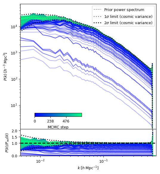
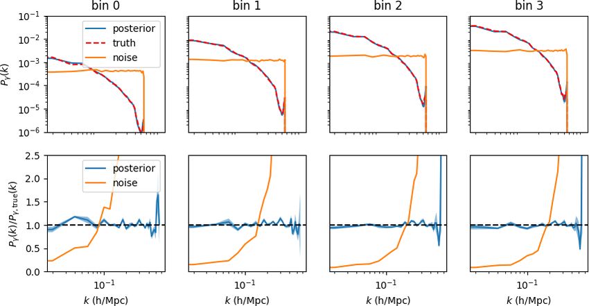
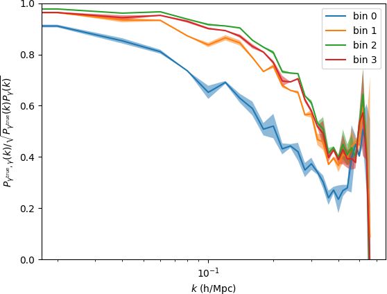
Bayesian forward modelling of cosmic shear 7

Figure 8. Posterior power spectrum of the shear field compared to the power spectrum of the true shear for each tomographic bin. The posterior power spectrum
is the averaged of the power spectrum measured in 500 posterior samples. The orange line shows the noise power spectrum. The bottom plots show the ratio
between the posterior and the true power spectrum, showing that the method recovers the true shear power spectrum at all scales.

 Figure 10. Distribution of the convergence field for tomographic bins cen-
 tred at different redshifts. For comparison, a Gaussian with the same mean
 and variance is plotted on top. The convergence distribution is skewed for
Figure 9. Correlation coefficient between the posterior-predicted and true tomographic bins centered at > 0.5.
shear fields, from 500 posterior samples. This shows the expected Wiener-
filter-like suppression of power where the noise is high.

 is computed from the non-linear density field. Using our forward
knowledge of gravitational physics and, for this reason, we include model, we have computed the convergence field in a wider range of
a gravity model in our Bayesian hierarchical model. The advantage tomographic bins, centred at different redshifts but with the same bin
here is that we sample from the initial field, which we know to be width ( = 0.1), to illustrate more clearly how non-Gaussianity in
Gaussian, so rather than relying on an uninformative prior for the the 1-point distribution evolves. Figure 10 shows the distribution of
final shear fields, we use the correct Gaussian distribution for the these convergence fields. While the convergence shows a Gaussian
initial conditions. What we do not yet do in this model is to vary the distribution for tomographic bins centred at > 0.5, it is skewed for
prior parameters of the power spectrum (as Alsing et al. (2016) do), tomographic bins at lower redshifts. This indicates that the Gaussian
and this will be the subject of future work. As described in section approximation is accurate at large redshift, but it is sub-optimal for
2, we obtained the shear on a flat-sky from the convergence, which low-redshift bins.

 MNRAS 000, 1–11 (2020)

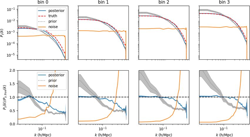
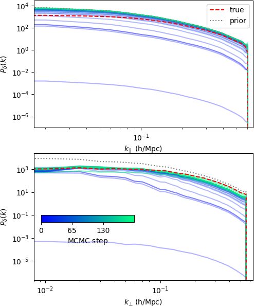
8 N. Porqueres et al.

 Figure 12. Histogram of the shear residuals for the prior test. The residuals
 are computed as the difference between the mean posterior-predicted shear
 and true shear. The distribution of shear residuals is narrower than the noise
 distribution, indicated in green.

Figure 11. Burn-in phase of the dark matter power spectra for the prior test. however, suffices to explain the data, obtaining shear residuals below
We show the power spectrum for the modes parallel to the line-of-sight, k the noise level, as can be seen in Fig. 12. Figure 13 shows the lens-
(upper panel), and the perpendicular modes, ⊥ (lower panel), i.e. in the plane ing power spectrum, indicating that the method recovers the correct
of the sky. The dotted line indicates the prior matter power spectrum, and the lensing power at large scales where the noise is low. However, the
truth is indicated by the red dashed line. The colour scale indicates the sample small scales have lower S/N, and the posterior power spectrum drifts
number in the Markov chain. After the burn-in phase, the method recovers towards the prior. To avoid this prior sensitivity, we need to sample
the correct matter power on the plane of the sky. However, the data is not
 from the power spectrum as well as the field. This will be the subject
constraining in the radial direction and the prior dominates. We note that as
currently implemented, isotropy is not a requirement.
 of a future paper.
 In future work, we will extend our Bayesian hierarchical model to
 jointly sample the cosmological parameters and the density field, us-
 ing an approach compatible with the one presented in Ramanah et al.
7 PRIOR TEST
 (2019). We expect that this future extension of the method will con-
As discussed in section 5.1, in this approach, we keep the cosmology strain the matter power spectrum, also in the radial direction, through
fixed, and specify a prior on the initial power spectrum. Although our the assumption of isotropy, but we do not anticipate being able to
method does not sample the power spectrum, the power spectrum of recover the small-scale radial distribution at the field level, because
the posterior samples is conditioned by the data. This means that, if of the width of the lensing kernel and the distance uncertainties.
the data require it, the posterior power spectrum deviates from the Meanwhile, the test presented here shows that the posterior power
prior, and the density samples have a power spectrum that differs spectrum is conditioned by the data despite using a fixed cosmology.
from the prior. To demonstrate that, we tested our method with mock
data generated with ℎ = 0.6, 8 = 0.55, Ω = 0.7 and analyse these
data with ℎ = 0.677, 8 = 0.8, Ω = 0.3, such that Ω ℎ2 changes
 8 SUMMARY AND DISCUSSION
by a factor 2. These changes in the cosmological parameters give a
different shape and amplitude of the power spectrum, as can be seen We have developed a Bayesian physical forward model to infer the
in Fig. 11. The resolution, total number of sources per square arcmin, matter density field and primordial fluctuations from cosmic shear
the mask and tomographic bins remain as described in Section 4. data. This framework consists of a Gaussian prior for the primordial
 Figure 11 presents the evolution of the power spectrum for this fluctuations, a dynamical structure formation model that links the
test, showing the burn-in phase of the Markov chain. In the plane of initial conditions and the evolved density field, and a likelihood based
the sky, the posterior power spectrum agrees with the truth, demon- on a data model of the cosmic shear in the flat-sky approximation.
strating that the method is sensitive to the true power spectrum even This forward modelling approach allows us to go beyond the com-
when this differs from the prior. However, in the line-of-sight di- mon analyses of cosmic shear based on two-point statistics. While
rection, the data is not constraining, and the prior dominates. These many studies of the cosmic shear focus on the power spectrum or the
results are consistent with Simon et al. (2009). As currently imple- correlation function, the non-linear dynamics of the large-scale struc-
mented, isotropy is not required, and the method cannot determine ture encode significant information in higher-order statistics associ-
the radial power accurately. The recovered matter power spectrum, ated with the filamentary structure of the cosmic web. Our dynamical

MNRAS 000, 1–11 (2020)

Bayesian forward modelling of cosmic shear 9

Figure 13. Posterior power spectrum of the shear field compared to the power spectrum of the true shear for the prior test. The grey dotted line indicates the
shear power spectrum computed using the prior cosmology, which differs from the truth. The orange line indicates the power spectrum of the noise. The bottom
plots show the ratio between the posterior, prior, and noise and the true power spectrum, showing that the method recovers the true lensing power spectrum
where the signal-to-noise is high, but is suppressed in the low S/N regions where the prior is low.

forward model reproduces the filamentary matter distribution and, both the geometry and the power spectrum and its growth. We expect
in this way, allows using every data point, rather than relying on that this extension will also constrain the matter power spectrum in
summary statistics that do not capture all the information and whose the radial direction through the imposition of isotropy, and remove
distributions are not well known. By employing a more accurate the prior power spectrum sensitivity.
gravity model, our method also improves over previous Bayesian To summarise, this work demonstrates the feasibility of detailed
hierarchical approaches that assumed a Gaussian distribution of the and physically plausible inference of the large-scale structure from
shear field (Alsing et al. 2016). cosmic shear data. The proposed approach, therefore, improves the
 We have tested our inference method with simulated data with shear data model from previous methods by including a physical
four tomographic bins, a survey mask, and 30 sources per arcmin2 description of gravity, providing a better representation of the data
as expected for the Euclid survey. These tests demonstrate that our and allowing us to extract information beyond the two-point statistics.
method recovers the unbiased matter distribution and initial matter In future work, we will explore the constraints on cosmology that this
power spectrum from cosmic shear data. Posterior predictive tests approach provides by jointly sampling the initial conditions and the
showed that the inferred quantities are known to the sub-noise level, cosmological parameters.
with additional constraints coming from the cosmological prior.
 Although our framework currently uses a fixed cosmology, we
have shown that the method recovers the true power spectrum when ACKNOWLEDGEMENTS
this differs from the prior where the signal-to-noise is high. While This work was supported by STFC through Imperial College Astro-
we do not sample the power spectrum, the posterior power spectrum physics Consolidated Grant ST/5000372/1. GL acknowledges finan-
deviates from the prior if the data require it. To illustrate this, we cial support from the ANR BIG4, under reference ANR-16-CE23-
performed a test using different values of 0 , 8 and Ω to generate 0002. This work was carried out within the Aquila Consortium1 .
the mock data and to analyse them. In this case, the prior power
spectrum, therefore, differs from the true power spectrum. This test
demonstrated that our method is sensitive to the underlying cosmol-
ogy, and the power spectrum of the density samples is conditioned DATA AVAILABILITY
by the data, recovering the true matter power spectrum across the sky The data underlying this article will be shared on reasonable request
and the lensing power spectrum. However, in the radial direction, the to the corresponding author.
data is not informative, and the prior dominates since we have not
imposed isotropy. In future work, we will extend our Bayesian hier-
archical approach to sample the cosmological parameters, through 1 https://aquila-consortium.org

 MNRAS 000, 1–11 (2020)

10 N. Porqueres et al.
REFERENCES Porqueres N., Jasche J., Lavaux G., Enßlin T., 2019b, A&A, 630, A151
 Porqueres N., Hahn O., Jasche J., Lavaux G., 2020, A&A, 642, A139
Alsing J., Heavens A., Jaffe A. H., Kiessling A., Wandelt B., Hoffmann T.,
 Ramanah D. K., Lavaux G., Jasche J., Wand elt B. D., 2019, A&A, 621, A69
 2016, MNRAS, 455, 4452
 Schneider P., Lombardi M., 2003, A&A, 397, 809
Alsing J., Heavens A., Jaffe A. H., 2017, MNRAS, 466, 3272 Semboloni E., Schrabback T., van Waerbeke L., Vafaei S., Hartlap J., Hilbert
Bernardeau F., van Waerbeke L., Mellier Y., 1997, A&A, 322, 1 S., 2011, MNRAS, 410, 143
Bernardeau F., van Waerbeke L., Mellier Y., 2003, A&A, 397, 405 Simon P., Taylor A. N., Hartlap J., 2009, MNRAS, 399, 48
Böhm V., Hilbert S., Greiner M., Enßlin T. A., 2017, Phys. Rev. D, 96, 123510 Smith K. M., 2006, Phys. Rev. D, 74, 083002
Brown M. L., Castro P. G., Taylor A. N., 2005, MNRAS, 360, 1262 Spergel D., et al., 2015, arXiv e-prints, p. arXiv:1503.03757
Cardone V. F., Camera S., Mainini R., Romano A., Diaferio A., Maoli R., Springel V., 2005, MNRAS, 364, 1105
 Scaramella R., 2013, MNRAS, 430, 2896 Takada M., Jain B., 2003, MNRAS, 344, 857
Chon G., Challinor A., Prunet S., Hivon E., Szapudi I., 2004, MNRAS, 350, Tassev S., Zaldarriaga M., Eisenstein D. J., 2013, J. Cosmology Astropart.
 914 Phys., 2013, 036
Dietrich J. P., Hartlap J., 2010, MNRAS, 402, 1049 Taylor P. L., Kitching T. D., Alsing J., Wandelt B. D., Feeney S. M., McEwen
Eisenstein D. J., Hu W., 1998, ApJ, 496, 605 J. D., 2019, Phys. Rev. D, 100, 023519
Eisenstein D. J., Hu W., 1999, ApJ, 511, 5 Troxel M. A., et al., 2018, Phys. Rev. D, 98, 043528
Euclid Collaboration et al., 2020, A&A, 635, A139 Vafaei S., Lu T., van Waerbeke L., Semboloni E., Heymans C., Pen U.-L.,
Fu L., et al., 2014, MNRAS, 441, 2725 2010, Astroparticle Physics, 32, 340
Gelman A., Carlin J. B., Stern H. S., Rubin D. B., 2004, Bayesian Data van Waerbeke L., Bernardeau F., Mellier Y., 1999, A&A, 342, 15
 Analysis, 2nd ed. edn. Chapman and Hall/CRC van Waerbeke L., et al., 2013, MNRAS, 433, 3373
Gupta A., Matilla J. M. Z., Hsu D., Haiman Z., 2018, Phys. Rev. D, 97,
 103515
Heymans C., et al., 2013, MNRAS, 432, 2433
Hikage C., et al., 2019, PASJ, 71, 43 APPENDIX A: ADJOINT GRADIENT OF THE DATA
Hildebrandt H., et al., 2017, MNRAS, 465, 1454 MODEL
Jain B., Seljak U., 1997, ApJ, 484, 560
Jain B., van Waerbeke L., 2000, ApJ, 530, L1 The inference of the density field requires inferring the amplitudes
Jarvis M., Bernstein G., Jain B., 2004, MNRAS, 352, 338 of the primordial density at different volume elements of a regular
Jasche J., Kitaura F. S., 2010a, MNRAS, 407, 29 grid, commonly between 1283 and 2563 volume elements. This im-
Jasche J., Kitaura F. S., 2010b, MNRAS, 407, 29 plies 106 to 107 free parameters. To explore this high-dimensional
Jasche J., Lavaux G., 2017, A&A, 606, A37 parameter space efficiently, the BORG framework employs a Hamil-
Jasche J., Lavaux G., 2019, A&A, 625, A64
 tonian Monte Carlo (HMC) method, which adapts to the geometry
Jasche J., Wandelt B. D., 2013a, MNRAS, 432, 894
 of the problem by using the information in the gradients. Therefore,
Jasche J., Wandelt B. D., 2013b, MNRAS, 432, 894
Jasche J., Leclercq F., Wandelt B. D., 2015, J. Cosmology Astropart. Phys.,
 this algorithm requires the derivatives of the forward model. In this
 1, 036 appendix, we derive the adjoint gradient of the shear model, which
Jeffrey N., Heavens A. F., Fortio P. D., 2018, Astronomy and Computing, 25, linearly transforms the error vector from the likelihood space to the
 230 parameter space of initial conditions.
Kacprzak T., et al., 2016, MNRAS, 463, 3653 More specifically, the HMC relies on the availability of a gradient
Kayo I., Takada M., Jain B., 2013, MNRAS, 429, 344 of the posterior distribution. Therefore, we need to compute the gra-
Kilbinger M., 2015, Reports on Progress in Physics, 78, 086901 dient of the log-likelihood with respect to the initial density contrast,
Kitching T. D., Heavens A. F., Miller L., 2011, MNRAS, 413, 2923 ic .
Kitching T. D., et al., 2014, MNRAS, 442, 1326
Kitching T. D., Heavens A. F., Das S., 2015, MNRAS, 449, 2205
 log L ∑︁ ∑︁ log L 
Kitching T. D., Verde L., Heavens A. F., Jimenez R., 2016, MNRAS, 459, 
 = (A1)
 971 ic
 
 ic
 
LSST Science Collaboration et al., 2009, arXiv e-prints, p. arXiv:0912.0201
Laureijs R., et al., 2011, arXiv e-prints, p. arXiv:1110.3193
 
 ∑︁ ∑︁ ˆ 1, 
 − 1, 
Lavaux G., Jasche J., 2016, MNRAS, 455, 3169 log L 1, 
Lavaux G., Jasche J., Leclercq F., 2019, arXiv e-prints, p. arXiv:1909.06396 = 2
 (A2)
Leclercq F., Faure B., Lavaux G., Wandelt B. D., Jaffe A. H., Heavens A. F.,
 ic
 ic
 
 Percival W. J., 2020, A&A, 639, A91 
 ˆ 2, 
 − 2, 
 2, 
Lin C.-A., Kilbinger M., 2015, A&A, 583, A70 + 2
Liu J., Petri A., Haiman Z., Hui L., Kratochvil J. M., May M., 2015a, Phys. ic
 
 Rev. D, 91, 063507
Liu X., et al., 2015b, MNRAS, 450, 2888 " 2
 − 2 
 !#
 log L ∑︁ ∑︁ ˆ 1, − 1, 
Marian L., Smith R. E., Hilbert S., Schneider P., 2012, MNRAS, 423, 1711 = DFT −1
 DFT
Maturi M., Fedeli C., Moscardini L., 2011, MNRAS, 416, 2527 ic 2
 2 + 2 ic
 
Peel A., Lin C.-A., Lanusse F., Leonard A., Starck J.-L., Kilbinger M., 2017, " !#
 
 ∑︁ ∑︁ ˆ 2, 
 − 2, 
 A&A, 599, A79 −1 −2 
Pen U.-L., Zhang T., van Waerbeke L., Mellier Y., Zhang P., Dubinski J., + 2
 DFT DFT
 2 + 2 ic
 
 2003, ApJ, 592, 664
Petri A., Haiman Z., Hui L., May M., Kratochvil J. M., 2013, Phys. Rev. D, with
 88, 123002
Pires S., Leonard A., Starck J.-L., 2012, MNRAS, 423, 983 3 02 Ω h ∑︁
 2
 ( − ) i Δ M ( , ic )
Planck Collaboration 2019, arXiv e-prints, p. arXiv:1905.05697
 = ( )Δ 
 ic
 2 2 = 
 ic
 
Porqueres N., Kodi Ramanah D., Jasche J., Lavaux G., 2019a, A&A, 624,
 A115 (A3)

MNRAS 000, 1–11 (2020)

Bayesian forward modelling of cosmic shear 11
where M ( , ic ) is the dynamical forward model.

This paper has been typeset from a TEX/LATEX file prepared by the author.

 MNRAS 000, 1–11 (2020)