Modeling and Parameter Identification of MR Damper considering Excitation Characteristics and Current

Hindawi
Shock and Vibration
Volume 2021, Article ID 6691650, 17 pages
https://doi.org/10.1155/2021/6691650

Research Article
Modeling and Parameter Identification of MR
Damper considering Excitation Characteristics and Current

 Shuguang Zhang, Wenku Shi, and Zhiyong Chen
 State Key of Automobile Simulation and Control Laboratory, Jilin University, Changchun 130022, China

 Correspondence should be addressed to Zhiyong Chen; chen_zy@jlu.edu.cn

 Received 28 December 2020; Revised 22 January 2021; Accepted 25 March 2021; Published 8 April 2021

 Academic Editor: Giosuè Boscato

 Copyright © 2021 Shuguang Zhang et al. This is an open access article distributed under the Creative Commons Attribution
 License, which permits unrestricted use, distribution, and reproduction in any medium, provided the original work is
 properly cited.
 Smart structures such as damping adjustable dampers made of magnetorheological (MR) fluid can be used to attenuate vibration
 transmission in vehicle seat suspension. The main research content of this paper is the nonlinearity and hysteresis characteristics
 of the MR damper. A hysteretic model considering both excitation characteristics and input current is proposed to fit the damper
 force-velocity curve for the MR damper under different conditions. Multifactor sensitivity analysis based on the neural network
 method is used to obtain importance parameters of the hyperbolic tangent model. In order to demonstrate the fitting precision of
 the different models, the shuffled frog-leaping algorithm (SFLA) is employed to identify the parameters of MR damper models.
 The research results indicate that the modified model can not only describe the nonlinear hysteretic behavior of the MR damper
 more accurately in fixed conditions, compared with the original model, but also meet the fitting precision under a wide range of
 magnitudes of control current and excitation conditions (frequency and amplitude). The method of parameter sensitivity analysis
 and identification can also be used to modify other nonlinear dynamic models.

1. Introduction The structure of the magnetorheological damper is
 similar to the structure of an ordinary vehicle cylinder
Vehicle ride comfort plays an important role in vehicle damper. The medium inside the MR damper is a magne-
dynamics research, in which the transmission of vibration torheological fluid. The MR fluid can reversibly change from
through seat exerts a crucial influence. Traditional passive free flowing, linear viscous liquids to non-Newtonian fluid
seat suspensions are very limited in terms of ride comfort with a controllable yield strength when exposed to a mag-
and cannot meet the increasingly stringent comfort re- netic field [13].
quirements. In recent years, the semiactive seat suspension However, the magnitude of the generated damper force
system is becoming more and more popular due to simple is related to many factors that involve many nonlinear el-
structure, low power consumption, good vibration damping ements and increase model complexity of the MR damper.
behavior, and high reliability [1–6]. The causes of nonlinearity are listed as follows: (1) different
 There are many types of semiactive suspensions such as magnetoresistivity of electromagnetic circuits; (2) hydro-
throttle variable damper suspension, air suspension, elec- dynamics of MR fluid flowing in piston gap; (3) the chemical
trorheological damper suspension, and magnetorheological properties of MR fluid; and (4) the relationship between the
damper suspension [7, 8]. Therefore, an MR damper is a yield stress generated by MR fluid and applied magnetic field
fluid damping device, widely used in vibration control of strength.
civil engineering structures and mechanical systems because Various papers have established MR damper mechanical
of its wide damping adjustable range, short adjustment time, models by various proposed methods. According to relevant
high reliability, and low cost [9–12]. literature, MR damper force models are divided into three

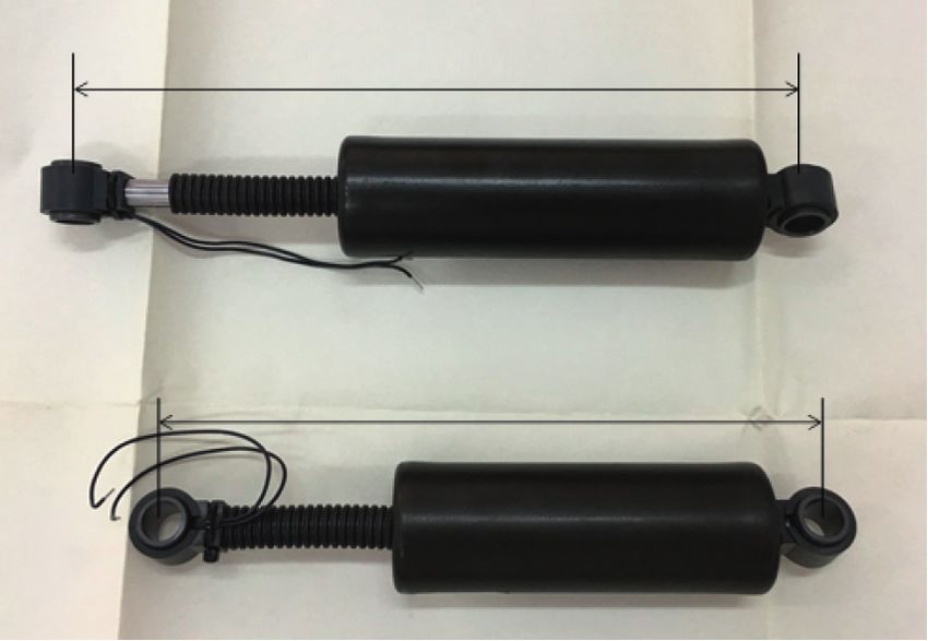
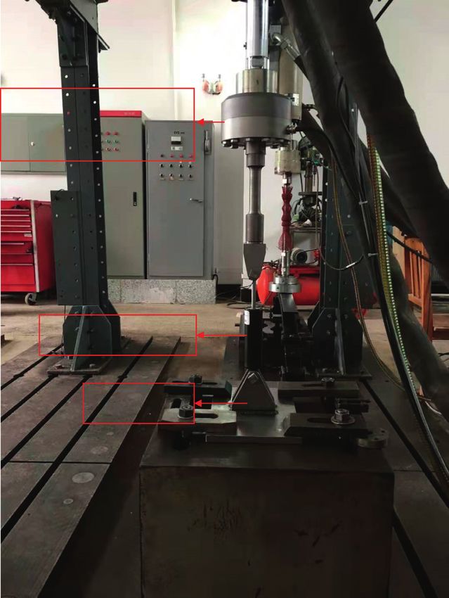
2 Shock and Vibration

main groups [10, 14–16]: pseudostatic models, parametric
models, and nonparametric models. In pseudostatic models, 248 mm
the damper force is calculated by the pressure difference
between the two ends of the damper piston, structural pa-
rameters, MR fluid parameters, and magnetic field strength
[17]. This type of model can generally reflect the force-
displacement characteristics properly, but the fitting of the
force-velocity characteristics is not accurate enough. Pseu- 208 mm
dostatic models are mainly used for the design of MR
dampers, but not suitable for the research of semiactive
suspension control. Parametric models and nonparametric
models are mainly distinguished according to whether the
parameters make sense in physical. Nonparametric models
generally consider that the damper force consists of a Figure 1: Picture of the MR damper.
polynomial with input current and damper velocity, or
neural network model [18]. And, in parametric models, the 8040-1), respectively. Except the length of stroke, the two
damper force is calculated by physically meaningful pa- dampers have the same structure parameters and MR fluid.
rameters. There are many types of parametric models, The damper consists of two liquid chambers that are sep-
among which the Bingham model is the most basic one. arated by a piston with small orifices. The rated value of the
Although this model can describe the relationship between input current is 1 A in the electromagnet coil around the
the damper force and displacement well, it cannot reflect the piston head.
hysteresis relationship of force-velocity. At present, the Figure 2 shows the experimental setup including actu-
Bouc–Wen model is widely used, which can exactly describe ator, computer closed-loop control electro-hydraulic servo
the hysteretic characteristics of the MR damper force versus system, force sensor, displacement sensor, fixture, and
piston velocity by designing the hysteresis variable z. constant current power supply. The damper was driven by a
However, the nonlinear differential equations contained in Schenck actuator, and the position sensor and force
the Bouc–Wen model inevitably increases difficulty to pa- transducer were used to collect the measured displacement
rameter identification. In 1997, Spencer and Dyke [19] and damper force of the two dampers.
proposed a modified Bouc–Wen model, which further Sine vibrations, with the frequency range from 0.5 Hz to
improved the fitting accuracy of the force-velocity hysteresis 9 Hz and vibration amplitude of 5 mm, 10 mm, 15 mm, and
curve. There is a wide range of parametric models: nonlinear 20 mm, were provided by the actuator. And, the current
hysteretic biviscous model, generalized sigmoid hysteresis inputs ranged from 0 to 1 A with 0.2 A intervals. The
model, hyperbolic tangent function-based model, and so on. specification of excitations is shown in Table 1.
However, the previous models have shortcomings in terms
of model accuracy, complexity, or limitation [14, 16, 20–22].
 The purpose of this paper is to build a detailed model of 2.2. Experimental Results. In the following analysis, only the
the MR damper used for semiactive suspension control. The results of the RD-8040-1 damper were discussed, in which
paper is structured as follows: in Section 2, the mechanical the mechanical behaviors of the two dampers were similar,
performance test of the MR damper was performed to study as was shown in the experiment. The responses of the MR
the characteristics of damper force in different excitation damper applied a 20 mm 2 Hz sinusoid excitation which are
inputs. In Section 3, several classic MR damper models were shown in Figure 3, at six constant current values, 0 A, 0.2 A,
introduced in detail, and the more suitable model was se- 0.4 A, 0.6 A, 0.8 A, and 1 A. Figures 3(a) and 3(b) illustrate
lected. In Section 4, the sensitivity analysis method of pa- the force-displacement (f-d) and the force-velocity (f-v)
rameters of the hyperbolic tangent model was applied to characteristics, respectively. It is obvious that the f-d curve is
illustrate the importance of every model parameter, as approximately rounded rectangle. There are evident bumps
references for model extensions in subsequent chapters. The near the zero-displacement area, which is caused by the
shuffled frog-leaping algorithm used for parameter identi- elasticity of the damper. The effect of changing current value
fication is explained in Section 5. Subsequently, the iden- is readily observed, and the damper force curve rises
tification results of damper hysteretic model parameters are monotonically as the current value increases. The increase of
discussed and an extended hysteresis model is achieved and current value is found to be nonlinear in nature. Under
verified in Section 6. In the end, conclusions are presented in 20 mm 2 Hz sinusoid excitation, the maximum damper force
Section 7. increases by 450.71N when current value increases from
 0.2 A to 0.4 A. Similarly, for increase from 0.4 A to 0.6 A and
2. Experimental Study of the MR Damper from 0.6 A to 0.8 A, the maximum damper force increases by
 297.02 N and 324.06 N severally. When the current value
2.1. Experimental Setup. Two types of MR dampers, shown increases from 0.8 A to 1 A, the increment of maximum
in Figure 1, were employed for dynamic tests in this study. damping force is 64.52N. It can be also observed that the
The strokes of the pistons of these two dampers are 74 mm magnetic field intensity generated by the electromagnetic
(long stroke, RD-8041-1) and 55 mm (short stroke, RD- coil is close to the magnetic saturation intensity once the

Shock and Vibration 3

 increasing frequency, keeping the current and amplitude
 invariable. As the frequency grows higher, the area enclosed
 by the damper force-displacement loops increases, and the
 energy dissipation in each vibration cycling increases. As is
 Actuators with shown in Figure 4(b), the damper force at the same velocity
 built-in sensors is approximately equal and shows the Bingham plastic be-
 havior of the MR damper when the velocity and acceleration
 are in the same direction. However, the damper force in the
 same velocity decreases when frequency grows higher, in
 case the velocity and acceleration are reversed. This phe-
 nomenon of the MR damper is because the MR fluid
 presents viscoelasticity at low velocity and viscoplasticity at a
 high velocity. Furthermore, the size of the hysteresis loop
 MR damper
 mainly depends on the inertia effect of damper. The area of
 hysteresis loops increases due to the large inertia resulting
 Fixtures from the high acceleration as the velocity direction changes.
 In Figures 5(a) and 5(b), the area enclosed by the damper
 force-displacement curve increases as the excitation am-
 plitude increases under the same input current and fre-
 quency, and the area of force-velocity hysteresis loop
 becomes larger as well.
 Based on the characterizations of the MR damper above,
 it can be observed that the MR damper behaves strong
 nonlinearity. All of the excitation amplitudes, frequencies,
 Figure 2: Experimental setup. and input currents have impacts on the mechanical char-
 acteristics of the MR damper.
 It is difficult to accurately describe the MR damper
 Table 1: Specification of excitation.
 model by conventional methods. The establishment of a
 Amplitude in (mm) comprehensive dynamic model of the MR damper has an
Frequency 5 10 15 20 important influence on the control of the semiactive seat
0.5 Hz √ √ √ √ suspension system. In this study, a detailed hysteretic model
1 Hz √ √ √ √ was established to describe the mechanical characteristics of
1.5 Hz √ √ √ √ the MR damper for the purpose of vehicle suspension
2 Hz √ √ √ √ control.
2.5 Hz √ √ √ √
3 Hz √ √ √ √
3.5 Hz √ √ √ √ 3. The Mechanical Models of the MR Damper
4 Hz √ √ √ √
4.5 Hz √ √ √ — As a controllable fluid, MR fluid is a Newtonian fluid that
5 Hz √ √ √ — can freely flow in the initial state and turns into non-
6 Hz √ √ — — Newtonian fluid when exposed to a magnetic field. The
7 Hz √ √ — —
 change of MR fluid viscous is reversible and reflected by a
9 Hz √ — —
 significant variation in the damper output force.
 A lot of models have been proposed to describe the
current value increases above 0.8 A, reflected in which the nonlinear behavior of the damper force versus velocity of
increment of the damper force of the MR damper becomes MR dampers. There are a couple of models that were
smaller. commonly employed in the previous work such as the
 The damper force-velocity curve is symmetrical and Bingham model, Bouc–Wen model, nonlinear hysteretic
nonlinear, with apparent hysteresis characteristics. When biviscous model, generalized sigmoid hysteresis model,
the velocity of the piston increases, the damper force in- hyperbolic tangent function-based model, and so on
creases along the lower branch curve. The hysteresis curve of [23–29].
damper force moves counterclockwise with damper velocity. Bouc–Wen model is widely used in the modeling of
When the input current value of the coil increases, the hysteretic systems (Figure 6). It can exhibit various hys-
hysteresis loop of the damper force-velocity of the MR teretic behaviors by changing its model parameters and has
damper gradually increases. very good adaptability. The expression is shown as follows:
 Figure 4(a) shows the force-displacement characteristics
with 0.8 A current applied under 5 mm sine vibration and F � c0 x_ + k0 x − x0 + αz,
various frequency (1 Hz, 2 Hz, 3 Hz, 4 Hz, 5 Hz, 6 Hz). It can n− 1
 (1)
 z_ � −c|x|z|z|
 _ _ n + Ax,
 − βx|z| _
be observed that the maximum damper force increases when

4 Shock and Vibration

 2000 2000

 1500 1500

 1000 1000
 Damper force (N)

 Damper force (N)
 500 500

 0 0

 –500 –500

 –1000 –1000

 –1500 –1500

 –2000 –2000
 –25 –20 –15 –10 –5 0 5 10 15 20 25 –300 –200 –100 0 100 200 300
 Displacement (mm) Velocity (mm/s)

 0A 0.6 A 0A 0.6A
 0.2A 0.8 A 0.2 A 0.8A
 0.4A 1A 0.4 A 1A
 (a) (b)

Figure 3: Mechanical properties of different currents, frequency � 2 Hz, and amplitude � 20 mm. (a) Damper force-displacement.
(b) Damper force-velocity.

 1500 1500

 1000 1000

 500 500
 Damper force (N)

 Damper force (N)

 0 0

 –500 –500

 –1000 –1000

 –1500 –1500
 –7 –5 –3 –1 1 3 5 7 –220 –160 –100 –40 20 80 140 200
 Displacement (mm) Velocity (mm/s)
 1Hz 4Hz 1 Hz 4 Hz
 2Hz 5Hz 2 Hz 5 Hz
 3Hz 6Hz 3 Hz 6 Hz
 (a) (b)

Figure 4: Mechanical properties of different frequencies, current � 0.8 A, and amplitude � 5 mm. (a) Damper force-displacement.
(b) Damper force-velocity.

where, α, β, c, and n are the model parameters and z is a model. But, in the low-speed area, the model is not accurate
hysteresis variable. The bias force generated by the accu- enough to fit the velocity hysteresis characteristics.
mulator inside the MR damper is converted to the initial Spencer proposed a modified Bouc–Wen model in order
offset x0 of the spring k0. The Bouc–Wen model has good to more exactly predict the damper response in low velocity.
fitting accuracy for the damper force-velocity characteristics The damper force is given as
of MR dampers. However, it makes great difficulty to the
 c0 y_ � αz + k1 x − xin + c1 x_ − x_ in ,
parameter identification and may affect the robustness of the 
 _
control system, due to the existence of the differential term z. z_ � −c x_ − x_ in z|z|n− 1 − β x_ − x_ in |z|n + A x_ − x_ in ,
 Research shows that the Bouc–Wen model can better
 F � c0 x_ in + k0 x − x0 ,
predict the force-displacement and force-velocity charac-
teristics of MR dampers, compared with the Bingham (2)

Shock and Vibration 5

 1700 1700

 1200 1200

 700 700
 Damper force (N)

 Damper force (N)
 200 200

 –300 –300

 –800 –800

 –1300 –1300

 –1800 –1800
 –22 –18 –14 –10 –6 –2 2 6 10 14 18 22 –280–230–180–130 –80 –30 20 70 120 170 220 270
 Displacement (mm) Displacement (mm)
 5 mm 15mm 5 mm 15mm
 10mm 20mm 10 mm 20mm
 (a) (b)

Figure 5: Mechanical properties of different amplitudes, current � 0.8 A, and frequency � 2 Hz. (a) Damper force-displacement. (b)
Damper force-velocity.

 Bouc–Wen x xin
 Bouc–Wen
 x

 c1
 k0
 k0
 F F
 c0

 c0
 k1

 Figure 6: Bouc–Wen model.
 Figure 7: Modified Bouc–Wen model.

where c0 and c1 represent the viscous damping at low ve- x
 Hysteresis
locity and high velocity, respectively; k1 represents stiffness
at high speed; and xin is the internal variate of displacement,
as shown in Figure 7. Other parameters are consistent with
the Bouc–Wen model. Although the accuracy of the model is k0
improved, the complexity of the model also increases sig- F
nificantly. The newly brought differential intermediate
variable in this model brings greater challenges in parameter C0
identification and the robustness of control system.
 Kwok and Ha [30] proposed a damper model in 2006.
They used a hyperbolic tangent function to represent the Figure 8: Hyperbolic tangent model.
hysteresis element z (see Figure 8). The viscosity and stiffness
elements are expressed by linear functions c0 x_ and k0 x. Due
to lack of differential equations, the calculation efficiency of shows the comparison of the calculation results of the two
this model is promoted, and parameter identification be- models. The fitting accuracy of the hyperbolic tangent model
comes simple to operate. The model is expressed as follows: is higher than the Bouc–Wen model especially in the velocity
 transition zone. The output damping force error RMS of the
 z � tanh(βx_ + δsign(x)), two models compared to the test damping force are 30.88N
 (3) and 49.49N, respectively.
 F � c0 x_ + k0 x + αz + F0 .
 By comparing different hysteretic models, it can be
 Through calculation and analysis, it can be found that the found that the hyperbolic tangent model is simple in
hyperbolic tangent model can accurately fit the velocity- structure and does not contain differential terms. Mean-
damping force hysteresis curve of the MR dampers. Figure 9 while, it can fit the velocity-damping force hysteretic

6 Shock and Vibration

 750 parameters on the accuracy of the model. Furthermore, in
 subsequent model extensions, model design was based on
 450 the ranking of parameter sensitivity, focusing on parameters
 Damper force (N)

 150 with larger sensitivity coefficients, and establishing the re-
 lationships between model parameters and excitation
 –150 characteristics or input current. In this way, the number of
 model parameters is minimized as much as possible on the
 –450
 premise of ensuring model accuracy. Therefore, the com-
 –750 plexity of the model is reduced, and the computational
 efficiency of the model is improved.
 –1050
 –260 –160 –60 40 140 240 There are plenty of sensitivity techniques in previous
 Velocity (m/s) research, and the results of sensitivity ranking may exist
 slightly disparity for different methods [32]. In this paper,
 Experimental data
 Hyperbolic tangent model
 multiparameter sensitivity analysis based on BP neural
 Bouc–Wen model network was put in use.
 The neural network (NN) models are well known for
 Figure 9: The calculation results of different models. strong self-learning adaptability, high robustness, and ex-
 cellent fault tolerance. It can reflect the implicit feature rules
characteristics of the MR damper precisely. Therefore, the by the connection weights between neurons and solve many
hyperbolic tangent model is selected for extended research nonlinear problems including complex information, unclear
in this paper. rules, and noise pollution. The neural network models can
 evaluate the sensitivity values of model parameters in the
4. Parameter Sensitivity Analysis situation that multiple parameters change simultaneously in
 complex models [33].
Sensitivity analysis of the mathematical model parameters is In this paper, the BP neural network was employed to
not only critical to model validation but also can provide quantify the sensitivity of parameters of the damper force
guidance for research of parameters analysis. The analysis of model. The weights and thresholds of the input layer to the
hyperbolic tangent hysteresis model shows that it can predict hidden layer and of the hidden layer to the output layer were
response for fixed current input and vibration excitation. extracted through training the BP neural network with
However, the model parameters under different currents sample database. The BP neural network model and weights
and excitation conditions are different. In order to establish represented the mapping relationship between each pa-
a general model suitable for different working conditions, a rameter and output. The method of Garson (equation (5))
hysteresis model including current, amplitude, and fre- was applied to compute the sensitivity values of model
quency characteristics is needed. The method of sensitivity parameters.
analysis can distinguish the important parameters from 
 m n 
unimportant parameters in the mathematical model [31]. j�1 wij wjk / i�1 wij 
Due to the large number of parameters in the hyperbolic RI � , (5)
 ni�1 m w w / n w 
tangent model, the sensitivity analysis about the contribu- j�1 ij jk i�1 ij 
tion of the parameters to the MR damper model output is
carried out to filter out the parameters with poor sensitivity. where Wij � the connection weight from input unit to hidden
The relationships between the sensitive parameters and the unit and Wjk � the connection weight of hidden unit to
excitation characteristics or input current are established, so output unit. The sine excitation at amplitude 10 mm and
as to obtain the extensional MR damper model that is frequency 4 Hz and input current 0.8 A were loaded on the
suitable for different excitation conditions. MR damper to analyse parameters sensitivity.
 In sensitivity analysis, the sensitivity coefficient can be The main steps of sensitivity analysis method based on
expressed as follows: BP neural network are as follows:
 0.5 Step 1. Structure design of neural network: a three-layer
 1⎣N 2
 S� ⎡ F′ − Fi ⎤⎦ , (4) neural network was created, including input layer,
 N i�1 i hidden layer, and output layer, to calculate the sensi-
 tivity values of each model parameter. There are six
where Fi and F′irepresent the model output force values at units in input layer: α, β, δ, F0, c0, and k0, respectively.
the ith sampling spot of parameters before and after The sensitivity values of parameters were calculated by
changing; N � total number of sampling spot; and equation (4). The number of units in the hidden layer
S � sensitivity of parameters. The sensitivity of the parameter was calculated by equation (6)
increases as the value of S becomes larger. √�����
 The main parameters that have relatively significant n1 � n + m + a. (6)
influence on the sensitivity coefficient of damper force were
obtained via adjusting each parameter within its allowable where, n, n1, and m represent separately the number of
range, so as to study the degree of influence of these input unit, hidden unit, and output unit; a � any

Shock and Vibration 7

 constant between 1 and 10. After calculation, the Input layer Hidden layer Output layer
 number of units in the hidden layer was determined to
 be 10. The structure of neural network is illustrated in
 α
 Figure 10.
 Step 2. Selection of training samples for neural network:
 β
 six model parameters, α, β, δ, F0, c0, and k0, were se-
 lected as the training data, whose basic values,
 α � 1025.79, β � 0.01843, δ � 0.9715, F0 � −104.55N, δ
 c0 � 1.83, and k0 � 0.0025, were calculated under 10 mm, S
 4 Hz, and 0.8 A excitation condition. And, five levels for F0
 each parameter, 0, ±30%, and ±50% varied from basic
 values. By combination, 15625 (56) samples were ob- c0
 tained. Therfore, 15,000 samples were selected ran-
 domly as training data, and 625 samples from the k0
 remaining samples were picked out to verify the trained
 neural network model.
 Step 3. Analysis of the neural network model: by Figure 10: The neural network structure.
 analysing the calculation results of the neural network,
 conclusions can be made that there are more than 90%
 samples whose errors are within 5%. Obviously, the complex function optimization problems. Figure 11 shows
 mapping established through the neural network can the parameter identification process of the model.
 get accurate relationship between model parameters Although there are some resemblances between SFLA
 and damper force output. The weights (Wij and Wjk ) and genetic algorithm (both are updated iteratively through
 are listed in Table 2. fitness sorting), the SLFA has a faster spread speed. Memes
 in SFLA can flexibly use different mechanisms to spread
 Table 3 lists the sensitivity coefficients of each model information from one member of the memeplex to another,
parameter calculated by the methods of Garson (equation while genes in GA can only pass from parents to offspring.
(14)). It is noteworthy that the parameter a has the greatest The evolution in genetic algorithm is limited by the number
impact on the damper force output, with the sensitivity value of offspring that a single parent can produce.
of 39.43%. And, β, c0, and d rank behind, with values of Steps of the shuffled frog-leaping algorithm are as
30.68%, 14.76%, and 14.71%, respectively. The remaining follows:
two parameters have only slight effect on the damper force
 Step 1. Initialize parameters and population: set t � 1;
output.
 determine the population size F and randomly generate
 The calculation result of sensitivity analysis show that the
 the initial population X (t); determine the number of
effects of parameter α, β, δ, and c on the model output are
 subpopulations m and the number of individuals in
significant ones; meanwhile, the parameters F0 and k0 can be
 each subpopulation n; F � m ∗ n.
set to constants due to the low sensitivity.
 Step 2. Rank frogs: calculate the fitness values of each
5. The Shuffled Frog-Leaping Algorithm (SFLA) individual frog in the current population X (t).
 Step 3. Partial update iteration: t � t + 1. Sort the entire
To describe the force-velocity hysteretic characteristics of the frog group according to their fitness and perform a
MR damper, the parameters in the MHT model need to be local search in each subpopulation to update the worst
identified. frog.
 Parameter identification is a key issue in this research
due to the complexity and nonlinearity of the model. In (1) During the inner-group update process of the
order to accurately determine the parameters, researchers subpopulation, the algorithm only adjusts the worst
have successively proposed a series of identification methods frog’s position by computing
aimed at nonlinear models, such as genetic algorithm (GA), SW � MIN INT rand FPB − FPW , SWmax ,
particle filter algorithm (PA), and least square method (LSC)
[34]. for positive step
 In this study, the processes of parameter identification � MAX INT rand FPB − FPW , −SWmax ,
utilizing shuffled frog-leaping algorithm and the experiment
 for negative step
data fitting were carried out [35, 36]. The shuffled frog-
leaping algorithm was firstly proposed in 2003 by Lansey and NL � Lw + SW.
Eusuff [37] to solve the combinatorial optimization problem. (7)
This algorithm combines the advantages of particle swarm
algorithm and memetic algorithm and is a new meta- where SW and NL are the regeneration step size
heuristic group evolution algorithm. It has been successfully and the updated position of the worst frog, re-
applied in many fields especially in solving multiobjective spectively; SWmax � the maximum step size of frog

8 Shock and Vibration

 Table 2: The weight of each neuron.
 Wij Wjk
1 0.763677 0.773383 −0.32296 −0.00167 0.30149 1.02E−05 −0.0150
2 1.283121 0.219759 0.129862 −0.02544 0.205786 −0.00162 1.2876
3 −0.7358 −0.14136 0.100185 −1.36419 −0.20055 −0.00179 −0.2472
4 0.934392 −0.144 −0.13751 −0.02174 0.576572 0.001714 0.2388
5 −4.48097 −0.57274 −0.00747 −0.0086 −1.42884 0.002235 −0.1046
6 −0.16682 1.768808 −0.8945 −0.0096 0.29989 −0.00044 2.0922
7 1.833262 −0.5778 −0.07458 −0.0066 0.476606 −0.00023 −47.6325
8 −0.82338 −0.69084 0.310103 0.000858 −0.30901 8.14E−05 49.2800
9 0.869601 −0.31437 0.343672 0.009563 0.28554 0.000773 −8.8736
10 −0.22652 −1.612 1.686386 0.019954 −0.19215 0.009069 0.1586

Table 3: The sensitivity results from the neural network model. influenced by the characteristics of the excitation (amplitude
 and frequency) according to the research in previous sec-
Parameter A β δ tions. The identified parameters extracted from a fixed
Sensitivity (%) 39.4325 30.6834 14.71123 working condition cannot accurately fit for other excitation
Parameter F0 c0 k0 conditions. A general model that is suitable for different
Sensitivity (%) 0.3947 14.7600 0.0180 excitation conditions should be built by establishing the
 relationship between model parameters and loading con-
 movement specifically; FPB � the best solution in ditions including input current, vibration frequency, and
 perform; FPw � the worst solution in amplitude.
 subpopulation. Although several studies have made effort to introduce
 If the calculation results in step 3(1) meet the it- the applied load to the damper model, most of these papers
 eration requirements, move to the step 4; Other- only study the influence of input current on the model
 wise, go to step 3(2). output, without considering excitation characteristics [38].
 (2) Replace FPB in equation (7) with the global optimal Cheng and Chen [39] proposed a model containing am-
 value FPXbest as follows: plitude and frequency.
 Noteworthy, the amplitude and frequency of vibration
 SW � MIN INT rand FPbest − FPW , SWmax , excitations cannot be measured in real time, especially
 for positive step under random excitation. Therefore, it is necessary to
 explore the relationship between excitation characteristics
 � MAX INT rand FPbest − FPW , −SWmax ,
 and measurable parameters during modeling. Wang and
 for negative step Ma [21] proposed a relational expression between move-
 NL � Lw + SW. ment states (displacement, velocity, and acceleration) of an
 MR damper and excitation characteristics. The maximum
 (8) velocity (vm ) of the damper has a linear relationship with
 (3) If the two substeps above cannot meet the iteration the sine excitation amplitude and frequency. vm can thus be
 requirements, the frog that is in the worst position expressed by
 in the subpopulation will jump to a random po- vm � c0 ∗ (a · f), (10)
 sition (rp) in the solution space.
 NL � rp. (9) where c0 is a constant coefficient and a and f represent the
 amplitude and frequency, respectively.
 To verify the equation, the maximum velocity values
 Step 4. The iteration ends after all the subpopulations under a series of working conditions were sorted out and
 have completed the partial search. Mix all the frogs then observed the relationship between the vm and ampli-
 together and regroup according to the updated fitness tude or frequency (see Figure 12). It is evident that the vm
 value. amplitude curve and vm frequency curve both show linear
 Step 5. Determine whether the current result meets the relationships. As for vm variation under fixed amplitude
 convergence demand. If not, go to step 2 and resort and (5 mm, 10 mm, 15 mm, and 20 mm), it increases with the
 divide the memeplex to perform the local search increase of frequency straightly. Similarly, the linear increase
 process. If it does, the process of algorithm ends. relationship of vm versus amplitude is observed under each
 fixed frequency (1–5 Hz). Figure 13 demonstrates that the
6. Parameter Identification and value of vm does not depend on the input of current ap-
 Model Validation proximately under each constant amplitude and frequency.
 Because the variable vm cannot be directly measured in
6.1. Parameter Identification. The dynamic performance of real time either, and the damper instantaneous displacement
the MR damper is not only related to input current but also and acceleration are connected with vm as follows:

Shock and Vibration 9

 Start

 Generate initial sets

 Calculate the fitness of each individuals and rank
 them in descending order of fitness
 Remix all frog individuals

 Y
 The optimal solution Xg
 satisfies the convergence
 Satisfy the number of
 requirement
 Y N iterations of the
 subpopulation N
 Output global
 optimal solution Local searches are performed
 Partition subpopulations
 on subpopulations
 End

 (a)
 for i = 1 to F do % Sort frog individuals by fitness value
 [J_new, index] = sort (J, ‵descend′)
 x = x (index)
 end for
 for i = 1 to m do % Divide the 1st to mth frogs into 1st to mth frog subgroups
 M (1, i) = x (i);
 end for
 u = randperm (F-m); % Randomly shuffle the order of the remaining F-m frogs
 x_randperm = x (m + 1 : F);
 x_randperm = x_randperm (u);
 length = (F-m)/m;
 for j = 1 to length to F-m do % Divided the remaining F-m frogs evenly into m parts
 and randomly assign them to m frog subgroups

 M (1, 2: length + 1) = x_randperm (( j-1) length + 1 : j∗length)
 end for
 (b)

 Figure 11: The algorithm process of SFLA. (a) The flowchart of SFLA. (b) Algorithm steps.

 600
 500
 Vm (mm/s)

 400
 300
 200
 100
 0
 20
 6
 Am 15 5
 plit 4
 ude 10 3 )
 5 2
 (mm
 ) 1 enc y (Hz
 0 0 Frequ
 Figure 12: The relationship between maximum velocity and excitation characteristic.

10 Shock and Vibration

 600

 500

 400

 vm (mm/s)
 300

 200

 100

 0
 5mm–1Hz

 5 mm–2Hz

 5 mm–3Hz

 5 mm–4Hz

 5 mm–5Hz

 10mm–1Hz

 10mm–2Hz

 10mm–3Hz

 10mm–4Hz

 10mm–5Hz

 15mm–1Hz

 15mm–2Hz

 15mm–3Hz

 15mm–4Hz

 15mm–5Hz
 Excitation characteristics
 0A 0.6 A
 0.2A 0.8 A
 0.4A 1A
 Figure 13: The effect of current on maximum velocity under different excitations.

 ��������
 2 vm . For fixed vibration input (vm ), the parameter δ increases
 vm � x_ − x · x, (11)
 as the control current increases. A first-order polynomial can
 approximate the relationship between δ and current precisely.
where x_ is the velocity of the damper andx€ and x represent
instantaneous displacement and acceleration, respectively. δ � δ1 I + δ2 . (14)
Therefore, the excitation frequency and amplitude are
expressed by measurable dynamics variables of the damper Observations from Figures 16(c) and 16(d) are that the
(when the vehicle is operating in real time) by taking ad- parameter c0 linearly rises as current increases, while the
vantage of equations (10) and (11). effect of vm on parameter c0 can be neglected. The parameter
 Here, we firstly identified the parameters of the damper c0 is obtained as follows:
model from experiment data under a wide range of exciting
conditions. The shuffled frog-leaping algorithm was utilized c0 � c01 I + c02 . (15)
to obtain the accurate model parameters. And then, the
 The variations of other parameters, k and F0, have
correlation rules between each parameter and the excitation
 nothing to do with the input current and excitation char-
characteristics (current and vm ) were excavated in purpose
 acteristics (Figure 17), and the sensitivity values of these
of building the general damper model.
 parameters to the model output are quite low without ex-
 The relationships between parameter α and the intensity
 ception. Therefore, it can be regarded as constants.
of the input current or variable vm are shown in Figure 14. It
 Plugged the calculated results in the hyperbolic tangent
is clearly observed that the parameter a can be linearly
 model, equations are shown as follows:
represented with the input current (see Figure 14(a)). The
quadratic polynomial has good fitting effect on the a-vm F � αz + F0 + c0 x_ + k0 x,
curve in Figure 14(b), described as
 z � tanh(βx_ + δsign(x)),
 α � α1 I + α2 · α3 v2m + α4 vm + α5 . (12) ��������
 2
 vm � x_ − x · x,
 The relationships between parameter ß and excitation
characteristics or control current are shown in Figure 15. α � α1 I + α2 · α3 v2m + α4 vm + α5 , (16)
The results show that ß decreases nonlinearly as the exci-
tation velocity amplitude increases. It can be found that the β � β1 · vβm2 ,
accuracy of the power function fitting is adequate. In the δ � δ1 I + δ2 ,
meanwhile, ß almost remains unchanged with the variation
 c0 � c01 I + c02 .
of control current. Therefore, ß can be expressed as follows:
 β � β1 · vβm2 . (13) The number of parameters to be identified increases
 from 6 (α, β, δ, F0, c0, and k0) to 13 (a1, a2, a3, a4, a5, ß1, ß2, d1,
 Noticeably, in equations (12) and (13), the coefficients α1 , d2, F0, c01, c02, and k0). The parameters were reidentified
α2 , α3 , α4 , α5 , β1 , and β2 are constants. under every input current and vibration condition, using the
 Figures 16(a) and 16(b) reveals that parameter δ depends shuffled frog-leaping algorithm. The recalculated parameters
on only the current value, rather than vibration characteristic are shown in Table 4.

Shock and Vibration 11

 1200
 1500
 1000

 1000
 param-α

 param-α
 800 y = –0.0034vm2 + 1.9433vm + 713.5

 500
 600
 α = 1013.9I + 103.26

 0 400
 0 0.2 0.4 0.6 0.8 1 1.2 0 100 200 300 400 500 600
 Current (A) vm (mm/s)

 vm = 91.00 mm/s vm = 363.43 mm/s Current = 0.6 A
 vm = 158.40mm/s vm = 432.34 mm/s Current = 0.8 A
 vm = 227.70mm/s vm = 500.05 mm/s Current = 1 A
 vm = 297.34mm/s
 (a) (b)

 Figure 14: Identification results of parameter α.

 0.15 0.1

 0.08
 0.1
 param-β

 param-β

 0.06

 0.04 β = 12.261vm–1.093
 0.05
 0.02

 0 0
 0 0.2 0.4 0.6 0.8 1 1.2 0 100 200 300 400 500 600
 Current (A) vm (mm/s)

 vm = 91.00mm/s vm = 363.43 mm/s Current = 0 A Current = 0.6 A
 vm = 158.40 mm/s vm = 432.34 mm/s Current = 0.2A Current = 0.8 A
 vm = 227.70 mm/s vm = 500.05 mm/s Current = 0.4 A Current = 1 A
 vm = 297.34 mm/s
 (a) (b)

 Figure 15: Identification results of parameter β.

 The hyperbolic tangent model only considering current We can notice that the damper force calculated with the
variable was established through the same process as above: hyperbolic tangent model which only considers current variable
 z � tanh(0.09276x_ + 0.361sign(x)), has a large margin of error whether in low or high velocity area.
 The reason leading to great error is that the hysteretic model
 F � cx_ + 0.1897x + αz + F0 , parameters do not include the elements related to excitation
 α � 938.1199I + 58.0515, (17) characteristics, while the parameters α, β, and c0 are significantly
 influenced by the excitation frequency and amplitude as well.
 δ � 0.6160I + 0.4273, The damper force calculated by the detailed model in-
 c0 � 2.3285I + 0.9799. cluding input currents and excitation conditions is more in
 line with the experimental curve under different working
 Figure 18 shows velocity-damping force characteristics conditions. The output damping force error RMS of the two
of different models under 5 mm, 2 Hz sine excitation. The models compared to the test damping force is 83.7974 N and
black curve represents the damping force measured by the 65.3787 N, respectively, under 0.4 A current input. The error
MR damper mechanical test, the red curve represents the RMS of the two models is 205.77 N and 137.75 N under 1 A
hyperbolic tangent model only considering the input cur- current input. The error RMS of modified model are reduced
rents, and the blue curve represents the hyperbolic tangent by 21.98%, 24.77%, 29.33%, and 33.06% compared with the
model considering both excitations and currents. hyperbolic tangent model only considering current.

12 Shock and Vibration

 2.5 2

 2
 1.5

 1.5

 param-δ
 param-δ

 δ = 0.4088I + 0.543
 1
 1

 0.5
 0.5

 0 0
 0 100 200 300 400 500 600 0 0.2 0.4 0.6 0.8 1 1.2
 vm (mm/s) Current (A)
 Current = 0 A Current = 0.6A vm = 91.00 mm/s vm = 363.43mm/s
 Current = 0.2A Current = 0.8A vm = 158.40 mm/s vm = 432.34 mm/s
 Current = 0.4A Current = 1 A vm = 227.70 mm/s vm = 500.05 mm/s
 vm = 297.34 mm/s

 (a) (b)
 5 5.5

 4 4.5

 3 3.5
 param-c0

 param-c0

 2 2.5 c = 1.4707I + 1.1631

 1 1.5

 0 0.5
 0 100 200 300 400 500 600 0 0.2 0.4 0.6 0.8 1 1.2
 vm (mm/s) Current (A)
 Current = 0A current = 0.6 A vm = 91.00 mm/s vm = 363.43 mm/s
 Current = 0.2A current = 0.8 A vm = 158.40 mm/s vm = 432.34 mm/s
 Current = 0.4A current = 1A vm = 227.70 mm/s vm = 500.05 mm/s
 vm = 297.34 mm/s

 (c) (d)

 Figure 16: Identification results of parameters δ and c0.

Therefore, it can be found that the improvement effect of the control was selected as 2000 Nm/s. The control current of
model is better as the input current increases. MR damper was calculated by the lookup table method. The
 database of lookup table was obtained from the established
 forward model. Figure 20 shows the simulation results under
6.2. Model Validation. A two-degree-of-freedom seat sus- random excitation. The included frequency range is 1–10 Hz.
pension model is established to verify the damping control The acceleration of the seat upper surface is reduced when
of the proposed model applied to the semiactive suspension. the semiactive control is applied. When the modified MR
The model structure is shown in Figure 19. damper model is applied to the control system, the accel-
 The motion differential equation of the seat suspension eration is further reduced, as the black curve in the figure
model shown in Figure 19 is shown as follows: shows.
 Mp zp + kp zp − zs + cp z_ p − z_ s � 0, In order to see the vibration reduction effect more
 clearly, the vibration transmissibility under different fre-
 Ms zs + ks zs − z0 + Fd − kp zp − zs − cp z_ p − z_ s � 0,
 quencies is shown in Figure 21. Semiactive suspension of the
 Ms zs + ks zs − z0 + cp z_s − z_0 − kp zp − zs − cp z_p − z_s � 0. MR damper can effectively reduce the transmission of vi-
 (18) bration, especially at frequencies sensitive to the human
 body (4–8 Hz). At the resonance peak frequency, the original
 The parameter meanings in equation (18) are listed in tanh model reduces the transmissibility by 0.79, and the
Table 5. modified model further reduces the transmissibility by 0.18.
 The sky-hook control strategy is used for semiactive Figure 22 shows the comparison of the control current of
control simulation. The damping coefficient of sky-hook the two models. In order to clearly see the difference, the

Shock and Vibration 13

 0 0.06

 –40 0.04

 –80 0.02
 param-F0

 param-k
 –120 0

 –160 –0.02

 –200 –0.04
 0 100 200 300 400 500 600 0 100 200 300 400 500 600
 vm (mm/s) vm (mm/s)
 0A 0.6A 0A 0.6 A
 0.2A 0.8A 0.2 A 0.8 A
 0.4A 1A 0.4 A 1A
 (a) (b)

 Figure 17: Identification results of parameters F0 and k.

 Table 4: Summary of identification results.
Parameter Value Parameter Value
α1 1.4478 δ2 0.4354
α2 0.1233 F0 −88.7903
α3 −0.0002 c01 1.4962
α4 0.0608 c01 0.9767
α5 702.0492 k0 0.0208
β1 2.9106
β2 −0.8621
δ1 0.5472

 600 800
 400 500
 Damper force (N)
 Damper force (N)

 200
 200
 0
 –100
 –200
 –400
 –400
 –700
 –600
 –1000
 –800 –70 –40 –10 20 50
 –70 –40 –10 20 50
 Velocity (mm/s)
 Velocity (mm/s)
 Experimental data
 Experimental data
 Only considering current
 Only considering current
 Detailed model
 Detailed model
 (a) (b)
 Figure 18: Continued.

14 Shock and Vibration

 1100
 1000
 700

 Damper force (N)
 500
 Damper force (N)

 300
 0
 –100

 –500 –500

 –900 –1000

 –1300 –1500
 –70 –40 –10 20 50 –70 –40 –10 20 50
 Velocity (mm/s) Velocity (mm/s)

 Experimental data Experimental data
 Only considering current Only considering current
 Detailed model Detailed model
 (c) (d)

Figure 18: Damper force calculation results, hyperbolic tangent model, at 2 Hz excitation with amplitude of 5 mm. (a) Input current � 0.4 A.
(b) Input current � 0.6 A. (c) Input current � 0.8 A. (d) Input current � 1 A.

 Mp zp

 kp cp

 Ms zs

 ks Fd

 z0

 Figure 19: Semiactive seat suspension system model.

 Table 5: Parameter meaning of seat suspension.
Parameter Representation Values
Mp Passenger weight 50 kg
Ms Seat weight 17 kg
kp Cushion stiffness 19556 N/m
ks Suspension stiffness 78000 N/m
cp Cushion damping 1865 Nm/s
cs Passive suspension damping 942 Nm/s
Fd MR damper force —
zp Passenger displacement —
zs Seat displacement —
z0 Excitation displacement —

sampling time of the current is set as 0.1 s. It can be seen that the calculated by the modified model is more accurate. The ac-
output current of the two models is different. According to curate model can further improve the vibration reduction effect
Figures 20–22, it can be determined that the control current of the whole semiactive suspension control system.

Shock and Vibration 15

 25 By employing the mechanical test of the MR damper, the
 20 fitting effect of the different hysteresis model was verified.
 15 The hyperbolic tangent model was selected as the research
 Acceleration (m/s2)

 10 object.
 5
 The calculation result of sensitivity method was analysed
 comprehensively to confirm the parameters that have im-
 0
 portant impacts on the output damper force of the hyper-
 –5
 bolic tangent hysteretic model, in order to provide a
 –10
 guidance for the design of the extended model. It is proved
 –15 that the neural network model is appropriate to analyse
 –20 parameter sensitivity.
 0 1 2 3 4 5
 Time (s) After analysing and comparing different hysteretic
 model, we identified the model parameters using the shuffled
 Passive suspension frog-leaping algorithm. By establishing the relationship
 Semiactive use original tanh model
 between sensitive parameters and loading characteristics
 Semi-active use modified model
 (input current, excitation amplitude, and frequency), the
 Figure 20: The acceleration contrast of seat upper surface. modified model and its parameters were determined. The
 results show that the modified model is an efficient hysteretic
 2 model to characterize the damping property of the MR
 damper under a wide range of control current and excitation
 conditions. The precise model can greatly improve the
 Transmissibility

 1.5
 damping effect of the whole semiactive suspension control
 system.
 1

 0.5 Data Availability
 No data were used to support this study.
 0
 1 3 5 7 9
 Frequency (Hz) Conflicts of Interest
 Passive suspension
 Semiactive use original tanh model The authors declare that they have no conflicts of interest.
 Semiactive use modified mode
Figure 21: Comparison of vibration transmissibility of different Acknowledgments
models.
 The presented work was financially supported by the Na-
 1.2 tional Key Research and Development Program of China
 (Grant no. 2018YFB0106200). The authors are grateful for
 1 the financial support.
 0.8
 Current (A)

 References
 0.6
 [1] D. X. Phu, S.-M. Choi, and S.-B. Choi, “A new adaptive hybrid
 0.4
 controller for vibration control of a vehicle seat suspension
 0.2 featuring MR damper,” Journal of Vibration and Control,
 vol. 23, no. 20, pp. 3392–3413, 2016.
 0 [2] K. Huang, Y.-J. Xian, C.-M. Li, and M.-M. Qiu, “Application
 0 1 2 3 4 5 of udwadia-kalaba approach to semi-active suspension con-
 Time (s) trol of a heavy-duty truck,” in Proceedings of the Institution of
 Original model Mechanical Engineers, Part D: Journal of Automobile Engi-
 Modified model neering, vol. 234, no. 1, pp. 245–257, 2019.
 [3] C. Liu, L. Chen, X. Yang, X. Zhang, and Y. Yang, “General
 Figure 22: Control current for two kinds of model. theory of skyhook control and its application to semi-active
 suspension control strategy design,” IEEE Access, vol. 7,
 pp. 101552–101560, 2019.
7. Conclusions [4] L. H. Zong, X. L. Gong, C. Y. Guo, and S. H. Xuan, “Inverse
 neuro-fuzzy MR damper model and its application in vi-
This paper proposed a detailed, accurate damper model, bration control of vehicle suspension system,” Vehicle System
which was based on the hyperbolic tangent model, to solve Dynamics, vol. 50, no. 7-9, pp. 1025–1041, 2012.
the problems of nonlinearity and hysteresis characteristics of [5] L.-H. Zong, X.-L. Gong, S.-H. Xuan, and C.-Y. Guo, “Semi-
an MR damper. active H∞ control of high-speed railway vehicle suspension

16 Shock and Vibration

 with magnetorheological dampers,” Vehicle System Dynamics, damper,” in Proceedings of the Institution of Mechanical
 vol. 51, no. 5, pp. 600–626, 2013. Engineers, Part D: Journal of Automobile Engineering, vol. 217,
 [6] D. Ning, H. Du, S. Sun et al., “An electromagnetic variable no. 7, pp. 537–550, 2003.
 stiffness device for semiactive seat suspension vibration [22] M. S. Miah, E. N. Chatzi, V. K. Dertimanis, and F. Weber,
 control,” IEEE Transactions on Industrial Electronics, vol. 67, “Nonlinear modeling of a rotational MR damper via an en-
 no. 8, pp. 6773–6784, 2020. hanced Bouc–Wen model,” Smart Materials and Structures,
 [7] Z. Li, C. Chih Chen, and W. Li Xin, “Adaptive fuzzy control vol. 24, no. 10, Article ID 105020, 2015.
 for nonlinear building magnetorheological damper system,” [23] M.-G. Yang, C.-Y. Li, and Z.-Q. Chen, “A new simple non-
 Journal of Structural Engineering, vol. 129, no. 7, pp. 905–914, linear hysteretic model for MR damper and verification of
 2003. seismic response reduction experiment,” Engineering Struc-
 [8] X. Ma, P. K. Wong, J. Zhao, J.-H. Zhong, H. Ying, and X. Xu, tures, vol. 52, pp. 434–445, 2013.
 “Design and testing of a nonlinear model predictive controller [24] J. Yu, X. Dong, and Z. Zhang, “A novel model of magneto-
 for ride height control of automotive semi-active air sus- rheological damper with hysteresis division,” Smart Materials
 pension systems,” IEEE Access, vol. 6, pp. 63777–63793, 2018. and Structures, vol. 26, no. 10, 2017.
 [9] S.-B. Choi, M.-H. Nam, and B.-K. Lee, “Vibration control of a [25] C. Zhang and L. X. Wang, “Dynamic models for magneto-
 MR seat damper for commercial vehicles,” Journal of Intel- rheological dampers and its feedback linearization,” Advanced
 ligent Material Systems and Structures, vol. 11, no. 12, Materials Research, vol. 79-82, pp. 1205–1208, 2009.
 pp. 936–944, 2016. [26] G. R. Peng, W. H. Li, H. Du, H. X. Deng, and G. Alici,
[10] W. Wang, X. Hua, X. Wang, J. Wu, X. Sun, and G. Song, “Modelling and identifying the parameters of a magneto-
 “Mechanical behavior of magnetorheological dampers after rheological damper with a force-lag phenomenon,” Applied
 long-term operation in a cable vibration control system,” Mathematical Modelling, vol. 38, no. 15-16, pp. 3763–3773,
 Structural Control Health Monitoring, vol. 26, no. 1, 2019. 2014.
[11] G. Yang, B. F. Spencer Jr, H.-J. Jung, and J. D. Carlson, [27] M. Moradi Nerbin, R. Mojed Gharamaleki, and M. Mirzaei,
 “Dynamic modeling of large-scale magnetorheological “Novel optimal control of semi-active suspension considering
 damper systems for civil engineering applications,” Journal of a hysteresis model for MR damper,” Transactions of the In-
 Engineering Mechanics, vol. 130, no. 9, pp. 1107–1114, 2004. stitute of Measurement and Control, vol. 39, no. 5, pp. 698–
[12] S. Soltane, S. Montassar, O. Ben Mekki, and R. El Fatmi, “A
 705, 2015.
 hysteretic bingham model for mr dampers to control cable
 [28] X. X. Bai, P. Chen, and L. J. Qian, “Principle and validation of
 vibrations,” Journal of Mechanics of Materials and Structures,
 modified hysteretic models for magnetorheological dampers,”
 vol. 10, no. 2, pp. 195–206, 2015.
 Smart Materials and Structures, vol. 24, no. 8, Article ID
[13] F. Ahmadkhanlou, M. Mahboob, S. Bechtel, and
 085014, 2015.
 G. Washington, “An improved model for magnetorheological
 [29] F. Ikhouane and J. Rodellar, “On the hysteretic bouc-wen
 fluid-based actuators and sensors,” Journal of Intelligent
 model,” Nonlinear Dynamics, vol. 42, no. 1, pp. 63–78, 2005.
 Material Systems and Structures, vol. 21, no. 1, pp. 3–18, 2009.
 [30] N. M. Kwok, Q. P. Ha, T. H. Nguyen, J. Li, and B. Samali, “A
[14] C. B. Priya and N. Gopalakrishnan, “Temperature dependent
 novel hysteretic model for magnetorheological fluid dampers
 modelling of magnetorheological (MR) dampers using sup-
 and parameter identification using particle swarm optimi-
 port vector regression,” Smart Materials and Structures,
 vol. 28, no. 2, 2019. zation,” Sensors and Actuators A: Physical, vol. 132, no. 2,
[15] Y. T. Choi, J. U. Cho, S. B. Choi, and N. M. Wereley, pp. 441–451, 2006.
 “Constitutive models of electrorheological and magneto- [31] J. Wang, J. Ye, H. Yin, E. Feng, and L. Wang, “Sensitivity
 rheological fluids using viscometers,” Smart Materials and analysis and identification of kinetic parameters in batch
 Structures, vol. 14, no. 5, pp. 1025–1036, 2005. fermentation of glycerol,” Journal of Computational and
[16] S.-B. Choi, S.-K. Lee, and Y.-P. Park, “A hysteresis model for Applied Mathematics, vol. 236, no. 9, pp. 2268–2276, 2012.
 the field-dependent damping force of a magnetorheological [32] G. Feng, S. Lei, Y. Guo, D. Shi, and J. B. Shen, “Optimisation of
 damper,” Journal of Sound and Vibration, vol. 245, no. 2, air-distributor channel structural parameters based on
 pp. 375–383, 2001. taguchi orthogonal design,” Case Studies in Thermal Engi-
[17] J. Widjaja, B. Samali, and J. Li, “Electrorheological and neering, vol. 21, Article ID 100685, 2020.
 magnetorheological duct flow in shear-flow mode using [33] T. C. Wong, K. M. Y. Law, H. K. Yau, and S. C. Ngan,
 Herschel-Bulkley constitutive model,” Journal of Engineering “Analyzing supply chain operation models with the PC-al-
 Mechanics, vol. 129, no. 12, p. 1459, 2003. gorithm and the neural network,” Expert Systems with Ap-
[18] M. Zeinali, S. Amri Mazlan, A. Yasser Abd Fatah, and plications, vol. 38, no. 6, pp. 7526–7534, 2011.
 H. Zamzuri, “A phenomenological dynamic model of a [34] Y. Q. Guo, W. H. Xie, and X. J. Jing, “Study on structures
 magnetorheological damper using a neuro-fuzzy system,” incorporated with MR damping material based on PSO al-
 Smart Materials and Structures, vol. 22, no. 12, Article ID gorithm,” Frontiers in Materials, vol. 6, pp. 441–451, 2019.
 125013, 2013. [35] T. Niknam, M. R. Narimani, M. Jabbari, and A. R. Malekpour,
[19] B. F. Spencer Jr and S. J. Dyke, “Phenomenological model for “A modified shuffle frog leaping algorithm for multi-objective
 magnetorheological dampers,” Journal of Engineering Me- optimal power flow,” Energy, vol. 36, no. 11, pp. 6420–6432,
 chanics, vol. 123, 1997. 2011.
[20] H. Zhu, X. Rui, F. Yang, W. Zhu, and M. Wei, “An efficient [36] M. Eusuff, K. Lansey, and F. Pasha, “Shuffled frog-leaping
 parameters identification method of normalized Bouc-Wen algorithm: a memetic meta-heuristic for discrete optimiza-
 model for MR damper,” Journal of Sound and Vibration, tion,” Engineering Optimization, vol. 38, no. 2, pp. 129–154,
 vol. 448, pp. 146–158, 2019. 2006.
[21] E. R. Wang, X. Q. Ma, S. Rakhela, and C. Y. Su, “Modelling the [37] M. M. Eusuff and K. E. Lansey, “Optimization of water
 hysteretic characteristics of a magnetorheological fluid distribution network design using the shuffled frog leaping

Shock and Vibration 17

 algorithm,” Journal of Water Resources Planning and Man-
 agement, vol. 129, no. 3, pp. 210–225, 2003.
[38] Z. Y. Zhang, C. X. Huang, X. Liu, and X. H. Wang, “A novel
 simplified and high-precision inverse dynamics model for
 magneto-rheological damper,” Applied Mechanics and Ma-
 terials, vol. 117-119, pp. 273–278, 2011.
[39] M. Cheng, Z. Chen, W. Liu, and Y. Jiao, “A novel parametric
 model for magnetorheological dampers considering excita-
 tion characteristics,” Smart Materials and Structures, vol. 29,
 no. 4, 2020.